The theorem about the transformer excitation current waveform mapping into the dynamic hysteresis loop branch for the sinusoidal magnetic flux case

Vol. 12, No. 1, February 2015, 33–52

The Theorem about the Transformer Excitation

Current Waveform Mapping into the Dynamic

Hysteresis Loop Branch for the Sinusoidal

Magnetic Flux Case

Nenad Petrovi

ć

1

, Velibor Pjevalica

2

, Vladimir Vuji

č

i

ć

3 Abstract: This paper analyses aspects of the approximation theory application on the certain subsets of the measured samples of the transformer excitation current and the sinusoidal magnetic flux. The presented analysis is performed for single-phase transformer case, Epstein frame case and toroidal core case. In the paper the theorem of direct mapping the transformer excitation current in the stationary regime is proposed. The excitation current is mapped to the dynamic hysteresis loop branch (in further text DHLB) by an appropriate cosine transformation. This theorem provides the necessary and satisfactory conditions for above described mapping. The theorem highlights that the transformer excitation current under the sinusoidal magnetic flux has qualitatively equivalent information about magnetic core properties as the DHLB. Furthermore, the theorem establishes direct relationship between the number of the transformer excitation current harmonics and their coefficients with the degree of the DHLB interpolation polynomial and its coefficients. The DHLB interpolation polynomial is calculated over the measured subsets of samples representing Chebyshev nodes of the first and the second kind. These nonequidistant Chebyshev nodes provides uniform convergence of the interpolation polynomial to the experimentally obtained DHLB with an excellent approximation accuracy and are applicable on the approximation of the static hysteresis loops and the DC magnetization curves as well.

Keywords: Excitation Transformer Current, Dynamic Hysteresis Loop, Sinusoidal Magnetic Flux, Approximation, Chebyshev nodes.

1 Introduction

Different approaches to the magnetic hysteresis modeling have been researched and developed over the last century. The study of the hysteresis

1_{Nenad Petrović is with the School of Electrical Engineering Stari grad, 37 Visokog Stevana, 11000 Belgrade,}

Serbia; E-mail: nploewenstein@ gmail.com

2_{Velibor Pjevalica is with the JP Srbijagas, Technical Provision Section, 12 Narodnog fronta, 21000 Novi Sad,}

Serbia; E-mail: [email protected]

3_{Vladimir Vujičić is with the Faculty of Technical Sciences, University of Novi Sad, 6 Trg D. Obradovića,}

21000 Novi Sad, Serbia; E-mail: [email protected]

phenomenon has been oriented towards a detailed experimental research and observation (Ewing [1], Madelung [2]) from the very onset. At the same time, significant endeavors have been made to find such mathematical expressions that would accurately describe magnetic curve upon certain physical parameters (Langevin [3], Brillouin [4]). This idea has been further developed in the works of Preisach [5] and Jiles-Atherton [6].

From the point of view of engineering, an approach based on fitting the experimentally obtained magnetic curve data with the properly chosen approximation function was applied in the works of Fisher and Moser [7], Trutt and Erdélyi [8], Widger [9], Brauer [10], Rivas, Zamarro, Martin and Pereira [11].

But, after Jiles-Atherton method was published, over the last three decades the researchers have mostly focused on the comparative study, systematization and improvement of Preisach’s [5] and Jiles-Atherton’s [6] hysteresis models in the works of Mayergoyz [12], Bertotti [13], Iványi [14], Della Torre [15], Takács [16], and other authors mostly referenced in the above-mentioned works. In the process of searching for optimal mathematical models of hysteresis curves, the idea of representing the entire major hysteresis loop by a single function, mostly because of the unsatisfactory accuracy and computation efficiency, was somehow pushed aside.

The basic idea of this work draws upon the property of discrete orthogonality of the Chebyshev polynomials [17, 18] over the subsets of the excitation transformer current and the sinusoidal magnetic flux samples that represent Chebyshev nodes of the first (CHN_I) and the second kind (CHN_II) [18]. This property provides that an algebraic form of the DHLB approximation polynomial can be represented as a sum of products of the Chebyshev polynomials and the coefficients computed by using discrete Fourier transformation (DFT) over the sample subsets CHN_I and CHN_II [18]. Actually, the trigonometric cosine interpolation polynomial [19] of the transformer excitation current is generated in the same way. Section 5 looks at the existence of the sample subsets CHN_I and CHN_II, depending on the applied sampling system.

This is the main advantage over all proposed approximations [7 – 11] in terms of both accuracy and computing efficiency. The fact that the coefficients of discrete Chebyshev and Fourier transformation over the subsets CHN_I and CHN_II are equivalent [18] enables uniform convergence of the interpolation polynomial to the experimentally obtained DHLB in the same way as the trigonometric cosine polynomial uniform converge to the excitation transformer current. Consequently, both the accuracy and the computation efficiency are on the level of discrete Fourier transformation. This topic is considered in Section 5.

efficiency over the representation of the major dynamic hysteresis loop proposed in [7 – 11] or over the representation by splines.

The relations among relevant magnitudes are presented in Section 2. Section 3 contains mathematical conditions that must be fulfilled for a good quality approximation. The theorem is presented in Section 4. Section 5 discusses the practical aspects of the given theorem. Section 6 contains conclusions and guidelines for the future research.

2

Relations among relevant magnitudes

The relation between the single-phase transformer/Epstein frame input voltage, excittation current and magnetic flux by virtue of the II Kirchhoff law is given by

( )

( )

0

( )

( )

1 1 0 1 1

d d

d d

i t t

u t R i t L N

t t

σ

ϕ

= + + , (1)

where R1 is resistance of the primary winding, Lσ1 is leakage reactance of the

primary winding, u1(t) is input voltage, i0(t) is excitation current, N1 – number

of turns in the primary winding, φ(t) – time-domain function of the single turn flux in the magnetic core and e(t) = dφ(t)/dt – electromotive force (EMF) induced in the single turn of either primary or secondary winding. Since the magnetic core is made of the ferromagnetic material, the function φ(i0) is nonlinear.

Due to the nonlinearity of the function φ(i0) i.e. i0(φ), the excitation current i0(t)

will be nonsinusoidal and thus the sinusoidal excitation u1(t) will produce the

nonsinusoidal response given by

( )

( )

( )

0

( )

1 1 1 0 1

d d

.

d d

t i t

N u t R i t L

t σ t

ϕ  

= − + 

  (2)

Because of the nonsinusoidal first derivative dφ(t)/dt of the periodic function φ(t), it follows that φ(t) is nonsinusoidal as well. However, relevant references [20, 21] treat the computation of EMF induced in the single turn of the transformer winding assuming that the magnetic flux φ(t) in the given magnetic core is sinusoidal. Similarly, the magnetic flux φ(t) is treated in the standards for Epstein frame measurement [22, 23] and measurements based on the Epstein frame principle [24]. This is done for practical reasons which are explained in the following section.

3

Conditions for Magnetic Flux Approximation

with Sine Wave Function in the Time Domain

3.1 Conditions

( )

( )

1 1n 1d 1n d

R i t +L_σ i t t (3)

with the rated transformer current I1n does not exceed values of the short circuit voltage [21], which is about 10-2 times the order of magnitude of the input voltage u1(t). In particular: R1i1n(t) + Lσ1di1n(t)/dt ~ 10-2u1(t). The same statement

holds to the ratio between the excitation and the rated transformer current magnitude: i0(t) ~ 10-2i1n(t) [21]. Thus, for the magnitude of the term

R1i0(t) + Lσ1di0(t)/dt in (1) holds:

( )

( )

4

( )

1 0 1d 0 d ~ 10 1 ,

R i t +L_σ i t t − u t (4)

so it can be neglected and the equation (1) can be approximated as

( )

( )

( )

1d d 1 1 .

N ϕ t t= −N e t =u t (5)

The equation (5) shows that the magnetic flux in the single-phase transformer, Epstein frame and toroidal core specimen in the stationary regime with the sinusoidal input voltage u1(t) can be treated as a pure sine wave.

3.2 Excitation current in excitation winding and sine wave magnetic flux relation

Taking into account previous ascertainment, the reference [20] gives mutual relationship between the excitation current and the magnetic flux in the form known as the dynamic hysteresis loop (illustrated in Fig. 1.11 [20]).

This one dynamic hysteresis loop, that is symmetric to the origin i0 – φ, implies

that the extreme values of the magnetic flux and the excitation current comes together (synchronously).

Based on the two above analyzed conditions: 1 – sinusoidal magnetic flux in the magnetic core and 2 – synchronous appearance of the extreme values of the magnetic flux and the excittation current with addition of the condition 3 – that the excitation current i0(t) between its consecutive negative and positive extreme

values is strictly monotonic, the theorem about mapping the excitation current

i0(t) from the time (or electric angle θ = ωt) segment between its consecutive

negative and positive (or vice versa) extreme values, to the dynamic hysteresis loop branch i0(φ) onto normalized segment of the magnetic flux values φ∈[–1,1],

can be derived.

4 The

Theorem

Theorem I

Let i0(θ)∈C[–π,0] to be an excitation current function of the electric angle

( )

( )

(

)

( )

( )

( )

0 0 0

0 0

0 0 0

0 0

min max ,

max max 0 ,

m

m

i i I i

i i I i

−π≤θ≤ −π≤θ≤

−π≤θ≤ −π≤θ≤

θ = − θ = − = −π

θ = θ = = (6)

( )

( )

0 1 0 2 , 1 2 0.

i θ <i θ − π ≤ θ < θ ≤ (7)

and let φ∈C[–π,π] to be the sinusoidal magnetic flux function of the electric angle in the transformer/Epstein frame magnetic core across the excitation winding that satisfies the condition

( )

(

)

( )

( )

0 0

min 1, max 0 1.

−π≤θ≤ ϕ θ = ϕ −π = − −π≤θ≤ ϕ θ = ϕ = (8)

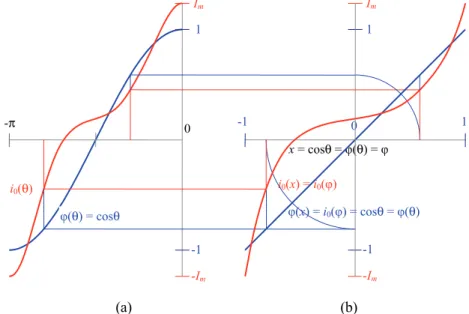
Then the mapping i0(cosθ) = i0(θ) represents the dynamic hysteresis loop branch

function i0(φ) of the magnetic flux domain variable: i0(φ)∈C[–1,1], i0(φ)∈[–Im, Im].

The functions i0(θ) and φ(θ) satisfying conditions of the Theorem I are shown in

Fig. 1.

(a) (b)

Fig. 1 – (a) Waveforms of excitation current and magnetic flux satisfying the Theorem I conditions; (b) Process of excitation

current mapping into hysteresis loop branch.

Note 1: Notation i0(θ)∈C[–π,0] means that the function i0(θ) belongs to the class

of continuous functions on the segment θ∈[–π,0] and i0(φ) belongs to the class

of continuous functions on the segment φ∈[–1,1].

x = cosθ = φ(θ) = φ i0(x) = i0(φ)

φ(x) = i0(φ) = cosθ = φ(θ) i0(θ)

φ(θ) = cosθ

-π

0 -1 1

-1 -1

-Im

-Im

Im Im

1 1

Note 2: Not losing in generality, the function φ∈[–1,1] is normalized so the proof for the case of arbitrary amplitude values φ∈[–Φm, Φm] is given in the corollary bellow.

Proof

The considered function i0(θ)∈C[–π,0], which meets the conditions (6) and

(7), belongs to the general class of periodic functions i0(2πft)∈C[2πft,

2πft+T] = 0 2

C_π. The sinusoidal magnetic flux belongs to this class as well:

φ(2πft)∈C[2πft, 2πft+T] = C₂0π. The extreme values of the same sign of these

two functions are simultaneous in time t+kT/2, k∈N, which is the reason that these two functions can be treated in the class of the functions i0(θ), φ(θ)∈

C[–π,π] whose extreme values of the same sign are simultaneous for the next variable θ values: {–π,0,π}. Let select these values as

(

)

( )

( )

0 m, 0 0 m, 0 m, i −π = −I i =I i π = −I

and

(

)

1,

( )

0 1,

( )

1,

ϕ −π = − ϕ = ϕ π = −

in such way that compliance with the conditions (6) and (8) is ensured. Then, based on the assumption that φ(θ)∈C[–π,π] is a sinusoidal function, it follows that φ(θ) = cosθ.

The functions i0(θ) and φ(θ) are given parametrically. Since the analytical

form of the function i0(θ) is unknown, it is necessary to find a new parameter

function x(θ) so that is φ(θ-1(x)) = x(θ–1(φ)). In such way a linear dependence

φ(x) = x(φ) (Fig. 1) is established, which further allows direct derivation of the function i0(φ) starting from the new parametric form of the function i0(x) and

φ(x).

By mapping of the segment θ∈[–π,0] into the segment x∈[–1,1] using the function x = cosθ (Fig. 1), the monotonic function i0(θ)∈[–Im, Im], based on (7), is

uniquely transformed into a new monotonic function

(

)

( )

[

]

0 cos 0 m, m ,

i θ =i x ∈ −I I (9)

so that holds

( )

(

)

( )

( )

(

)

( )

0 1 0 1 0 1 0 2 0 2 0 2

1 2 1 1 2 2

cos cos ,

0, 1 cos cos 1.

i i i x i i i x

x x

θ = θ = < θ = θ =

−π ≤ θ < θ ≤ ≤ θ = < θ = ≤ (10)

Also, the mapping of the segment θ∈[–π,0] into the segment x∈[–1,1] using the function x = cosθ (Fig. 1), the cosine magnetic flux function

φ(θ) = cosθ∈[–1,1] is transformed into a linear function φ(x) = cos(arccosx) = x. This function actually is the Chebyshev polynomial of the first kind T1(x) = x,

( )

( )

( )

[

]

[

]

1 _{x x , x 1,1 , 1,1 .}

−

ϕ = ϕ = ϕ ϕ ∈ − ϕ∈ − (11)

Based on equations (10) and (11) it follows that

( )

(

)

( )

( )

0 0 0 0

1 2 1 1 1 2 2 2

cos ,

0, 1 cos cos 1

i i i x i

x x

θ = θ = = ϕ

−π ≤ θ < θ ≤ ≤ θ = = ϕ < θ = = ϕ ≤ which statement was to be proved. ■

The steps in proving the theorem and the result of the theorem are graphically shown in Fig. 1.

When the extreme values of the magnetic flux function deviate from the unit values, but meet the condition

( )

( )

(

)

( )

( )

( )

0 0

0 0

min max Φ ,

max max Φ 0 ,

m

m

−π≤θ≤ −π≤θ≤

−π≤θ≤ −π≤θ≤

ϕ θ = − ϕ θ = − = ϕ −π

ϕ θ = ϕ θ = = ϕ (12)

the following corollary reformulates the Theorem I:

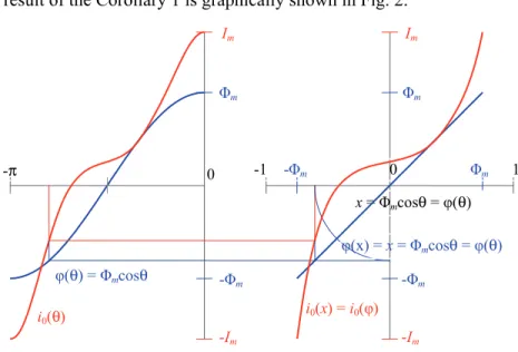
Corollary I

If the condition (8) of the Theorem I is replaced with the condition (12), then the mapping i0(Φmcosθ) = i0(θ) represents the dynamic hysteresis loop

branch function i0(φ) of the magnetic flux variable: i0(φ)∈C[–Φm, Φm], i0(φ)∈

[–Im, Im].

Note 3: Notation i0(φ)∈C[–Φm, Φm] means that the function i0(φ) belongs to the

class of continuous functions on the closed variable interval φ∈[–Φm, Φm].

Proof

When the amplitude of the sinusoidal magnetic flux deviates from the unit values, the function of the magnetic flux takes the form

( )

Φ_mcos .

ϕ θ = θ (13)

The segment θ∈[–π,0] will be now uniquely mapped to the segment x∈[–Φm, Φm] by the parameter function x = φ(θ) = Φmcosθ, so the cosine function of the magnetic flux φ(θ) = Φmcosθ ∈[–Φm, Φm] will be transformed into a linear function φ(x) = Φmcos(arcos(x/Φm)) = ΦmT1(x/Φm) = x, and its inverse function takes the form

( )

( )

( )

[

]

[

]

1 _, Φ _,Φ _, Φ _,Φ _.

m m m m

x x x

−

ϕ = ϕ = ϕ ϕ ∈ − ϕ∈ − (14)

Based on (8) and (15) it follows that

( )

(

)

( )

( )

0 0 Φmcos 0 0 , 1 2 0,

i θ =i θ =i x =i ϕ − π ≤ θ < θ ≤

1 1 1 2 2 2

Φ_m Φ_mcos x Φ_mcos x Φ_m

− ≤ θ = = ϕ < θ = = ϕ ≤ ,

The result of the Corollary 1 is graphically shown in Fig. 2.

Fig. 2 – The process of excitation current mapping into hysteresis loop branch for arbitrary magnetic flux amplitude value.

Note 4: The magnetic flux in certain operating conditions, particularly during the transition process, is not a sinusoidal function of time. The Theorem I does not apply in such cases, neither the Corollary I.

5 Discussion

1. The Theorem I, along with its Corollary I, shows that the excitation winding current characterizes qualitatively in the same way the behavior of a magnetic circuit under sinusoidal magnetic flux just as its hysteresis loop branch does.

2. The Theorem I and its Corollary I do not determines the analytical dependence of the above-mentioned functions of physical processes in the magnetic circuit, but determines the conditions under which the results of approximation theory [17 – 19] can be precisely applied. In particular, this means the following:

The mapping of the segment [–π,0] on [–1,1] by using the parametric function x = cosθ (θ = 2πt/T) the functions cos(kθ), k = 0,…,n defined on the segment [–π,0] are transformed into the Chebyshev polynomials of the first kind

T1(x) = cos(k(arccosx)), k = 0,…,n, on the segment [–1,1], which is why the

excitation current cosine polynomial is of the form

-Im

-Im

Im Im

-π ₀ -1 0 1

Φm Φm

-Φm -Φm

Φm -Φm

φ(θ) = Φmcosθ

x = Φmcosθ = φ(θ)

φ(x) = x = Φmcosθ = φ(θ)

( )

0

0

2

cos , 0, , ,

n k k

i C k k n t

T

=

π

θ =



⋅ θ = … θ = (15)

where i0(θ) meets the requirements of the Theorem I. Then this function is

directly transformed into an algebraic polynomial of the form

( )

( )

[

]

0

0

, 0, , 1,1.

n k k k

i x C T x k n x

=

=



= … ∈ − (16)

In the case of using the parametric function Φmcosθ for the mapping of [–π,0] on φ∈[–Φm, Φm], the cosine polynomial (15) is directly transformed into the algebraic polynomial of the form

( )

[

]

[

]

0

0

, 0, ,

Φ

Φ 1,1 , Φ ,Φ ,

n k k

k m

m m m

i C T k n

x =

ϕ

ϕ = = …

ϕ = ∈ − ∈ −

     

ϕ



₍₁₇₎

with identical values of the coefficients Ck as in (15), (16) and (17).

This is the main result in the practical application of the Theorem I and its Corollary I (in further text Theorem I) regarding the computing efficiency and approximation accuracy.

5.1 Technical requirements for obtaining Chebyshev nodes and

determination of the subsets of samples that represent the nodes of the first and the second kind.

Technical requirements for the successful application of the Theorem I imply the use of the zero crossing sampling system, such as the set of two Agilent 3458 A multimeters that was used in the experimental validation of the Theorem I together with the sinusoidal voltage source Fluke 6100 A with

f= 50 Hz mains frequency. A single phase transformer 220 V/57.73 V,

Sn = 100 VA was used as a measuring object for this purpose.

The sampling rate of 10 kHz gives a set of 101 synchronized excitation current and magnetic flux samples across the electric angle segment θ∈[–π,0], (θ = 2πft). The first sample from this set that corresponds to the negative extremum, for both the flux and the excitation current, is indexed with the index value 0. Then, the last sample from this set that corresponds to the positive extremum for both the flux and the excitation current is indexed with the index value 100.

Let the sample index be denoted with k. Then the CHN_I nodes are determined by the expression [18]

(

)

(

)

2 2 1

cos , 1, 2, , 0 ,

2

10 ,

2

ChI

kChI ChI

ChI

n k T

x k n

n <

− + π ω

and the CHN_II nodes are determined by the expression [18]

(

)

cos , 0, , 1 100 ,

1 1 , 2 .

kChII ChII

ChII

k T

x k n

n

π ω

= = … − ≤ π =

− (19)

For obtaining the series of ascending sample values for the electric angle segment θ∈[–π,0], the expressions (18) and (19) are to be rearranged into the appropriate form

(

)

(

)

2 2 1

cos , 1, 2, , ,

2

ChI

kChI ChI

ChI

n k

x k n

n

− + π

= _− _ = …

  (20)

and

(

)

cos , 0,1, , 1 .

1

kChII ChI

ChII

k

x k n

n

π

= −π = … −

−

 

 

  (21)

Finally, by means of the substitution Δθ = π/100, where Δθ represents the sampling step, expressions (20) and (21) get the form

(

)

(

)

2 2 1 100

cos , 1, 2, , ,

2

ChI

kChI ChI

ChI

n k

x k n

n

− + Δθ

= _− ⋅ _ = …

  (22)

and

(

)

100

cos , 0,1, , 1 .

1

kChII ChII

ChII

k

x k n

n

⋅ Δθ

= − π = −

− …

 

 

  (23)

Based on (22), the expression for determining index values of the CHN_I nodes is derived

(

)

(

)

2 2 1 100

100 , 1, 2, ,

2 .

ChI

ChI ChI

ChI

n k

k k n

n

− +

= − = … (24)

The above expression allows only those values for nChI that produce the integer values for kChI. Therefore, nChI can take only the values from the set {50,25,10,5,2,1}.

Similarly, from (23) it is obtained

(

1

)

1 100

, 0,1, , ,

ChII ChII

ChII

k

k k n

n

⋅

= = … −

− (25)

and integer values for kChII will be obtained only if nChII takes values from the set {101,51,26,11,6,5,3,2}.

from the Table 1. In the case of nChII = 101, the entire set of samples would be included and thus an analysis of the error distribution could not be possible.

Table 1

Identification of the sample subsets that represent Chebyshev nodes.

for Index of the sample that coincides with a node index

nChI = 10 {5,15,25,35,45,55,65,75,85,95}

nChII=11 {0,10,20,30,40,50,60,70,80,90,100}

nChII=21 {0,5,10,15,20,25,30,35,40,45,50,55,60,65,70,75,80,85,90,95,100}

nChI=50

{1,3,5,7,9,11,13,15,17,19,21,23,25,27,29,31,33,35,37,39,41,43,45,47,49,51, 53,55,57,59,61,63,65,67,69,71,73,75,77,79,81,83,85,87,89,91,93,95,97,99}

nChII=51

{0,2,4,6,8,10,12,14,16,18,20,22,24,26,28,30,32,34,36,38,40,42,44,46,48,50, 52,54,56,58,60,62,64,66,68,70,72,74,76,78,80,82,84,86,88,90,92,94,96,98,100}

5.2 The discrete orthogonality of the Chebyshev polynomials and two examples of practical application of the Theorem I

An interpolation polynomial over n+1 CHN_I nodes from normalized flux domain segment x∈[–1,1] has the following form [18]

( )

( )

( )

( )

[

]

0 0 0

0 1

1

, 1,1 .

2

n n

k k k k

k k

i x c T x c T x c T x x

= =

=



′

= +



∈ − (26)

By virtue of the discrete orthogonality [17, 18] of the Chebyshev polynomials over CHN_I nodes, the ck coefficients are computed by two equivalent expressions

( )

( )

(

(

)

)

(

)

(

)

(

)

1 0 1

2 1 2 1 2

, cos

1 2 1

0, , , 1 ,

n

k j k j j

j

ChI

n j c i x T x x

n n

k n n n

+

=

= + − + π

= ⋅ − + + = … + =      



(27) and

(

)

(

)

(

)

(

)

(

)

(

)

(

)

(

)

1 0 1

2 1 2 1 2

cos ,

1 2 1

0, , , 1

2 1 2 1

2 1 . n k j ChI n j

c i k

n n

k n n n

n j

n

+

=

+ − + π

= ⋅ −

+ +

= … + =

 + − + π  

−

  _{ }

 ₊  _{ }

 



₍₂₈₎

( )

[

]

0 0

0 1

1

cos cos , ,0 .

2

n n

k k

k k

i c k c c k

= =

θ =



′

θ = +



θ θ∈ −π (29)

An example of the Theorem I application by means of (26) – (29) is represented for the set of nchI = 10 Chebyshev nodes of the first kind in tabulated form in Table 1 and in graphical form in Fig. 3.

Similarly, n+1 Chebyshev nodes of the second kind have the following expressions [18]:

( )

( )

( )

1

( )

( )

[

]

0 0 0

0 1

1 1

, 1,1 ,

2 2

n n

k k k k n n

k k

i x c T x c T x c T x c T x x

−

= =

′′

=



= +



+ ∈ − (30)

( ) ( )

(

)

(

)

0 0 2 , cos

0, , , 1 ,

n

k j k j j

j

ChII j

c i x T x x

n n

k n n n

=

π

 

′′

= = _ − π_

  = … + =



(31)

(

)

(

)

0 0 cos ,

0, , , 1

2

.

k ChII n j j j

c i k

n n

k n n n

n

=

π π

   

′′

= _ − π_{ } − π_

   

= … + =



(32)

( )

1

[

]

0 0

0 1

1 1

cos , ,0 ,

2 cos 2 cos

n n

k k n

k k

i c k c c k c n

−

= =

′′

θ =



⋅ θ = +



θ + θ θ∈ −π (33)

An example of the Theorem I application by means of (30) – (33) is given for the set of nchII = 11 Chebyshev nodes of the second kind in tabulated form in Table 3 and in graphical form in Fig. 4.

Table 2

Cebyshev nodes of the first kind and the coefficients of interpolation polynomial for Chebyshev polynomials basis and for monomials basis.

nChI

node index

sample φ (index)

[Wb]

sample φ (index) normalized

sample i0

(index) [A] coefficients for Chebyshev polynomial basis coefficients for monomial xk

basis

5 -0.0013432231 -0.987688341 -0.117733834 c0 0.0276080973 a0 0.019275485

15 -0.0012144271 -0.891006524 -0.071737436 c1 0.0897163468 a1 0.015673906

25 -0.0009661704 -0.707106781 -0.020843621 c2 -0.0095927426 a2 0.000158380

35 -0.0006214148 -0.453990499 0.006715073 c3 0.0301421501 a3 0.057566282

45 -0.0002143542 -0.156434465 0.016626753 c4 -0.0048764490 a4 0.045836512

55 0.0002143542 0.156434465 0.021983351 c5 0.0037755316 a5 0.065155372

65 0.0006214148 0.453990499 0.033870687 c6 -0.0003212031 a6 -0.121367066

75 0.0009661704 0.707106781 0.059072496 c7 0.0005555446 a7 -0.053735629

85 0.0012144271 0.891006524 0.090991235 c8 0.0004339397 a8 0.055544283

Table 3

Cebyshev nodes of the second kind and the coefficients of interpolation polynomial for Chebyshev polynomials basis and for monomials basis.

nChII

node index

sample φ (index) [Wb]

sample φ (index) normalized

sample i0

(index) [A]

coefficients for Chebyshev polynomial basis

coefficients for monomial xk basis

0 -0.0013594619 -1.0000000000 -0.123795498 c0 0.0276971868 a0 0.019154967

10 -0.001294644 -0.9510565163 -0.098412061 c1 0.0896541475 a1 0.014298962

20 -0.0011041222 -0.8090169944 -0.044543009 c2 -0.0095414213 a2 0.002200856

30 -0.0008038880 -0.5877852523 -0.003735111 c3 0.0300749038 a3 0.075706177

40 -0.0004232631 -0.3090169944 0.013030176 c4 -0.0047526785 a4 0.048223005

50 0.0000000000 0.0000000000 0.019154967 c5 0.0036494057 a5 -0.003897475

60 0.0004232631 0.3090169944 0.026337257 c6 -0.0000148624 a6 -0.147501281

70 0.0008038879 0.5877852523 0.045335193 c7 0.0004456793 a7 0.045019320

80 0.0011041222 0.8090169944 0.074312542 c8 0.0004815688 a8 0.088776878

90 0.0012946439 0.9510565163 0.107005978 c9 -0.0000286386 a9 -0.007331486

100 0.0013594619 1.0000000000 0.123795498 c10 -0.0000424001 a1 -0.010854426

(a) (b)

Fig. 3 – (a) Graph of the cosine interpolation polynomial i0(θ) over 10 CHN_I nodes

in the electrical angle domainθ∈[–π,0]; (b) Graph of the algebraic interpolation polynomial i0(x) over 10 CHN_I nodes in normalized flux domain x∈[–1,1].

5.3 Metrological aspects of the Theorem I

Besides the modeling of the dynamic hysteresis loop branches for different purposes, the Theorem I has practical metrology application in determining three parameters of the given magnetic circuit:

1. Coercive current (field),

2. Area of the closed hysteresis loop and 3. Remanence (redsidual) flux.

φ(θ)

i0(θ)

-π

1

0

-1

-1 1

1

-1

i0(φ)

Im Im

(a) (b)

Fig. 4 – (a) Graph of the cosine interpolation polynomial i0(θ) over 11 CHN_II nodes in

the electrical angle domainθ∈[–π,0]. (b) Graph of the algebraic interpolation polynomial i0(x) over 11 CHN_II nodes in normalized flux domain x∈[–1,1].

This is the main reason why the theorem was experimentally validated on a single phase transformer as a measuring object, in order to be applicable without limitation to either the Epstein frame (single sheet or toroidal core specimen), in which case the H(B) interpolation polynomial is to be determined [25, 26], or the arbitrary transformer magnetic circuit where the interpolation polynomial i0(φ) is to be determined.

1. The coercive current (field) determination

In the Fig. 5 is represented the closed dynamic hysteresis loop that consists of the interpolation polynomial pnCh(0) for ascending loop branch and –pnCh(–x), the centrally symmetric to the origin i0-φ polynomial, for descending loop

branch. The polynomial ( )

Ch n

p x has the form of (26) for CHN_I nodes, or (30) for CHN_II nodes [18].

The coercive current is then directly calculated based on

( )

( )

0 0 nCh 0 .

i = p (34)

By means of the substitution x = 0 in (26) for CHN_I nodes, one can get the simple expression (35)

( )

( )

[ ]

( )

0 1 0 2

1

2

1

0 0 1 ,

2 ChI

i

n n i

i

n

i p_{= −} c c

=

= = +



− (35)

Im

1

0

-1

φ(θ)

i0(θ)

-π -1 1

1

-1

i0(φ)

Im

(a) (b)

Fig. 5 – (a) DHLB’s represented by the interpolation polynomials (16) on the domain segmentx∈[–1,1]; (b) DHLB’s represented by the interpolation

polynomials (17) on the domain segmentφ∈[–Φm, Φm].

and in particular for n = 9

( )

( )

0 1 0 2 4 6 8

1

0 0 .

2

ChI n n

i = p_{= −} = c −c +c −c +c (36)

Similarly, based on (30) for CHN_II it holds

( )

( )

( )

( )

1 2

2

0 1 0 2

1 2

1 1

0 0 1 1 ,

2 2

ChI

n

n i

n n i n

i

i p c c c

−

 

 

   

   

= −  

 

= _{ }

= = +



− + − (35)

and in particular for n = 10

( )

( )

0 1 0 2 4 6 8 10

1 1

0 0

2 2 .

ChI n n

i = p _{= −} = c −c +c −c +c − c (36)

2. The area of the closed hysteresis loop calculation

When determining the coercive current, it does not matter if the polynomial form of (16) or (17) is used. That is illustrated in Fig. 5. But it is not so obvious for the calculation of an arbitrary closed hysteresis loop area. Namely, it seems that this calculation requires the use of the interpolation polynomial form (17):

( )

(

)

(

)

Φ

Φ

d .

m

Ch Ch

m

H n n

S p p

ϕ

−

=



ϕ + −ϕ ϕ (37)

pnCh(x) Im

-Im -Im

-1 1

Im

-1 1 -Φm Φm

i0(0) i0(0)

-pnCh(-x)

pnCh(φ)

-pnCh(-φ) -pnCh(-x)

Integration gives as a result for CHN_I nodes [ ]

(

)(

)

0 2 1 2

4Φ ,

2 2 1 2 1

i H m i n c c S i i ϕ = = − − +    





 (38)

and in particular for n = 9

0 2 4 6 8

4Φ .

2 1 3 3 5 5 7 7 9

H m

c c c c c S

ϕ = − + + +

⋅ ⋅ ⋅ ⋅

  

 

 _{ }

  (39)

Similarly, the result for CHN_II nodes is

( ) [ ]

(

)(

)

[ ]

[

]

(

)

(

[

]

)

0 2 1 1 2 2

4Φ ,

2 2 1 2 1 2 2 2 1 2 2 1

i H m i n n c c c S

i i n n

ϕ = − = − − − + − +    





 (40)

and in particular for n = 10

0 2 4 6 8 1 10

4Φ

2 1 3 3 5 5 7 7 9 2 9 11 .

H m

c c c c c c S

ϕ = − + + + − ⋅

⋅ ⋅ ⋅ ⋅ ⋅

   

 

 _{ } 

  (41)

The expressions (38) and (40) point out the important fact regarding numerical calculations, that an area of the closed hysteresis loop can be calculated directly on the basis of ck coefficients and the Φm value without the need of generating an

interpolation polynomial. The same holds for the determination of the coercive current.

3. The remanence flux determination

Since the polynomial pnCh(x) (16) has only one real zero, the iterative procedure

( )

( )

1 , Ch Ch n k k k n k p x x x p x + = −

′ (42)

gives the value of the normalized remanence flux xr, and by virtue of xr is obtained the actual value of the remanence flux φr

Φ .

r =xr m

ϕ (43)

5.4 Convergence of an interpolation polynomial to the experimentally obtained DHLB curve and analysis of the error distribution

The measure of approximation accuracy in the case of representing DHLB by using an interpolation polynomial of the form (26) and (30) can be observed by the corresponding error distribution functions

( )

0

( )

( )

, 0,...,100,

ChI ChI

n i i n i

e x =i x − p x i= (44)

and

( )

0

( )

( )

, 0,...,100.

ChII ChII

n i i n i

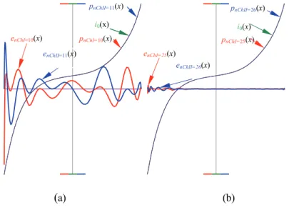
(a) (b)

Fig. 6 – (a) DHLB and pnChI ordinate values are magnified by 10 times, whereas

enChI ordinate values are magnified by 200 times for nChI = 10;

(b) The same holds for DHLB, pnChII and enChII ordinate values for nChII = 11.

(a) (b)

Fig. 7 – (a) DHLB, pnChI for nChI = 10 and pnChII for nChII = 11 ordinate

values are magnified by 10 times, whereas enChI for nChI = 10

and enChII. for nChII = 11 are magnified by 1000 times;

(b) The same holds for DHLB, pnChI, pnChII, enChI

and enChII for nChI = 25 and nChII = 26.

The graphics of the experimentally obtained DHLB curve are represented in Fig. 6, as well as the interpolation polynomials pnChI(x) and pnChII(x) for

enChI=25(x)

i0(x)

pnChII=26(x)

pnChI=25(x)

enChII=26(x)

enChI=10(x)

enChII=11(x)

pnChII=11(x) i0(x)

pnChI=10(x)

-1 1

-1 1

1

-1

1

-1

i0(x)

pnChI(x)

enChI(x) enChII(x)

-Im -Im

Im Im

i0(x)

nChI = 10 and nChII = 11, and error distribution functions enChI(x) and enChII(x). The ordinate values of the DHLB curve and pnChI(x) and pnChII(x) polynomials are magnified by 10 times, whereas the ordinate values of the error distribution functions enChI(x) and enChII(x) are magnified by 200 times.

Apart from the approximation accuracy of an interpolation polynomial, an error distribution function enables the observation of the relationship between the degree of an interpolation polynomial and its convergence to the approximated DHLB. As an illustration of convergence behavior, Fig. 7 represents the graphics of the experimentally obtained DHLB curve and its interpolation polynomials for nChI = 10, nChII = 11, nChI = 25 and nChII = 26 nodes, together with the corresponding error distribution functions. As a result of a very good convergence of the higher degree interpolation polynomial to the DHLB, the magnification of the polynomial ordinate values is retained at 10 times, whereas the ordinate values of the error distribution functions are magnified by 1000 times.

6 Conclusion

An excitation current that fulfils the conditions given in the Theorem I can be accurately approximated by using the cosine polynomial of the form (15), whereas its corresponding DHLB can be approximated by using the corresponding algebraic polynomial of the form (16) i.e. (17), with an equivalent accuracy of approximation for the either normalized or arbitrary magnetic flux amplitude values. From the point of view of metrology, it is important that the above mentioned polynomial can be generated over the discrete subsets of the measured samples, and that an approximation error can be effectively affected by the sampling frequency and the sampling resolution.

The proposed method enables us to express explicitly the DHLB by cosine polynomial in the time (electric angle) domain and by algebraic polynomial in the magnetic flux domain. The earlier represented method of analyzing the hysteresis loops by using the Fourier analysis (Masheva, Geshev and Mikhov [27]) gives an explicit expression of a hysteresis loop branch only for the electric angle domain in the form of a trigonometric polynomial. Actually, the Theorem I defines the conditions for using both of the above mentioned methods. Therefore, a detailed comparative analysis of the approximation efficiency in the dependence of using these two methods over CHN_I and CHN_II nodes should be the subject of the future work.

Chebyshev nodes can be used with no constraints by virtue of the producer catalogues.

7 References

[1] J. A. Ewing: Experimental Researches in Magnetism, Proceedings of the Royal Society of London, Vol. 38, 1884 – 1885, pp. 58 – 62.

[2] E. Madelung: Uber Magnetisierung durch schnellverlaufende Strome und die Wirkungweise der Rutherford-Markoni Magnetodetektors, Annaler der Physik, Vol. 322, No. 10, 1905, pp.861 – 890.

[3] M. P. Langevin: Magnetisme et theorie des electrons, Annales de Chimie et de Physique Vol. 5, 1905, pp. 70 –127.

[4] M.L. Brillouin: Les moments de rotation et le magnetisme dans la mechanique ondulatoire, Journal de Physique et Le Radium, Vol. 8, No. 2, 1927, pp. 74 – 84.

[5] F. Preisach: Uber die magnetishe nachwirkung, Zeitschrift für Physik, Vol. 94, 1935, pp. 277 – 302.

[6] D. C. Jiles, D. L. Atherton: Theory of ferromagnetic hysteresis, Journal of Magnetism and magnetic materials, Vol. 61, 1986, pp. 48 – 60.

[7] J. Fisher, H. Moser: Die nachbildung von magnetisierungscurven durch einfache algebraishe oder transzendente funktionen, Archiv fur Electrotechnik, XLII, No. 5, 1956, pp. 286 –299. [8] C.F. Trutt, E. A. Erdelyi, R.E. Hopkins: Representation of the Magnetization Characteristic

of DC Machines for Computer Use. IEEE Transactions on Power Apparatus and Systems, Vol. PAS–87, No.3, 1968, pp. 665 – 669.

[9] G.F.T. Widger: Representation of Magnetisation Curves Over Extensive Range by Rational Fraction Approximations, Proceedings of IEE, Vol. 116, No.1, January 1969, pp. 156 – 160. [10] J.R. Brauer: Simple Equations for the Magnetization and Reluctivity Curves of Steel, IEEE

Transactions on Magnetics, Vol. 11, No. l, 1975, pp. 81.

[11] J. Rivas, J.M. Zamarro, E. Martin, C. Pereira: Simple Approximation for Magnetization Curves and Hysteresis Loops, IEEE Transactions on Magnetics, Vol. 17, No. 4, 1981, pp.1498 – 1502.

[12] I. D. Mayergoyz: Mathematical Models of Hysteresis and Their Applications, Elsevier Science, Amsterdam, 2003.

[13] G. Bertotti, Hysteresis in Magnetism, Academic Press, San Diego, USA 1998.

[14] A. lvanyi: Hysteresis Models in Electromagnetic Computation, Akademiai Kiado, Budapest, 1997.

[15] E. Della Torre: Magnetic Hysteresis, IEEE Press, New York, USA, 1999.

[16] J. Takacs: Mathematics of Hysteretic Phenomena, Hoboken Wiley/VCH, New York, USA, 2003.

[17] G.M. Phillips: Interpolation and Approximation by Polynomials, Springer–Verlag, New York, USA, 2003.

[18] J.C. Mason, D.C. Handscomb, Chebyshev Polynomials, CRC Press, Washington, D.C, USA, 2003.

[19] D. Jackson: The Theory of Approximation, Chapter IV: Trigonometric Interpolation, pp. 109-148, American Mathematical Society Colloquium Publications, Vol. XI, 1930.

[21] J.Krstović, R.Radosavljević: Design of distribution transformers, Akademska misao, Belgrade, 2009. (In Serbian).

[22] IEC 60404-2: Methods of measurement of the magnetic properties of electrical steel sheet and strip by means of an Epstein frame IEC Standard Publication, Geneva: IEC Central Office, Switzerland, 1996.

[23] ASTM: A343/A343M-03 Standard Test Method for Alternating-Current Magnetic Properties of Materials at Power Frequencies Using Wattmeter-Ammeter-Voltmeter Method and 25-cm Epstein Test Frame, 2008.

[24] ASTM: A927/A927M-04 Standard Test Method for Alternating-Current Magnetic Properties of Toroidal Core Specimens Using the Voltmeter– Ammeter-Wattmeter Method, 2004.

[25] F. Fiorillo: Measurements of Magnetic Materials, Metrologia, Vol. 47, 2010, S114 – S142. [26] S. Tumanski: Handbook of Magnetic Measurements, CRC Press, Boca Raton, FL, USA,

2011.