FUNDAÇAo
GETUUO VARGAS
EPGE
Escol. de P6s-Graduaçãoem Economia
Ensaios Econômicos
Escola de
セセMMMMMMMM MMMMMMMM
Pós Graduação
em Economia
da Fundação
Getulio Vargas
AI"
532
ISSN 0104-8910
Regional or educational disparities? A counterfactual exercise
Angelo José Mont'Alverne
Pedro Cavalcanti Ferreira
Márcio Antônio Salvato
Regional or Educational Disparities?
A Counterfactual Exercise*
Angelo José Mont'Alverne Duarte
t
Pedro Cavalc anti Ferreira
jMárcio Antônio Salvato§
December 2, 2003
Abstract
This work investigates the impact of schooling Oil income distribution in
statesjregions of Brazil. Using a semi-parametric model, discussed in
Di-Nardo, Fortin & Lemieux (1996), we measure how much income diíferences
between the Northeast and Southeast regions- the country's poorest and rich-est - and between the states of Ceará and São Paulo in those regions - can be
explained by differences in schooling leveIs of the resident population. U sing
data from the National Household Survey (PNAD), we construct
counterfac-tual densities by reweighting the distribution of the poorest region/state by
the schooling profile of the richest. We conclude that: (i) more than 50% of the income di:fference is explained by the di:fference in schooling; (ii) the high-est deciles of the income distribution gain more from an increase in schooling, closely approaching the wage distribution of the richest region/state; and (iii) an increase in schooling, holding the wage structure constant, aggravates the wage disparity in the poorest regions/ states.
JEL Classification Codes: C14; 120 e J31.
*We gratefully acknowledge the comments and suggestions of Luiz Henrique Braido, Luiz Re-nato Lilna, Carlos Eugênio da Costa, Samuel Pessôa, Marcelo Fernandes, ReRe-nato Flôres and the participants in a seminar at EPGE/FGV. All remaining errors are ours. We thank CNPq, Banco Central do Brasil and PUC.Minas for financiaI support.
tEPGE/FGV and Banco Central do Brasil, e-mail: [email protected] tEPGE/FGV, e-mail: [email protected]
1
Introduction
Disparities in income between regions of Brazil, notably between the Southeast and the North and Northeast, have been a longstanding subject for debate among acad-emics, policymakers and members of the political class. As far back as the mid-19th century, Emperor Dom Pedro II remarked that he would seU his crown to feed the hungry northeasterners. Over this century and a half, many diagnoses have been conducted and programs implemented trying to diminish this inequality. Govern-ment policies intensified and became systematic starting in the 19SOS. Following the lead of the economist Celso Furtado, the document "Uma Política para o De-senvolvimento do Nordeste" (" A Policy to Develop the Northeast" ) was published, which suggested industrialization as a way to reduce income disparities between the Northeast and Southeast . This document inspired the creation of two agencies -SUDENE (Northeast Development Superintendency) and SUDAM (Amazon Devel-opment Superintendency) - along with two regional develDevel-opment banks, the BNB and BASA. The 1988 Federal Constitution chipped in by determining that of 3% of revenues from taxes on income and manufactured products must be allocated to programs to finance the productive sector in the North, Northeast and Midwest reglOns.
Despite the large number of governmental organs and programs at the federal and state leveIs devoted to regional economic development, government policies implemented over the past 50 years have mainly focused on the same instruments: tax incentives and public credits to subsidize private initiative, along with direct government spending on infrastructure projects. It is estimated that between 1989 and 2002, the constitutional funds for regional development spent some US$ 10 billion. Although successful in some respects, such as accelerating industrialization of the N ortheast and N orth, these policies have not managed to transform social indicators by reducing the rate of poverty and changing the distribution of income in these regions.
In the past decade, a new approach has emerged to the problem of regional inequality in Brazil. It is based on the thesis that low per capita income in the North and Northeast regions is related to the concentration of individuaIs with low schooling leveIs (human capital) and low physical capital, which together limit their ability to earn. In this form, reducing regional inequality cannot be divorced from combating poverty, so what is needed is a policy stressing education and professional training and programs for access to credito
Pessoa (2000) suggests there are two facets to the problem of unequal income : the first and most important involves the difference in per capita income between the regions; and the second, less significant, refers to the spatial distribution of production. According to the author, supposing perfect labor mobility between the regions, there can only be an income differential between them if the characteristics of the individuaIs in the regions differs. In this way, the development policies based on subsidies and accumulation of physical capital adopted in Brazil have always tried to focus on the first problem but in reality are more suited to addressing the second facet . Barros (1993), Barros and Mendonça (1995) and Barros, Camargo and Mendonça (1997) strengthen the thesis of the importance individuaIs' charac-teristics, particularly of education leveI, in determining income differences, based on empirical evidence .
by an income distribution parameter, were equal to that of another country. The authors conclude that inequalities in human capital qualifications and transfers ex-plain nearly 2/3 of the difference in inequality leveIs between Brazil and the United States.
In this work we analyze the effects of an alteration in the educational charac-teristics of a region1 on its wage distribution. We use a non-parametric approach presented in the work of DiNardo, Fortin and Lemieux (1996), in which they an-alyzed the effects of institutional and labor-market factors, such as the minimum wage leveI and degree of unionization, on wage distribution in the United States. In this methodology, the effects on wages of a determined characteristic of the population or factor that influences its behavior are measured by applying a non-parametric method of estimating the density function, and reweighting the samples by the characteristic/factor of interest. This leads to constructing what is called a counterfactual distribution, which can be compared with the original wage dis-tribution of the population. In our case, we work with the disdis-tribution of income from labor (referred to simply as income for economy), since we have no data on minimum wages for Brazil. 2
This approach has the same foundation as the decomposition of Oaxaca (1973)3, which is based on the construction of counterfactuals, but unlike the original idea - which worked only with the means of the distributions - we analyze the entire distribution. The methodology we employ allows us to visualize the income density function clearly and to see the changes that would occur in this distribution if there were any changes in the population's educational conditions, maintaining the original income distribution structure in place. In this sense, instead of focusing the study of income and educational differential on some index of inequality, such as the coefficients of Gini and of Theil, or the variance of the logarithm of income, we intend to derive our conclusions by observing the entire income distribution, using measures of distribution differences and the Komogorov-Smirnov distribution inequality testo
Construction of the counterfactual distributions is done by reweighting the sam-pIe according to some characteristic of interest. In other words, to study, as in our case, the effects of schooling leveI on income, we estimate the income distribution by reweighting the samples available in such a way that they become part of the profile of a population with the desired schooling profile. In this form, we can obtain what the income distribution of a region would be if it had the schooling characteristics of another region, maintaining its original income structure. It should be clear that there is a limitation to this methodology, since it only considers partial effects and cannot analyze the effects in general equilibrium. Nevertheless, this approach will be quite useful to answer questions of the type: What would be the income distri-bution in the state of Ceará if its education conditions were similar to those of the
1 By region we mean a determined geographic area, which can be a municipality, state, set of states, geographic region or a country, about whose inhabitants we want to study a certain characteristic.
2In Brazil, worker pay is rarely computed in terms of an hourly wage, but rather in relation to a monthly salary. The government establishes the minimum salary (nowadays adjusted yearly) for full-time employees, and most job earnings, as well as social security benefits, are set in mul-tiples of this minimum. 80, although speaking of a minimum wage for Brazil is in the strictest sense a misnomer, the expression minimum wage can be employed without causing any distortion. However, based on the characteristics measured in our database, as indicated, we generally speak of income, meaning job income, and in some instances use minimum salary when the situation specifically warrants it.
state of São Paulo?
To answer that question, for example, we measure the change in the income distribution in Ceará and the Northeast Region if the resident population in these regions had the same schooling as those in São Paulo and the Southeast Region.4
In the following section we present some facts that illustrate the problem of in-equality in Brazil. In Section 3 we present the data used in our analysis. In Section 4 we discuss in some detail the methodology for arriving at the weighted kernel density estimators and constructing the counterfactual densities, besides present-ing some parametric and non-parametric measures used to compare the estimated densities. The results are presented in Section 5,and we conclude in Section 6.
2
Stylized Facts
The inequality among Brazilian regions and states can be seen both from indica-tors of the well-being of the population and their leveI of income. The difference between the Human Development Indices (HDI) in the regions of interest went down belween 1991 and 2000. The dislance belween HDIs in lhe Norlheasl and Soulheasl, for example, which was 0.16 in 1991, decreased lo 0.12 in 2000 (Table 1) 5. Nevertheless, the relative positions of the regions have not changed since the indices were computed for the first time in 1970. Besides this, the relative position of the states also did not change much in the same period, inasmuch as the nine Northeastern states remained among the 11 units of the federation6 with the worst
HDIs throughout the interval 1971-1990. The disparity in income, measured by the coefficients of Theil and Gini7, worsened in all Brazilian regions in the 1970s and 80s, and improved slightly in the 90s. This decline was more pronounced in the North and Northeast regions, making them even more unequal when compared wilh lhe Soulheasl (Table 2) .
Table 1
Human Development Index - HDI
Human Development
Year Brazil Regions
Index- HDI Midwest Northeasl North Southeast
H DI-Educalion 1991 0.745 0.778 0.606 0.705
2000 0.849 0.877 0.762 0.818
H DI-Lilespan 1991 0.668 0.682 0.587 0.637
2000 0.731 0.747 0.669 0.706
HDI-Income 1991 0.681 0.699 0.564 0.614
2000 0.723 0.747 0.614 0.640
HDI-Tolal 1991 0.698 0.720 0.586 0.652
2000 0.768 0.790 0.682 0.722
Source: Authors
4 As shall be seen in the next section, in fact we do not consider the entire Southeast Region. 5We calculated the HDIs in the regions following the methodology of the PNUD .
6The Federal District (DF) , location ofthe nation 's capital , Brasília , is counted along with the states as a unit of the federation. From here on we will simply use the term state unless specifically speaking of the DF.
7The value of both coefficients varies between O, meaning no inequality, and 1, when it is at its maximum.
0.812 0.886 0.709 0.759 0.732 0.768 0.751 0.805
Soulh
Table 2
Coefficients of Theil and Gini of Labor Income
Theil Gini
1970 1980 1991 1981 1990 2001
North 0.44 0.56 0.72 0.51 0.58 0.57
Northeast 0.57 0.65 0.78 0.57 0.63 0.60
Midwest 0.55 0.66 0.70 0.58 0.61 0.60
Southeast 0.61 0.60 0.66 0.56 0.58 0.57
South 0.53 0.58 0.63 0.54 0.58 0.55
Brazil 0.68 0.70 0.78 0.58 0.61 0.60
Source.IPEA
In terms of per capita GDP, the regional differences have remained the same
since the 19408 (Graph 1). In fact, the relative participation of the Northeast in
national GDP went down, from 16.7% in 1939 to 14.8% in 1960, and again to 13.1% in 20008
Graph 1
Per Capita Income (in log)
8 5 , - - - - , - - - - , - - - , - - - - , - - - - , - - - - , - - - - , - - - , - - - - , - - - - , - - - - , - - - - "
90 - - - T - - - "1 - - - -I - - - -1- - - - r - - -T - - - "1 - - -
Mセ L@ MBBG セセ
BBッ^|BBBBBNLiッBBG
M YP M GB LiG Mセ@
85
8 o
, ,
I I I I I I
MMM t MMMセMMMセMMMMiMMMMイMMM t MM
I I I I
MMMャMMMセMMMMiMMMMMMM
, ,
1- - - -1- - - - r - - -T - - -
-7.5 - - -
-7 o - - - _ J ____ 1 _ _ _ _ 1 _ _ _ _
, , , --*- NE
65 ___ セ@I ___ セ@I ____ :_ _ I _ __ セ@I ___ セ@I ____ : ____ :_ _ _ _ I I _ SE
VP ャZ ]]]ゥ]]
セセセセ]]
MM⦅lMMMMl⦅MM⦅ャMMMMQ⦅MM⦅ャMMMM⦅lMMMM
l⦅セ] MKMコ]]] b]r セ@
1939 1944 1949 1954 1959 19&4 1969 1974 1979 1984 1989 1994 1999
The data frem the 2000 census show that there is a positive linear relation between the per capita income in the states and the average schooling leveIs of the population older than 25 (Graph 2), which corroborates the thesis that the regional income disparities reflect the differences in human capital of the people in those reglOns.
Graph 2
Per Capita Income x Average Schooling
500
450 - - - -.{UゥG}セ@
-400
セ@
350 - - - Mセ]ct@•
E 300 o
o
..
250:§
セ@ 200
•
MMMMMMMMMMMMMMMMMMMMMMMMMMM セ@ MMMMMMM セ MMMMMMMMMMM
. . . • IRlo de Janeiro I
U
•
150..
IMinas Gerais I---
.-100
50
....
.
M セ MMMMMMMMMMMMMMMMMMMMMMMMMMMMMMMMMMMM
fPiaUil
A •
IserglPe IMMセMMMMMMMMMMMMMMMMMMMMMMMMMMMMMMMMMMMMMMMMMMMMMMM
4
Years or Schooling
3
Data
We used data from the National Household Survey (PNAD) for 1999 (conducted by the Brazilian Institute of Geography and Statistics - IBGE), with the weighting obtained from the results of the 2000 census. The results of the PNAD are presented both in terms of individuaIs and households. In the case of the individual study, which is of Qur interest, it gives information on general characteristics (current state of residence, age, sex, race, color, etc.)[Are you Bure both race and color are included?], migration characteristics (birth state, state of residence 5 years before the study, etc.), education, work and income of the subjects. We give each individ-ual a weight, which translates into how much persons with his/her characteristics represent in relation to the overall population.
The sample used consists of the individuaIs with positive income from labor in the reference month ofthe survey (September 1999), with known schooling leveI and working at least 40 hours a week. We excluded those working less than this to try to make income comparisons uniform and approximate the income measurements used here to those of wages, since this latter variable would be the ideal for this type of study (see footnote 2 above).
A total of 352,393 people were interviewed throughout the country, with 67,111 being less than 10 years old at the time, and for whom no questions were asked about labor and income. Of the 285,282 remaining people, only 173,634 were eco-nomically active9, and of these 3,265 did not state their income and/or schooling,
leaving 170,369 people. From this sample for Brazil at large, we extracted 5 sub-samples according to the state of residence: Ceará State (CE); São Paulo State (SP), Northeast Region (NE); Southeast Region, excluding the state of Espírito Santo (SEI); and Southeast Region excluding the states of Espírito Santo and São Paulo (SE2) . 10
We chose the Northeast and Southeast regions because they have the lowest and highest respective per capita incomes of the five Brazilian regions. We chose
9The economically active population is ma de up of those occupied or who are actively looking for work.
lOSE2 comprises the states of Rio de Janeiro and Minas Gerais, respectively the second and
the states of Ceará and São Paulo, in the Northeast and Southeast, respectively, because Ceará, despite being one of the poorest states in the country, is pointed out as an example of success in implementing development policies based on attracting private industrial investments, and São Paulo beca use it is the richest state in the country. We excluded Espírto Santo beca use it has a much less developed and industrialized economy than the rest of the Southeast states, to the point of its also being the target of pubic policies to fight regional inequalities (it is even included in the SUDENE area) . We also decided to consider a sub-sample without the state of São Paulo, because it is to far ahead of all other Brazilian states in per capita income and leveI of industrialization. Moreover, as we shall see presently, São Paulo is the only Brazilian state in which the value of the minimum salary, which is determined exogenously by the federal government, is not a strong restriction on the distribution of work income. In the other states the mode of the labor income distribution is exactly the value of the minimum salary.
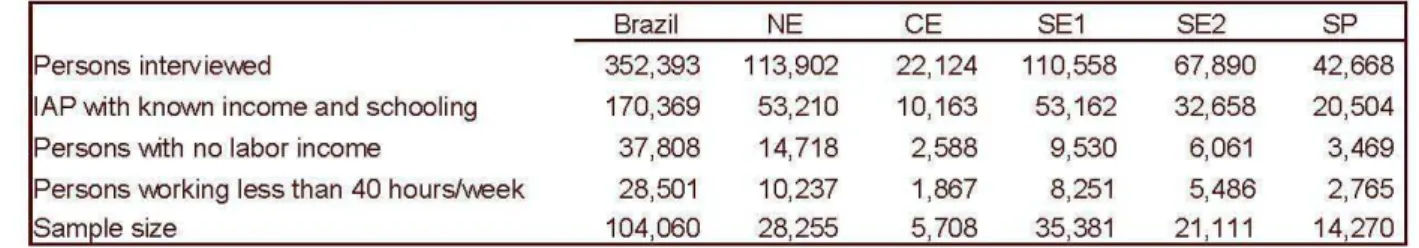
The following tables present the sample used by regions/state of interest and the main descriptive statistics, which were calculated considering the weighting of each individual.
Table 3 - Number of Interview Subjects per Region/State
Brazil NE CE SE1
Persons intervievved 352,393 113,902 22,124 110,558
IAP vvith known income and schooling 170,369 53,210 10,163 53,162
Persons vvith no labor income 37,808 14,718 2,588 9,530
Persons VvOrking less than 40 hourslvveek 28,501 10,237 1,867 8,251
Sample size 104,060 28,255 5,708 35,381
Table 4 - Descriptive Statistics of the Selected Sample
(in R$) Brazil NE CE SE1 SE2 SP
I ncome frem labor
mean 572 358 338 676 554 775
standard deviation 905 704 697 977 866 1.055
Gini Coeff. 0.55 0.57 0.58 0.52 0.53 0.50
Log labor income
mean 5.81 5.3 5.21 6.04 5.83 6.22
standard deviation 0.96 0.95 0.98 0.9 0.9 0.85
Schooling (years) 6.4 4.6 4.5 7.3 6.9 7.8
Gini Coeff. 0.32 0.42 0.42 0.29 0.30 0.27
Table 4 shows that the higher the average income, the less is the income and schooling inequality, measured here by the Pearson variation coefficient and the coefficient of Gini. This permits us to raise the hypothesis that the inequality of income and schooling are strongly correlated, and in turn smaller in the richest regions/states. The average schooling in the poorest regions is nearly 3 years less than in the richest ones. Indeed, we can see that income is directly proportional to schooling, which strengthens the hypothesis that the income differential can be explained by the difference in schooling leveIs.
SE2 SP
67,890 42,668 32,658 20,504
6,061 3,469
5,486 2,765
We computed for each region/state the median of the logarithm of income by leveI of schooling. The schooling x income curves, also known as Mincer curves, are
plolled in Graphs 3(a) and 3(b). One can see lhal lhe marginal relum of schooling
is rising for schooling leveIs above 10 years, unlike observed in developed countries with high leveIs of schooling among the general population.
Graph 3(a) - Schooling x Income
M セ MMM セ MM セMMM セ MMM セ MM セMMM セ MMM セ M⦅N⦅MMMMMMMMMMMMMMMMMMMMMMMMMMM
4 5
4 10 11 12 13 14 15
Years or Schooling
Graph 3(b) - Schooling x Income
80 セMMMMMMMMMMMMMMMMMMMMMMMMMMMMMMMMMMMMMMMMMMMMMMMMMMMMMMMMMMMMML@
7 5
êi 70
..
セ@ 65 o
o
.E 6 .0
l!
セ@1ij 5.5
li
::E 5.0
4 5
--- b J ---
... SP___ セ ce@ _______________________________________ _
- - - -
-4 6 7 8 9
Years or Schooling 10 11 12 13 14 15
Although we have data on a very large number of interview subjects, as can be seen in the last line in Table 3, the amount of information contained in these interviews is quite a bit lower than it appears. Income, besides being collected as a monthly integer value, was always reported in multiples of R$ 10 or the minimum
3.1
Methodology
We used a semiparametric model to construct the counterfactual density functions. These counterfactual densities were estimated from a sample generated by taking as a base the original sample and changing the attribute we wished to study, to see the impact of schooling on the distribution of income. The method comprises two steps: the first, parametric, which involves constructing the reweighting functions; and the second, non-parametric, which consists of estimating, based on kernel functions, the densily functions, as proposed by Rosenblall (1956) and Parzen (1962) .
Let
f
n be the density kernel estimator of densityf,
whose support is the variablew, based on a random sample of size n, {W11
w
2 ... , Wn }, with weighting 81, ... ,Bnlrespectively, and where Li Oi = 1. We then have:
(1)
where h is the window and K (-) is the kernel function. The most used kernels are the uniform, Gaussian and that of Espanechnikov, with the choice among them being an ad-hoc decision of the econometrician, who should keep in mind the nature of the variable whose density is being estimated. In this work, following the sug-geslions of DiNardo, Forlin and Lemieux (1996) and Bulcher and DiNardo (1998), we adopted the Gaussian kernel and worked with the logarithm of income to reduce the problem of asymmetry.
The choice of the window is an important point in estimating the kernel density, since there is a tradeoff between bias (difference between the estimated and real distribution) and variance: larger windows result in greater bias and less variance and vice-versa. There are various methods to select the window automatically, among them the cross validation and plug-in methods11. However, these methods are not adequate for data with the characteristics we are working with, since they are censured by intervals (grouped). The cross validation methods, for example, as pointed out by Silverman (1986), tend to generate inadequate results, h = O. Thus, we used visual selection, as detailed in Butcher and DiNardo (1998) : we began with a very narrow window (low smoothing), h = 0.05, and enlarged it until we obtained a smooth distribution, which turned out to occur at h = 0.12. We can justify this procedure of starting with a small window and increasing it by the belief that the human eye is better at smoothing than in the contrary sense (Butcher and DiNardo (1998)) . Underlying lhis melhod we are adopling lhe hypolhesis lhal lhe labor income distribution, and consequently the marginal productivity of labor, is smooth, which appears very reasonable given the large sample population. The choice of the lower bound of the windows that produce smooth distributions indicates that we prioritized bias over variance.
We estimated the counterfactual densities as proposed by DiNardo, Fortin and Limieux (1996), where reweighting functions are chosen for the sample. One can consider that each observation of the sample is a vector
(w,
z),
wherew
repre-sents wages (a continuous variable) and z the characteristics of each individual (we considered only education, measured in years of schooling) . Hence, we have joint density distributionsF(w,
z)
for income and education. The density of income for region 1, iRl(w),
can be written as the integral of the income density conditional on the leveI of schooling of the individuaIs,i
(w
/
z),
over the distribution of education,F
(z) :
fRl
(w)
1
dF(w, zlEw,z
セ@
RI)
zEO"
1
f(wlz, Ew
セ@
RI)dF(zIEz
セ@
RI)
zEO"
f(w; Ew
セ@RI, Ez
セ@RI)
(2)
where Oz is the domain of the set of attributes, Ez represents the region from where the education distribution is considered and Ew represents the region from where the income distribution is considered. To study counterfactuals, we are interested in modifying the structure of characteristics and 80 we define
f(
w; Ew = RI, Ez = RI)as the real income density of region 1 and j(w;Ew = Rl,Ez = R2) as the income density of region 1 if the education distribution were that of region 2 in the same period.
Under the hypothesis that the income structure of region 1,
f(wlz,
Ew = RI),does not depend on the distribution of education in region 2, we can write the hypothetical density
f(w;Ew
セ@RI,Ez
セ@R2)
as:f(w;Ew
RI,Ez
セ@
R2)
セ@
J
f(wlz,Ew
セ@
RI)dF(zIEz
セ@
R2)
J
f(wlz,Ew
セ@
RI)Wz(z)dF(zIEz
セ@
RI)
where W
z(z)
is a reweighting function defined by(3)
(4)
Equation (3) defines the income density in region 1 that would prevail if the educational conditions were similar to those of region 2, and as can be seen, is iden-tical to the definition in (2), except for the reweighting function
Wz(z).
In reality, the problem of estimating the desired counterfactual density function reduces to calculating the appropriate weightings. So, we can estimate counterfactual density functions using the method of weighted kernel density estimators where we use a new weighter that contains an estimate forWz(z).
Thus, we have,( 5)
where
L
Bi'ÍTz(Zi)
= 1 andSRl
is the set ofindices from the sample ofindividualsiESR l
of region 1. The differences observed between the real density of region 1 and the hypothetical density created represents the effect of a change in the education distribution.
One can see that by applying a rule ofBayes on (4), this quotient can be written as
() _pr--;(
e]Lコ]MMMセMMMM]rMMLMRQMKコI@Pr(
E z
セ@RI)
Wz z =
=-Pr(Ez
セ@RIlz) Pr(Ez
セ@R2)'
(6)
Since the leveI of education is a discreet variable that assumes a finite number of values, the estimation of
Wz(z)
by a probit model is equivalent to a simple counting.from reweighting by the schooling. Other methods of comparing estimated densities try to reduce their differences into a single number: the distance of Kullbach-Leibler, of Sibson, of Chernoff, difference between the standard deviations, differences be-tween percentiles, differences bebe-tween the percentile differentials (10-90, 10-50, 25-75, 5-95). [why does only lhis one nol add lo 10071 Ali lhese measures were used in this work. Besides this, we performed the Komogorov-Smirnov test of density inequalities.
4
Results
We applied the methodology described in the previous section and estimated the real distributions of the logarithm of income for the 5 sub-samples and for the full sample (Brazil), as presented in Section 3. Then, we estimated the counterfac-tual distributions for the Northeast and for Ceará, reweighting the samples by the schooling characlerislics of lhe Soulheasl Regions (SEI and SE2) and lhe slale of São Paulo. In this section we report and comment on the results for the state of Ceará, reweighted by the schooling of São Paulo, and for the Northeast Region, reweighled by lhe schooling of lhe Soulheasl Region (SEI and SE2). The resulls for the other cases are presented in the appendix.
Each of the graphs (4-6) below shows three densities: one counterfactual density, the real density from which this originated, and the real density of the region used in the reweighting12. The horizontal axis of the graphs is logarithmic.
Graph 4
Real densities for SEI and NE and counterfactual densities for NE with schooling of SEI
0 . 8 0 , - - - ,
0.70
MMMMMMMMMMMMセMMMMMMMMMMMMMMMM
セ@
- - -
-0.60
0.50
0.40
0.30
0.20
0.10
11 18 29 48 00 132 217 358 5éfj 973 1604 2644 4359 7187 11849 19536 work in come
Graph 5
Real densities for SE2 and NE and counterfactual densities for NE with schooling of SE2
0.80 ,---,
0.70
0.60
セ@
セMMMMMMMMMMMMMMMMMMMMMMMM
0.50
0.40
0.30
-0.20
0.10
-1 -1 18 29 4 8 80 132 217 358 590 973 16[14 2544 4359 7187 11 84 9 1953 6
work income
Graph 6
Real densities for SP and CE and counterfactual densities for CE with schooling of SP
0.80,---,
0.70 MMMMMMMMMMMMMMMMMセ@
êJ
@P]
- - -
MセMMMMMMMMMMMMMMMMMMMM
0.60
0.50
0.40 - - - - ICE/S p l
-0.30
0.20
0.10
11 18 28 4 8 80 132 217 358 590 973 16C14 2644 4359 71 87 11 84 9 19536
work income
We tested the equality between the original empirical distributions and their counterfactuals using the Kolmogorov-Smirnov test, in which the test statistic is the maximum oflhe difference belween lhe accumulaled densilies: max I F,
(w)
-
F2 (w )1.
We rejected the null hypothesis that the densities are equal at 1% significance in all cases, showing that the change in the schooling profile alters the income distribution. It is evident that the distributions1 3 are sensitive to the differences in schooling
and that the degree of sensitivity depends on the income percentile considered. The value of the minimum salary, R$ 136 at the time of the study, is the determining
13Read from the graphs:
factor in job income of workers in the Northeast, Ceará, and the Southeast (SE2) [SEI?], in view of the enormous concentration around this value in the distribution. The income distribution for the Southeast (SE2) is bimodal, with one of the modes corresponding to the minimum salary value and the other equal to the mode of lhe dislribulion for São Paulo, aboul R$ 300. The dislribulions for SP and SE1 are quite similar, which shows the significance of São Paulo on the aggregate of the Southeast Region. We can state, then, that in all states of the Northeast and Southeast, excepting São Paulo (SE2), the value ofthe minimum salary has a strong impact on the distribution of job income.
Comparing the tails of the counterfactual distributions with the original distri-butions, we see that they are quite dose, except for a rightward translation in the former ones. This is due to the direct proportionality between schooling and income together with the reweighting of the sample, whose effects on the income distrib-ution are similar to what would be obtained if we had added a schooling constant for each individual. One can observe that the central areas of the income distri-butions, which contain exactly the concentrations of most individuaIs and those whose income is near one minimum salary, change very little after reweighting. This behavior is explained by the fact that the wage structure is not altered in this process, overlapping [overpowering/overcoming?] the effect of the increase in schooling resulting from the same processo The mode, for example, remains equal to one minimum salary in all cases.
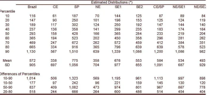
Table 5 presents some notable points (percentiles, means, standard deviations and percentile differences) of the estimated, real and counterfactual distributions. The support of [for?] the estimated distributions is the logarithm of income, which we limited for computational effects to the interval [1,10] with steps of 0.01. Based on these distributions, we constructed distributions, with the support being the leveI of income, simply taking the exponential of each point of the estimated distributions and renormalizing. We present in Tables a 1 and a 2 (in the appendix) the notable points of all the distributions constructed and the ratios of the percentiles of the estimated distributions.
Table 5 - Notable Points of the Estimated Income Distributions
Estimated Distributions (*)
Brazil CE SP NE SE1 SE2 CElSP
Percentile
10 116 61 187 70 144 125 87
20 147 90 250 101 196 153 125
30 189 117 302 124 250 192 147
40 237 136 358 141 299 235 183
50 293 158 428 166 365 284 233
60 365 194 523 202 450 358 296
70 469 247 672 262 572 459 412
80 665 334 916 365 796 639 639
90 1.130 567 1.510 639 1.339 1.086 1.200
Mean 572 338 775 358 676 553 584
SD 905 697 1.056 704 977 855 1.091
Differences of Percentiles
10-90 1.014 506 1.323 569 1.195 961 1.113
10-50 177 97 242 96 221 159 145
50-90 837 409 1.082 473 974 801 967
20-80 518 244 666 264 600 486 514
n
The values presenled were exlracled from lhe eslimaled (in log), laking lhe exponenlial of each poinl.The means and slandard devialions were calculaled direcllyfrom lhe reweighled sample wilh lhe income in leveI.
NE/SE1 NE/SE:
89 84
124 119
144 140
174 164
219 204
281 262
384 351
578 523
1.086 982
534 493
687 929
997 898
130 120
867 778
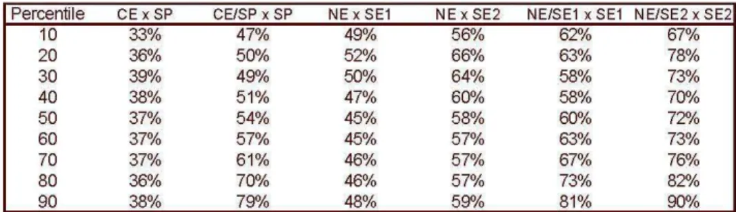
Table 6 - Income Ratio in the Percentiles
Percentile CE x SP CE/SP x SP NE x SE1 NE x SE2 NE/SE1 x SE1 NE/SE2 x SE2
10 33% 47% 49"10 56% 62% 67%
20 36% 50% 52% 66% 63% 78%
30 39"10 49"10 50% 64% 58% 73%
40 38% 51% 47% 60% 58% 70%
50 37% 54% 45% 58% 60% TZ'Io
60 37% 57% 45% 57% 63% 73%
70 37% 61% 46% 57% 67% 76%
80 36% 70% 46% 57% 73% 82%
90 38% 79"10 48% 59"10 81% 90%
Comparing the original distributions of Ceará and São Paulo, one can see that the income of the former is approximately 1/3 that of the latter in all the percentiles (Table 6) . On the other hand, in comparing the distribution of Ceará reweighted by the education of São Paulo with the original São Paulo distribution, we can see two effects: (i) there has been a gain in the income distribution of Ceará in all percentiles, and (ii) the gain increased as the income leveI (percentile) went up14. The growing marginal gain from schooling, illustrated in Graph 3, justifies the second effect, since individuaIs with more schooling, and consequently greater incomes, in receiving a " gain" in schooling by the reweighting effect, will have their incomes raised in a greater proportion than those with less schooling, whose income evolves little after an increase in schooling.
Comparing the Northeast Region with the Southeast, one can see that the first's income is between 45% and 50% of the second's for the SEI sample, and between 55% and 65% for the SE2 sample. After the reweighting, the same effects can be seen as when we compared the distribution Ceará with that of São Paulo. The effect of the reweighting is directly proportional to the difference between the original distributions, so it is greater in the case of CE x SP and less for NE x SE2, for all the percentiles. An interesting comparison is that the average income of the Northeast reweighled by lhe educalion of lhe Soulheasl (SE1) is 93% of lhe average Brazilian income . Here, like in the CE X SP comparison, the fact that schooling presents a rising marginal return justifies a greater income gain in the higher deciles.
The absolute gains are significant in all cases: in no decile is the income gain with reweighting less that 13% of the original income, and it reaches 70% in the ninth decile for the CE x SP comparison. The most relevant is that the income of Northeasterners is never less that about 60% of that of Southeasterners for the SEI sample and 67% for the SE2, and that in the upper deciles it comes quite near the income of Southeast residents if the two groups have the same leveI of education. The income in lhe ninlh decile of lhe NE reweighled by lhe schooling of lhe SE2 region reaches 90% of the SE2 income.
This facl is bel ler represenled in Graphs 7 to 9 (and A.4 lo A.6 of lhe appendix), where the counterfactual and the income distribution of the region/state that was used as a base for the reweighting approach each other at the higher income leveIs.
•
E
o
o
..
l!O
;:
Graph 7 - Evolution of Income by Percentile
for
CE, SP
andCE/SP
1,600 r - - - ,
1,400 - - -
-1,200 - - -
-1,000 - - -
-800
600
400
-200
セM
- -MセM
- --=-
---
=-
-=:-
- -
-=-
-:=-
- -
-=-
---
-= J
-10 20 30 4 0 50 60 70 80
Percentiles
Graph 8 - Evolution of Income by Percentile
for
NE, SE1
andNE/SE1
80
1,600 , -- - - ,
1,400
1,200
セ@ 1,000
O
o
.E 800
l!
セ@ 600 400
200
10 20 30 4 0 50 60 70 80
Percentiles
Graph 9 -Evolution of Income by Percentile
for
NE, SE2
andNE/SE2
90
1,200 r - - - ,
1,000
800
•
E
O
o
..
600l!
O
;:
4 00
200 MセMMMMセMMMMセMM セMMMセMMMセMMMMMMMMMMMMMMMM
10 20 30 4 0 50 60 7 0 80 80
Percentiles
"
___
="C"'E-'
-><-SP -A-CE/SP
-a-NE
_____ SE1
In Graphs 10 to 12 below, we present the difference between the two real dis-tributions and the difference between the counterfactual distribution and the real one whence it came15. These graphs allow us to visualize how much the income distributions approach each other after the reweighting by schooling.
Graph 10 - Difference of lhe Dislribulions (SE1 x NE)
0 . 4 0 , - - - ,
0.30
0.20
0.10
-0.10
-0.20
-0 .30
-0 .40
-0.50
MMMMMMMMMMMMMMMMiセセeイMMMMMMMMMMMMMMMMMMMMMMMMMMMMᆳ
セ@
MPNVPBMMMMMMMMMMMMMMMMMMMMMMMMMMMMMMMMMMMMMMMMMMMMMMMMMMMMMMMセ@
work income
Graph 11 - Difference of lhe Dislribulions (SE2 x NE)
0 . 4 0 , - - - ,
0.30
0.20
0.10
ッッッKM
セMM
MMMMMM
11 18セセセ
MMMMMMMMセ
セ セMMエ⦅MM
セ Z]]]
973 161J4セセセセ
26 (( 0 59MM
__
7187セ MMセ
118 ( 9 195Lェ@
-0.10
-0 .20
-0.30
-0 .40
-0.50
MP NVPBM MMMMMMMMMMMMMMMMMMMMMMMMMMMMMMMMMMMMMMMMMMMMMMMMMMMMMMMMMMMMセ@
wori< income
Graph 12 - Difference of lhe Dislribulions (SP x CE)
0 40 , - - - ,
0.3 0
________________
セ セ セセl@__
M⦅M⦅セ L ⦅セ@_____________________ _
0 .200 .10
-ッッッ エ MMセセ
セ セセセ\[Z[セセMMセMM
11 80 132セ セ[⦅⦅[[|セセ
973セセセ
16[14 26 HセセセZ⦅
4359 7187セ Z⦅セ@
Q QX セ Y@ 195-0.10
-0 .20
-0.30
-0 4 0
-0. 50
MoN V PセMMMMMMMMMMMMMMMMMMMMMMMMMMMMMMMMMMMMMMMMMMMMMMMMMMMMMMMMMMMMセ@
w ork incom e
We can see that the differences are negative at the lower income leveIs and posi-tive for the higher ones, which denotes that the preponderant effect is the difference of the average between the distributions rather than the difference of the dispersion. If this latter effect had prevailed, we would have seen positive differences in the tails and negative ones in the center of the support of the distributions.
We computed the distance between the distributions, before and after the reweight-ing, by the parametric measure known as the Kullbach-Leibler distance
(J) 16.
The results are shown in Table 7 below. Basically what this measurement does is rep-resent the a rea between two dist ribut ions where each a rea element (corresponding to eachw)
is weighted by the difference in density between the distributions. The effect of the w eighting is to introduce a non- linear relationship between the distance between the distributions, for each w, and its contribution to J. We find that more than 55% of the distances between Ceará and São Paulo and between the North-easl and SoulhNorth-easl regions (SE1 and SE2) are explained by schooling - 55.3% of lhe dislance belween São Paulo and Ceará and 55.0% (57.3%) of lhe dislance belween lhe Norlhe asl and region SE1 (SE2). This shows lhal more lhan half lhe income difference between the poorest region/state and the richest is due to the schooling differences of the population. We also computed the distance between the distrib-utions by the met r ics of Chernoff17 and Sibson18, suggested in Krzanow ski (2003),and obtained similar results, which are shown in Table 9.
16 The K ullbach-Leibler distance , J , is a measure of the divergence between two distributions . 17 The Cherno:lf distance between the distributions fI and f2 is defined as - log ..
Table 7 - Kullback-Leibler Dislances
Distance between the distributions
CE NE CE/SP CE/SE1 CE/SE2 NElSP NElSE1 NE/SE2
SP 1.5901 1.3826 0.7110 0.6700
SE1 0.9608 0.8031 0.3969 0.3611
SE2 0.5396 0.4127 0.2145 0.1761
% of the distance between the distributions explained by education
SP- CE 55.3% SP- NE 51.5%
SE1 - CE 58.7% SE1 - NE 55.0%
SE2 - CE 60.3% SE2 - NE 57.3%
We calculated the entropy coefficients of Theil and the concentration coefficients of Gini for the estimated distributions. These coefficients are measures of dispersion and are widely used as measures of inequality when applied to income distributions. The resulls are presenled in Table 8 below (and in Table
AA
in lhe appendix). In sum, we observed an increase in income inequality when we reweighted the sample. This is due to the fact that the rise in income is not uniform along the entire distribution, there being greater gains for the higher income leveIs.Table 8 - Gini and Theil Coefficients
Gini Theil
Coefficient Coefficient
Brazil 0.551 0.607
CE 0.582 0.768
NE 0.574 0.731
セ@ SE1 0.523 0.539
c
SE2 0.534 0.573
o
.",
0.505 0.498
v SP
'"
CElSP 0.622 0.797NE/SE1 0.608 0.766
NE/SE2 0.604 0.768
Remark: SE1 = MG + RJ + SP SE2=MG+RJ
fact that our exercise did not account for the change in the wage structure from the change in schooling, i.e., in general equilibrium this phenomenon would be observed partly or lolally.
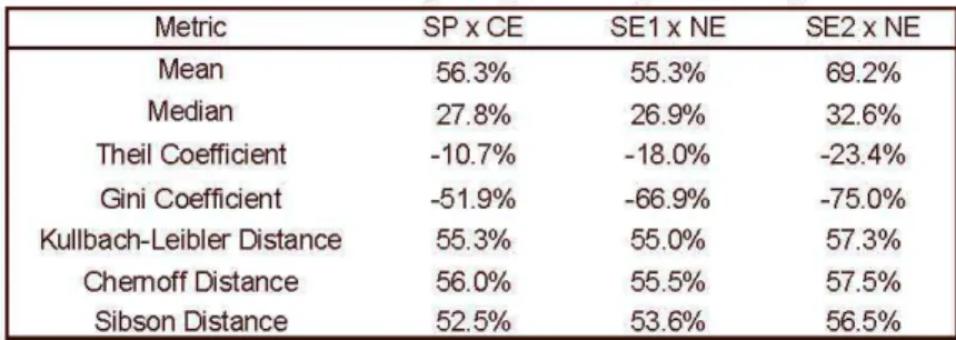
Table 9 - Percenlage Explained by Schooling
Metrie SP x CE SEI x NE SE2 x NE
Mean 56.3% 55.3% 69.2%
Median 27.8% 26.9"10 32.6%
Theil Coefficient -10.7% -18.0% -23.4%
Gini Coefficient -51.9% -66.9"10 -75.0%
Kullbaeh-Leibler Cistanee 55.3% 55.0% 57.3%
Chemoff Distance 56.0% 55.5% 57.5%
Sibson Distance 52.5% 53.6% 56.5%
We investigated the robustness of the results to the choice of window size by re-eslimaling ali lhe dislribulions wilh h セ@ 0.09 (-25% of lhe original h) and h セ@ 0.15 (+25%), and comparing the results against those obtained with the original value of h. We found that the changes in the results did not compromise them, even without observing a direct relation between the size variation of the window and the variation of the indicators presented in Tables 5 through 9.
It should be pointed out that the portion of the income difference explained by schooling is perhaps greater than shown in this work, since the cost of living is different in the regions. Services and nontradable goods are cheaper in the poorer regions, reflecting exactly the difference in wage leveIs, since these items tend to be more labor-intensive. The effect of correction by purchasing power in each region would be less in the lower income leveIs (consuming fewer services) and greater for individuaIs with higher incomes (consuming more services), accentuating the effect shown in Graphs 7 to 9.
5
Conclusion
In this work we sought to identify how much the income differential between the Northeast and Southeast regions and between the states of Ceará and São Paulo is explained by the differences in schooling leveIs of their populations. We used a semiparametric model to constrict counterfactual density functions, reweighting the individuaIs of the base region/state by the education distribution of the region of comparison. We estimated the distributions of real and counterfactual income of the state of Ceará and the Northeast Regions reweighted by the schooling leveIs of the Southeast Region and the state of São Paulo.
There are various factors that may be determining the income difference not ex-plained by the schooling differential, among them the life expectancy of the people, ethnic factors, the age structure of the population, quality of infrastructure, pres-ence/ absence of development stimuli and historical factors. A natural extension of this work would be, applying the method of counterfactuals, to decompose the income differential into some of these factors besides schooling, seeking to explain a greater portion of the income differentiaI. The relative importance of the above factors against the cost of eliminating them could well be of great value in orient-ing public policies to combat " regional inequality" . Other interestorient-ing extensions would be: (i) reweighting the income distribution of the Northeast Region by the schooling of Brazil without the North Region19; and (ii) reweighting the income
distribution of all regions by the schooling profile of Brazil as a whole, permitting determination of the size of regional inequalities controlling for schooling.
References
[1] Barros, Ricardo Paes de (1993). "Regional Disparities in Education Within Brazil: the Role of Quality of Education", Texto para Discussão nO 311, IPEA.
[2] Barros, Ricardo Paes de & Mendonça, Rosane (1995). "Os Determinantes da Desigualdade no Brasil", Texto para Discussão nO 377, IPEA.
[3] Barros, Ricardo Paes de, Camargo, José Márcio & Mendonça, Rosane (1997). "A Estrutura do Desemprego no Brasil", Texto para Discussão nO 478, IPEA.
[4] Blinder, Alan S. (1973). "Wage Discrimination: Reduced Form and Structural Estimates", Journal of Human Resources, 8, 436-455.
[5] Bourguignon, François, Ferreira, Francisco & Leite, Phillippe (2002). "Beyond Oaxaca-Blinder: Accounting for Differences in Household Income Distributions Across Countries", mimeo.
[6] DiNardo, John, Fortin, Nicole M. & Lemieux, Thomas (1996). "Labor Mar-ket Institutions and the Distribution of Wages, 1973-1992: A Semiparametric Approach", Econometrica, VoI. 64, No. 5, 1001-1044.
[7] Butcher, Kristin F. & DiNardo, John (1998). "The Immigrant and Native-Bom Wage Distributions: Evidence from United States Censuses", NBER Working
Paper Series 6630.
[8] Krzanowski, W. J. (2003). "Non-parametric estimation of distance between groups", Journal of Applied Statistics, Vol. 30, No. 7, 743-750.
[9] Oaxaca, R. (1973). "Male-Female Wage Differentials in Urban Labor Markets",
International Economic Review, 14, 693-709.
[lO] Park, B. U. & Marron, J. S. (1990). "Comparision of Data-driven Bandwidth Selectors", Journal of American Statistical Association, 85,66-72.
[11] Parzen, E. (1962). "On Estimation of a Probability Density Function and Mode", The Annals of Mathematical Statistics, 33, 1065-1076.
[12] Pessoa, Samuel (2000). "Existe um Problema de Desigualdade Regional no Brasil?" 1 mimeo.
[13] Rosenblatt, M. (1956). "Remarks on Some Non-parametric Estimates of a
Den-sity Function", The Annals of Mathematical Statistics, 27, 832-837.
[14] Sheater, S. J . & Jones, M. C. (1991). "A Reliable Data-based Bandwidth
Se-lection Method for Kernel Density Estimation", Journal of Royal Statistical
Society, 53, 683-690.
[15] Silverman, B. (1986). Density Estimation for Statistics and Data Analysis,
London: Chapman & Hall, 1986.
A
Tables and Figures
Graph A.1
Real densities for SP and NE and counterfactual for NE with schooling of SP
0 . 8 0 , - - - ,
0.70 - - -
Mセ@
セ@
0.60-El
- - - セMMMMMMMMMMMMMMMMMM
0.50
-0.4 0
-0.30
0.20
0.10
11 18 29 4 8 00 132 217 358 500 973 1W4 26 44 4359 7187 11 &1 9 19536
work inccme
Differences between the distributions of SP and NE (real and counterfactual)
0 . 4 0 , - - - ,
0. 3] _ _ _ _ _ _ _ _ _ _ _ _ _ _ MGセセ」⦅]]l@ ---=-=-==-=- ___________________ _
-0. 3J
-0.40
-o.w
MッN キ セMMMMMMMMMMMMMMMMMMMMMMMMMMMMMMMMMMMMMMMMMMMMMMMMMMセ@
Graph A.2
Real densities for SEI and CE and counterfactual for CE with schooling of SEI
0 . 8 0 , - - - ,
0.70
L
セ@
_______________ _
0.60
0.50
0 ( 0
-0.30
0.20
0.10
11 18 セ@ セ@ 80 132 セQ@
=
500=
L ⦅ セ ᆱ@ _ 9 n& 11 _ '_work in come
Differences between the distributions of SEI and CE (real and counterfactual)
0.40,---o====c---,
ISE1 - CE I
MMMMMMMMMMMMMMMMMMMMセMMMMMMMMMMMMMMMMMMMMM
-0 .10
」ャウセ・エGェ」セXcセBセQ@
c _______ _
-0. 20
-0 3J
-0.40
-0.50
セュセMMMMMMMMMMMMMMMMMMMMMMMMMMMMMMMMMMMMMMMMMMMMMMMMMMMMMMセ@
Graph A.3
Real densities for SE2 and CE and counterfactual for CE with schooling of SE2
0.80,-- - - ,
0.70
0.60
0.50 セMMMMMMMMMMMMMMMMMMM セ@
0 ( 0
-0.30
-0. 20
0.10
11 18 セ@ セ@ 80 132 セQ@
=
500=
L⦅セ ᆱ@ _9 n& 11_'_wcrk in come
Differences between the distributions of SE2 and CE (real and counterfactual)
0 . 4 0 , - - - ,
ISE2-CEI
MMMMMMMMMMMMMMMMMMMセMMMMMMMMMMMMMMMMMMMMMM
0 .10
-0 .10
-ISE2 - CE/SE21
-0. 20
-0 3J
-0.40
-0.50
セュセMMMMMMMMMMMMMMMMMMMMMMMMMMMMMMMMMMMMMMMMMMMMMMMMMMMMMMセ@
wcrk in come
Graph A.4 - Evolution of Income by Percentile
for
CE, SEI
andCE/SEl
1,600 , - - - ,
1,400
1,200
E
1,000 8E 800
セ@
,cc
セMMセMMMMMセMM
]]ZZZセ@
Percentiles
セ」・@
E
8
Graph A.S - Evolution of Income by Percentile
for
CE , SE2
andCE/SE2
1,20 0 , - - - ,
1.000
..!: 600
セ@
o
セ@
Percentiles
Graph A.6 - Evolution of Income by Percentile
for
NE, SP
andNE/SP
1,600 セ MMMMMMMMMMMMMMMMMMMMMMML@
1,400
1,200
1,000
, cc
セMMセMMMMMセZZMMMMMセMMMMM
]j MMMMM
Percentiles
セ」・@
_____ SE 2
---&-CE/S E2
Table A.I - Notable Points of the Estimated Income Distributions
Estimated Distributions(*)
Brazil CE SP NE SE1 SE2 CE/SP CE/SE1 CE/SE2 NE/SP
Percentile
10 116 61 187 70 144 125 87 82 77 94
20 147 90 250 101 196 153 125 122 116 128
30 189 117 302 124 250 192 147 143 137 148
40 237 136 358 141 299 235 183 172 162 183
50 293 158 428 166 365 294 233 219 204 233
60 365 194 523 202 450 358 296 279 260 302
70 469 247 672 262 572 459 412 380 344 412
80 665 334 916 365 796 639 639 578 513 633
90 1,130 567 1,510 639 1,339 1,086 1,200 1,108 1,002 1,176
Mean 572 338 775 358 676 553 584 547 503 569
SD 905 697 1,056 704 977 855 1,091 1,041 978 1,033
Differences of Percentiles
10-90 1,014 506 1,323 569 1,195 961 1,113 1,025 926 1,082
10-50 177 97 242 96 221 159 145 137 128 139
50-90 837 409 1,082 473 974 801 967 888 798 943
20-80 518 244 666 264 600 486 514 457 397 505
(' ) Th e valu es lXesenled were exlrocled I rom lhe eslim óted (in log), lél<ing lhe expooenl ial 01 each pu nI
The meoo s and slandard deviótions were calculaled 、ゥ イ・」ャセ@ I rom lhe イ ・キセ エャ ャ・、@ sampl e l'iilh lhe in com e in levei
NE/SE1 NE
89 124 144 174 219 281 384 578 1,086
534 687
Percentile 10 20 30 40 50 60 70 80 90 Percentile 10 20 30 40 50 60 70 80 90
Table A.2 - Income Ratio in the Percentiles
CExSP CE/SP x SP CE x SE1 CE x SE2 CE/SE1 x SE1
33% 47% 42% 49% 57%
36% 50% 46% 59% 62%
39% 49% 47% 61% 57%
38% 51% 45% 58% 58%
37% 54% 43% 55% 60%
37% 57% 43% 54% 62%
37% 61% 43% 54% 66%
36% 70% 42% 52% 73%
38% 79% 42% 52% 83%
NExSP NE/SP x SP NE x SE1 NE x SE2 NE/SE1 x SE1
38% 50% 49% 56% 62%
41% 51% 52% 66% 63%
41% 49% 50% 64% 58%
39% 51% 47% 60% 58%
39% 54% 45% 58% 60%
39% 58% 45% 57% 63%
39% 61% 46% 57% 67%
40% 69% 46% 57% 73%
42% 78% 48% 59% 81%
Table A 3 - Coefficients of Gini and Theil
Brazil
CE - O>
NE
(Il .!:
c
-.- セ@
SE1
Nセ@ O)
ッセ@
SE2セ@ SP
c o .",
"
CE/SPv
'"
.oCE/SE1
o>C
c o
Zeセ@ CE/SE2
o>U
.-v", セ@ NElSP
セキ@
v NE/SE1
'"
NE/SE2Remark: SE1
=
MG + RJ + SP SE2=
MG +RJGini Theil
Coefficient Coefficient
0.551 0.607
0.582 0.768
0.574 0.731
0.523 0.539
0.534 0.573
0.505 0.498
0.622 0.797
0.621 0.805
0.618 0.810
0.609 0.760
0.608 0.766
0.604 0.768
CE/SE2 x SE2
61% 76% 71% 69% 72% 73% 75% 80% 92%
NE/SE2 x SE2
67% 78% 73% 70% 72% 73% 76% 82% 90%
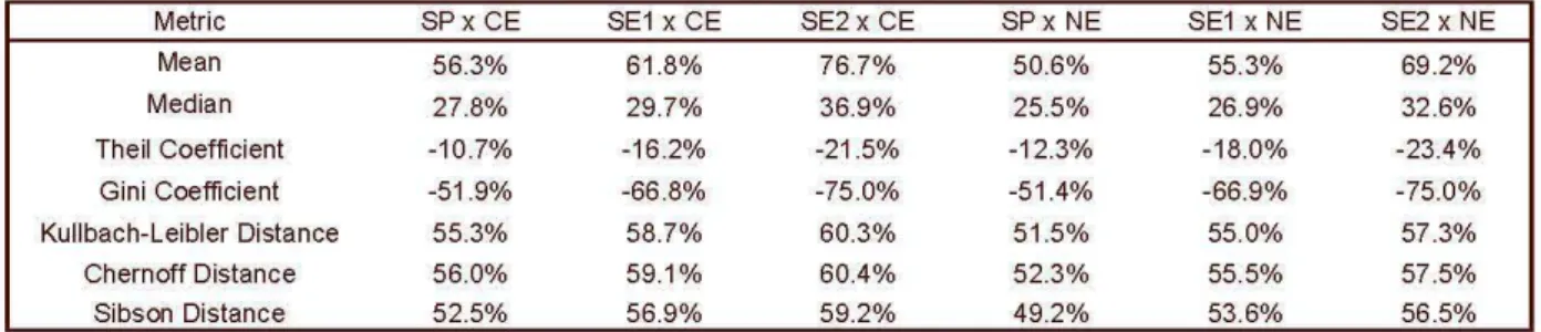
Table
AA
-
Percentage Explained by SchoolingMetric SPx CE SE1 x CE SE2 x CE SPx NE
Mean 56.3% 61.8% 76.7% 50.6%
Median 27.8% 29.7% 36.9% 25.5%
Theil Coefficient -10.7% -16 .2% -21.5% -12.3%
Gini Coefficient -51.9% -66.8% -75.0% -51.4%
Kullbach-Leibler Distance 55.3% 58.7% 60.3% 51.5%
Chernoff Distance 56.0% 59.1% 60.4% 52.3%
Sibson Distance 52.5% 56.9% 59.2% 49.2%
SE1 x NE SE2 x NE
55.3% 69.2%
26.9% 32.6%
-18.0% -23.4%
-66.9% -75.0%
55.0% 57.3%
55.5% 57 .5%