The effects of openness on industrial employment in Brazil

(1)

r - - - ＭＭＭＭＭＭＭＭｾＭＭＭＭＭＭＭＭ

-, . . #-,"FUNDAÇÃO

, . .

GETULIO VARGAS

EPGE

Escola de Pós-Graduacão em

_-'

Economia

· "THE EFFECTS OF OPENNESS

ON INDUSTRIAl.

ElVIPLOYMENT IN BRAZIL"

GUSTAVO GONZAGA

(Pue/RJ)

LOCAL

Fundação Getulio Vargas

Praia de Botafogo, 190 - 10° andar - Auditório

DATA

07/11/96

(SU

feira)

HORÁRIO

16:00h

(2)

i

..

The Effects of Openness on

Industrial Employment in Brazil \

Gustavo M Gonzaga

Departamento de Economia

PUC-Rio, Brazil

Preliminary Version

October 1996

*

(3)

• ..

Resumo

Este artigo tem dois objetivos pnnClpms. Primeiramente, apresentamos as pnnClpms

evidências de que a baixa qualidade do emprego é o maior problema do mercado de trabalho

brasileiro. Mostra-se que o país tem absorvido um crescimento da oferta de trabalho significativo

ao longo dos últimos anos sem registrar um aumento da taxa de desemprego. No entanto, os postos

de trabalho no Brasil são, em média, extremamente precários. Em grande medida, a precariedade do

emprego no Brasil está relacionada à alta rotatividade da mão-de-obra, que desincentiva o

investimento em treinamento, impedindo o crescimento da produtivid::;de do trabalho. De acordo

com os indicadores passíveis de comparação internacional, o Brasil apresenta uma das maiores

taxas de rotatividade do mundo.

Em segundo lugar, estuda-se a evolução recente do emprego industrial, uma vez que o setor

industrial está tradicionalmente associado à geração de bons empregos no Brasil. Mostra-se que o

nível de emprego industrial tem se reduzido de forma praticamente contínua desde o início desta

década. A estimação de um modelo de ajustamento parcial do emprego nos permite explicar este

fenômeno. Mudanças estruturais significativas na elasticidade custo salarial do emprego e no

coeficiente de tendência são detectadas a partir do início da década de 90. Um simples modelo

teórico é usado de forma a interpretar estas mudanças estruturais como a resposta ótima das

empresas industriais ao ambiente de maior competição externa, devido à abertura comercial. Isto,

junto com o uso crescente de tecnologias poupadoras de mão-de-obra, são suficientes para explicar

a brutal queda do emprego industrial no Brasil ao longo dos últimos seis anos .

(4)

I. Introduction

This article has two main objectives. The first one is to ｣ｨ｡ｲ｡ｾｴ･ｲｩｺ･＠ the behavior of the

Brazilian labor market over the more recent years. The idea is to identify current trends in some key

labor market indicators, and reversals that could be attributed to structural reforms.\ The findings

.. of some recent articles that the main Brazilian labor market problem seems to be the bad quality of

jobs, and not lack of job creation, are confirmed here. It is shown that the occupied population has

i

been growing faster than total population without exerting significant pressure on the

unemployment rate. Since the Brazilian economy has grown less than the nurnber of job positions

over the last fifteen years, labor productivity has decreased. The productivity reduction has been

reflected in a decline of the quality of Brazilian jobs, on average. In fact, the quality of Brazilian

jobs is very low. This is illustrated in several dimensions: low pay, low productivity growth, high

tumover, high number of informal jobs, and a significant reduction in the proportion of industrial

jobs.

Given the importance ofthe industrial sector in providing good jobs, the second objective of

this paper is to study the evolution of industrial employment over the laSt eleven years. It is shown

that the leveI of industrial employment has significantly declined in an almost continuous fashion

since the beginning of this decade. The estimation of a partial adjustment labor demand equation

for the industrial sector allows us to provide an explanation for this decline. A significant structural

change in the main parameters of this equation is detected in the beginning of this decade. A simple

theoretical model is used to interpret the structural change as an optimal response of

profit-maximizing industrial firms - mostly, producing traded goods - to a more open environment to

foreign competition. This, coupled with the effects of an increase in the use of job-saving

technologies, such as outsourcing and downsizing, is able to explain the recent evolution of

industrial,employment in Brazil.

(5)

•

The paper is organized as follows. The next section characterizes the functioning of the

Brazilian labor market over the last fifteen years. It presents and discusses data on job creation, job

quality and income inequality. The third section presents a dynamic labor demand model in which

the revenue function of profit-maximizing finns depends on the degree of market power. The

assumption that the degree of market power is affected by the degree of openness is the main source

of structural change in the labor demand equation. Section 4 estimates a partial adjustment labor

demand equation for the Brazilian ｩｮｾｵｳｴｲｩ｡ｬ＠ sector. It is shown that 'the key parameters of the

equation changed significantly over the more recent years. This is interpreted as a natural response

of industrial finns to a more competitive environrnent, coupled with the effects of an increasing use

of job-saving organization technologies.

11. Characterization ofthe Brazilian Labor Market Problem

In Amadeo et ai. (1994), Amadeo and Gonzaga (1995) and Gonzaga (1996b), the Brazilian

labor market was characterized as one with a high capacity of job creation, but with a poor quality

of the jobs created, on average. The problem of the Brazilian market, thus, seems to be a problem of

job quality, rather than one of quantity. In this section, I review and update the main Brazilian labor

market indicators that confinn this diagnostico

Table 1 below presents some selected data, taken from the two main FIBGE household

surveys: the Pesquisa Mensal de Emprego (PME) and the Pesquisa Nacional por Amostras de

Domicílio (PNAD), and from the National Accounts. The evidence point to a labor market which is

capable of absorbing a growing number of people without generating an increase in the open

unemployment rate.

Table 1: Brazil - High Capacity of Job Generation Main Indicators of Job Creation

A verage Annual GNP Growth (National Accounts, 1980-95)

A verage Annual Total Population Growth (National Accounts, 1980-95)

A verage Annual Occupied Population Growth (PNAD,1981-95)

4

2,0%

1,6%

(6)

i

Average Unemployment Rate - Six Main Metropolitan Regions (PME, 1982-95)

A verage Participation Rate (PNAD,1981-95)

5,3%

53,4% (81) - 61,3%(95)

On average, Brazil increased by 3.1 % a year its occupied population in a 14-year period, which rose from 45.5 millions in 1981 to .69.6 millions in 1995, and accumulated a 53% increase

over the whole period. The labor force has also increased significantly in that period, from 47.5

million workers in 1981 to 74.1 millions in 1993. The participation rate increased from 53.4% to 61.3% between 1981 and 1995, reflecting mostly a growing trend of female participation in the

labor market, from 32.9% to 48.1 %.

This increase, however, could be accommodated without a rise in the unemployment rate,

which confinns that the Brazilian labor market is able to create a large number of new job

opportunities. In fact, the average unemployment rate in the six main metropolitan regions in Brazil between 1982 and 1995 is 5.3%. It rarely exceeded 6 percent over that period. This is relatively

low, by intemational standards. Data from CEP AL (1995), for example, show that Brazil had the second lowest urban unemployment rate in South America in 1994. The average European

countries' unemployment rate in 1995 was above 10%.

The surprising aspect of these numbers is that the Brazilian economy did not grow much

over that period. Table 1 shows that the average mmual growth of Brazilian GNP was around 2% between 1980 and 1995, only slightly more than annual population growth, which was 1.6%, on

average.

What could explain the fact that an ailing economy, such as Brazil's over the last fifteen

years, was able to create so many new job opportunities? The answer lies in the poor quality of the jobs created. In general, a bad job is characterized by low pay, usually a result of low productivity.

Therefore, low pay should be viewed as the most important symptom of a bad job. However, this

infonnation can be ｣ｯｾｰｬ･ｭ･ｮｴ･､＠ by some other indicators, since bad jobs are also characterized by bad working conditions. Table 2 below presents some indicators that are usually associated with

(7)

•

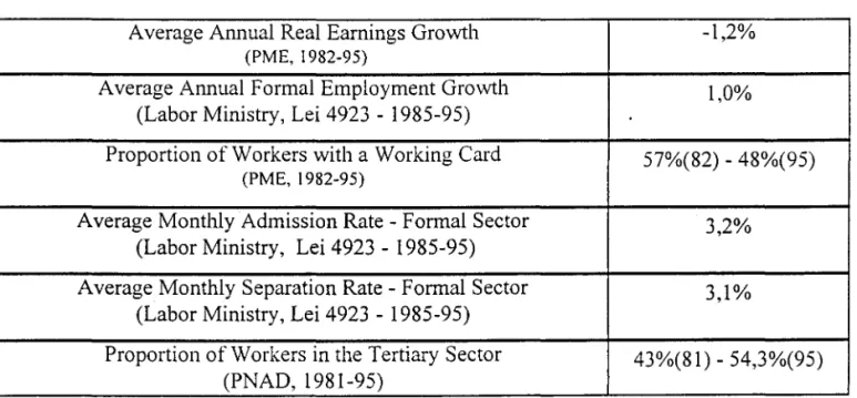
On average, a job in the six main metropolitan regions in Brazil paid 10% less at the end of

1995 than in the beginning of 1982, in real terms. If we compare annual averages, the decrease was

even more pronounced: 14% between 1982 and 1995, an average annual falI of 1.2%.

This happened mainly as a result of the significant reduction in the proportion of formal

jobs and industrial jobs. The prop011ion of workers with a formal contract (com carteira assinada,

with a working card), and therefore covered by the Brazilian Labor Code (Consolidação das Leis

do Trabalho, CLT), in non-agriculture activities decreased from 57% in 1982 to 48% in 1995, and

to 46.3% by mid-1996?

Table 2: Brazil - Bad Jobs Job Quality Indicators

A verage Annual Real Earnings Growth

(PME, 1982-95)

A verage Annual Formal Employment Growth (Labor Ministry, Lei 4923 - 1985-95)

Proportion of Workers with a Working Card

(PME, 1982-95)

Average Monthly Admission Rate - Formal Sector (Labor Ministry, Lei 4923 - 1985-95)

Average Monthly Separation Rate - Formal Sector (Labor Ministry, Lei 4923 - 1985-95)

Proportion of Workers in the Tertiary Sector (PNAD,1981-95)

-1,2%

1,0%

57%(82) - 48%(95)

3,2%

3,1%

43%(81) - 54,3%(95)

Data from the Labor Ministry confirm that working card employment increased very little

over the last eleven years. While occupied population increased from 55,4 millions in 1986 to 69,6

millions in 1995 (an average annual growth of2,6%), formaljobs increased only by 1% a year, on

average, between 1985 and 1995. The absolute number of formal jobs by mid-1996 was about the

same size as in 1990. This means that most of the reduction in the proportion of formal jobs in the

occupied population happened after 1990. This suggests that Brazilian firms responded to the

2 Workers hired under a formal contract, have a working card signed, which entitles them to receive social security

(8)

•

increase in externaI price competition, a result of the removal of many import non-tariff barriers, by

informalizing their labor force.

Labor turnover in the formal sector, on the other hand, is high when compared to other

countries, suggesting little worker-firm attachment (and, therefore, little on-the-job training) even in

the formal sector of the economy. Approximately 730 thousand workers (3.2% of the formally

employed), on average, got a new formal job each month between 1985 and 1995, while about 720

thousand (3.1 % of the formally employed), on average, lefi their formal jobs each month during the

same período Only a few countries collect data on gross labor turno ver, which makes it hard to put

these numbers in perspective.

However, there is another labor turnover measure, available for the Brazilian formal labor

market, which allows us to make international comparisons. This is the proportion of workers with

less than two years of tenure at the same job. The higher this measure, the higher is labor turnover.

Data from the Labor Ministry (RAIS, Relatório Anual de Informações Sociais) show that,

on average, in the period 1988-1992,49% ofBrazilian formal workers remained less than two years

in the same job. How does this number compare to those available for other countríes? The answer

is in Table 3 below, which shows the same measure for several other countries, for the industrial

sector only. The years vary across countries, and correspond to the most recent available figures.

The Table shows that Brazil presented the highest leveI of labor turnover.

Table 3: Labor Turnover in Several Countries

Proportion ofIndustrial Workers with less than Two Years ofTenure

Belgium 18%

Germany 21%

Denrnark 27%

France 22%

Ireland 22%

Italy 13%

(9)

•

Netherlands 28%

Canada 33%

United States 39%

Finland 28%

Brazil 47%

Note: Source of data for other countries - Nickell, 1995 .

Gonzaga (1996b) shows that this measure of labor turnover decreases significantly with

education (completed years of study) and with the size of establishments. It is also shown that

tumover does not reduce significantly if one considers only workers with more than 25 or 30 years

of age. The implications are that Brazilian firms do not keep a long-term relationship with their

workers, specially with low-educated workers.

Investment in training is a risky joint investment. since the appropriation of the investment

retums is uncertain. A higher labor tumover increases this risk, since it increases the odds that

workers trained would leave the firm and use the benefits of this training in other firms.3 This

implies very little on-the-job-training. The result is a low equilibrium for the society, characterized

by high tumover, low investment in training, low productivity growth, and poor quality of jobs.

Another piece of evidence regarding the poor quality ofthe new jobs created in Brazil in the

last fourteen years is given by a sectoral decomposition of employment. The proportion of workers

employed in the tertiary sector, for example, increased from 43% in 1981 to 54.3% in 1995. This is

a matter of concem, since the typical service sector job in Brazil is held by the relatively unskilled,

does not provide a formal contract, is not unionized, and has a short tenure. Amadeo et aI. (1993)

show that approximately 60% of workers employed in the services sector in the beginning of the

90s have 4 years or less of education. By contrast, the proportion of workers with 4 years or less of

study in the industrial sector is around 40%, while for the whole economy is near 50%. Moreover,

about 38% of employees in the services sector in the beginning of the 90s have a formal contract

(have their working cards signed). The corresponding figure in the industrial sector is around 85%.

3 Gonzaga (1996b) discusses how some Brazilian labor market institutions act as incentives for higher labor

(10)

Most of these service sector jobs display low tenure: 47% of employees have less than one year of

job experience at the firmo In the industrial sector, the proportion is 31 %.

Even among formal workers, tumover rates are much higher in the service sector. In the

commerce sector, for example, approximately 4.2% 01' formal1y employed workers, on average, got

a new job each month between 1989 and 1995. The corresponding figure in the industrial sector is

3.2%. The tertiary sector is also characterized by low unionization rates. Amadeo and Camargo

(1993) show that the proportion of workers that belonged to a union in 1986 was 29.1 % in the

manufacturing sector, compared to 5.6% in the service sector and 14.4% in commerce.

Table 4 shows some evidence that income inequality in Brazil, one of the worst in the

world, deteriorated in the last decade. Amadeo ef aI. (1994a) show that the income ratio of the

richest 10% against the poorest 40% in Brazil is around 6, while for other countries with population

over 5 million and good quality data this ratio is below 3.5. The rise in income inequality is

illustrated by the time series behavior of the national Gini coefficient in the 1980s, which increased

from 0.564 in 1981 to 0.602 in 1990, after reaching a peak of 0.630 in 1989 (data from PNAD,

FIBGE). Barros and Mendonça (1994) present additional evidence that Brazilian income

distribution worsened in the 1980s. They show that all tenths of the distribution lost income in the

1980s, but the poorest were the most affected. While average income declined by 1.5% a year, on

average, between 1980 and 1990, the mean income of the 10% poorest decreased by 5.1 % a year,

on average, in the same period. The 1 % richest, on the other hand, increased their income share

from 12.1% in 1981 to 13.9% in 1990.

Table 4: Brazil - Income Distribution - 1980s

Gini Coefficient 0.564 (1981) - 0.602 (1990)

A verage Mean Income Growth: -5.1 % a year

10% Poorest

A verage Mean Income Growth: -1.4% a year

(11)

The Gini coefficient for the years 1992, 1993 and 1995 ｷ･ｲｾ＠ 0.571, 0.601 and 0.565,

respectively. This shows an erratic behavior of income distribution in Brazil in the 90s. However,

the significant drop in inequality after the Real Plan indicates that the success in bringing down

inflation from an average of 45% a month to an average of 1.5% a month had a significant impact

on lifting living standards of the poorest in Brazil. This is a consequence of the fact that workers

eaming less than two minimum wages in Brazil have little protection against the inflationary tax,

since in general they have no access to indexed banking accounts.

111. Dynamic Labor Demand Models and Employment Adjustment Costs

In this section, I discuss the general framework of dynamic labor demand models and the

lssue of employment adjustment costs. I then propose one way by which openness affects

employment determination. This is done by considering a monopolistic competition setup, which

implies that revenues depend on price-setting dynamics. Openness is assumed to produce an

increase in the price elasticity of product demand, since more firms compete in the domestic market

in a more open environment . The assumption is that the transition from a closed economy to an

open economy does not imply a transition from an imperfectly competitive economy to a perfectly

competitive economy, which is usually assumed in open economy models. The direction here is the

same, that is, to increase the degree of price competitiveness. However, it is assumed that domestic

firms still carry a certain degree of monopoly power after the removal of import tariff (and

non-tariff) barriers.4 This allows us to evaluate the effect of changes in the degree of monopoly power

on labor demando

The increase in the price elasticity of product demand is shown to increase, in absolute

terms, the wage elasticity of labor demando This is easily shown in the static condition for profit

maximization without costs of employment adjustment, which states that marginal revenue equals

marginal cost. This condition, in the price-setting setup, implies that factor demand price elasticities

depend on the product-demand price elasticity. In the dynamic frame\vork, when one allows for

4 Cruz (1996) computes that the average nominal import tariff in the manufacturing industrial sector in Brazil has

(12)

employment adjustment costs, the Euler equation is highly non-linear, as shown in Burda (1991). In

the next section, a partial adjustment equation is used to test these implications ofthe mode1.5

The idea is to motivate the estimation of dynamic labor demand equations for the industrial

sector in Brazil. The arguments in this section will be used as the theoretical background to test

whether there were significant structural changes in any of the key parameters that could be

explained by the opening of the economy. In what follows in this section, I briefly discuss the

general reasoning for considering dynamic labor demand models, and how the introduction of

imperfect competition affects the Euler equation in these models.

The conventional view of how labor markets function in modem economies is one in

whichjobs usually last more than one day. In general, contracts between workers and firms are not

reviewed every day. In most cases, relationships actually last for a considerable length of time. A

major reason for this is the existence of non-trivial costs 01' hiring and firing workers. It has long

been recognized that the firm's profit maximization problem should then be solved in an

intertemporal framework that considers explicitly these labor tumover costs.6 The general

maximization problem in a dynamic labor demand model is set as:

00

Max

E'L

e

i(R(Z'+i,N'+i)- Wt+iN'+i - C"(N'+i - N t+i-I ))

i=O

where EtC.) denotes expectations formed at time t; O < 8 < 1 is a real discount factor assumed to be

constant for analytical simplicity; R(.) is a revenue function that depends on Nt, the employment

leveI, and on Zt , an index of product demand conditions; W_tis the real wage rate taken as given by

the firm; and C(.) is the tumover cost function, which depends on the size of employment

adjustment.

The standard assumption regarding the structure of adjustment costs, the C(.) function, is

that it is strictly convex (usually, quadratic) and symmetric. It showed up first as a matter of

5 It is important to mention that only partia I equilibrium effects are being considered here. without any effort to derive a

general equilibrium model.

(13)

•

analytical convenience and it is still present in most dynamic labor demand models. The intuition

behind the quadratic structure is that the introduction of new hires in a workplace could be more

disruptive the greater the size of the change. The costs of hiring new workers would thus increase

more than proportionally with respect to the number of workers hired. Conversely, laying off

several workers at once is also in general felt more intensively the larger the adjustment.

The quadratic structure implies that the Erm adjusts slowly its labor input towards the

desired employment leveI. It spreads the employment adjustment over time, approaching gradually

and asymptotically each new target leveI. This gives the basis for the traditional employment partial

adjustment equation, which one obtains from solving the maximization problem above, assuming

quadratic adjustment costs, and a linear-quadratic (on labor) revenue function:

Nt = a

+

À Nt-1

+

ｾ＠ (L) Ft

+

Et ;

where F is a vector of forcing variables (such as W, Z, and real revenues), À is a coefticient, and

ｾＨｌＩ＠ is a lag polynomial, with coefticients given by a linear combination of the parameters of the

model.7

Now, instead of assuming a linear-quadratic revenue function, consider an economy with a

representative Erm that uses labor as its only factor of production, according to a production

function given by Y_t= At

Nt

,

where At is a technology component, and O<a<l. The representative

firm has some monopoly power and faces a constant-elasticity product demand curve given by

y,

=

ｚｊｾＭｉＯＨｉＭｊＮｬＩ＠ , where Zt is an index of product demand, P_tis the firm's price, and 0<1-1<1 is the

inverse of the mark-up factor. Note that the perfect competition case is nested in this formulation,

being observed when 1-1 = 1, which implies an infinite product-demand price elasticity.

The parameter 1-1, therefore, is an index of price competitiveness. The doser it gets to 1, the

higher is the number of firms competing in the representative firm's product market. One can then

examine the effects of openness on employment determination through its effects on the parameter

7 The main alternative to the standard quadratic structure of C(.) is to assume that turnover costs are linearly related

to the size of adjustment. i.e., that turnover costs are fixed per worker hired or fired. The result is that the firm does

(14)

1-1. The idea is that the reduction in import tariffs (or the removal of non-tariff barriers) increases the

number of firms competing in the domestic market. This can be modeled as an increase in the price

elasticity of product demand, which would imply a decrease in the mark-up factor, i.e. an increase

in 1-1.

The revenue function implied by combining the production function and the product

demand function above is given by:

R = Z (1-J.l) A J.l N aJ.l

I I I I

The firms' profit-maximization problem is thus given by:

00

Max E,

L

8 i (ZII:t

_{ａｉｾｩｎ＠}

Il':i - WI+iN I+i - C(N I+i - N I+i-I))

i=O

The static labor demand condition is found by setting CC.) = O above, i.e. by deriving the

model without considering costs of employment adjustment. The solution (in logs) for each period t

is then given by:

In

N

_I = ---(in

-1

W_I- ｉｮＨ｡ｾｬＩ＠ - (1- ｾｬＩ＠ In Zt - ｾｬ＠ In AI)

1- ｡ｾ＠

Note that the wage elasticity of labor demand is -lI(l-al-1). Therefore, an increase in price

competitiveness, represented in this model as a rise in the parameter 1-1, increases the

employment-wage elasticity, in absolute terms. The reduction in rents, caused by the more open environrnent,

decreases the steepness of labor demand curves. In other words, wage increases cost more jobs in

the open economy.

Burda (1991) derives a non-linear dynamic labor demand equation in the monopolistic

competition setup. The fact that the wage elasticity of labor demand increases is still valid in the

case of non-zero adjustment costs. The process is shown to have richer dynamics than in the partial

adjustment case and to depend on how expectations about future wages and product demand

(15)

•

In the next section, I estimate a partial adjustment labor demand equation in order to test

whether the labor cost elasticity of labor demand increased afier the opening period in the Brazilian

industrial sector.

IV. Structural Breaks in Industrial Employment Determination in Brazil

As we have seen in the first part of this paper, the main problem of the Brazilian labor

market seems to be the low quality of jobs, not lack of job creation. Therefore, a legitimate concern

of the Brazilian society lies on the ability of the economy in generating good jobs. Since most of

the good jobs are in the industrial sector, I study this sector more c1osely. In particular, the objective

of this section is to estimate a partial adjustment labor demand equation for the Brazilian industrial

sector.

In" general, industrial jobs are, on average, better than others jobs in Brazil . They usually

offer higher pay, a higher percentage of workers is formally hired (the employers sign the working

card), and the leveI of turno ver is lower. However, the industrial sector in Brazil has reduced its

relative employment share over the last fifieen years. Data from PNAD (Pesquisa Nacional de

Amostras por Domicílio), FIBGE, reveal that the share of workers on the manufacturing industry

fell from 15% in 1981 to 12.3% in 1995, with most ofthe reduction happening afier 1990. The

result is a deterioration of the average quality of employment in Brazil.

Data from PIM (Pesquisa Industrial Mensal), a monthly industrial establishment survey

from FIBGE, show that between 1985 and 1995, industrial production increased by 1.3% a year, on

average, accumulating a total increase of 14% over the whole period (see Graph 1).8 However,

industrial employment fel! by 1.9% a year, accumulating a total reduction of 17.8% in the same

period. In fact, Graph 1 shows that there is an almost continuous trend of industrial employment

reduction since the beginning of this decade. This suggests that the relation between production

growth and employment growth worsened over the recent years.

8 The data source is PIM, from which it is possible to construct series of employment, production and average real

(16)

0,3

0,2

0,1 .

°

_.

-0,1 "',

-0,2

-0,3

li)

co

C _co

-, I , li) co C :l -, .'

.

'\ I \ 1 \ '

' . \ I

li)

ｾ＠ <O co C:

o

o-Z o<:(

I,

Graph 1: Industrial Employment and Production Seasonally Adjusted - 1985-96

.. I'·

• , " UI

I , I' •

" ,

I '

"

.

I

..

... '\. " ....

\ , '"

,

, , I ' I '\ • "

I , ,

r , I

I " " " I r I

' " I

"

\ .'\

I,

,i

.

• I

\ , ,

.

\ ,," \ '

I •

- I

..

r", \ I

,"

- -_ .. _-

-_._._----<O r--.

....

r--. co co O> O> o o o _Oi ｾ＠ N N N M M ｾ＠ｾ＠ｾ＠ｾ＠ _ｾ＠ co co co co O> O> O>

ｾ＠ O> _52? O> _52? O'l m

o- .o _:i >. :;:,

ｾ＠ o, c c ;; C: :a :i u >- :;:, C:

QJ QJ QJ co <.1 _:l co :l o o. QJ QJ QJ co <.1 co

Cf) lJ.. -, o _::::: o ::::: o<:( -, -, Z o<:( Cf) li. -, o ::::: o :::::

ｾ＠ li) li) li)

m _52?

ｾ＠ m

o, c: ;;

:l co :l o o<:( -, -, z

-

- -

• Produclion ___ Employmenl

_ •• ＭＭｾＭＭ _ _ o _ _ _ _ _ •• ｾ＠ _ _ ｾ＠ _ _ ｾ＠ _ _ _ _ _ _ _ _ ._---_ .. _ - - -

----I

ｾ＠

<O

m C:

a.

«

ｔｾ＠ analyze the data in a more formal way, the simple partial adjustment model described in the previous section is estimated for the Brazilian industrial sector.9 The use of a linear partial

adjustment model, instead of a nonlinear model, is justified by the use of the aggregate industrial

employment series. It is frequently argued that nonlinearities tend to cancel out in the aggregate,

although there are only a few attempts to show this as a stylized fact (see Gonzaga, 1993, for one of

these attempts). In future research, I intend to estimate nonlinear models, so as to capture the effects

of not using a linear-quadratic revenue function in the dynamic labor demand equation. Nonlinear

models are suited as well to study the effects of nonlinearities arising from asymmetric adjustment

costs.

The model was originally used in Gonzaga (l996a), as part of a project on sectoral

industrial employment. The main difference is that, in this section, I re-estimate the aggregate

industrial sector equation with more observations, running until May 1996. I also study in more

detail the issue of structural change. In fact, the results at the end of this section suggest that there

(17)

•

was a significant structural change in the pararneters of the partial adjustment equation in the

beginning of this decade.

As discussed in the previous section, the partial adjustment model of employment has the

following specification:

N_t

=

a + ÀI N_{t_}1 + À;!.Nt_2 + ｾ＠ Yt + Y Wt + <5 t + cI

where N_tis the leveI of employment at time t; Y_t is the leveI of industrial output; Wt is the average

real labor cost; t is a linear time trend; and Ct is a disturbance. Seasonal dummies are also included

in the equation and were found to be significant in every specification. Lags of output and real labor

costs were not significant in pre-testing, being removed from the final specification. The second lag

of employment was also found to be significant. This is usually associated with labor heterogeneity

(see NickelI, 1986). FinalIy, higher order transformations of the linear trend were not significant in

pre-testing.

The parameters of interest in the model are:

• The parameter À= ÀI + À 2, the employment adjustment coefficient, which gives a measure

of adjustment speed. For the model to be stable, À has to lie between O and 1. Values closer to 1

indicate a slow adjustment process, while values near zero represent a very volatile series.

• The parameter ｾ＠ is the elasticity of employment with respect to output. Its expected sign is

positive.

• The pararneter y is the elasticity of employment with respect to the average real cost of

labor. Its expected sign is negative.

• The pararneter 8 is the deterministic trend of employment, an<;i is usualIy associated with

technology progresso

Since the data suggests the existence of a structural change, I present below the results of

the estimation oftwo models by OLS, varying only the estimation period. The trade-off in choosing

the appropriate period for estimating the mo deI is between the number of observations and the

relevance of these observations in explaining the recent behavior of the industrial firms. The first

mo de! uses alI available data, starting in January 1985 and ending in May 1996. It gives more

degrees of freedom, but at least half of these observations is representing a different economic

(18)

•

ＭＭＭＭＭＭＭＭＭＭＭＭＭＭＭＭＭＭＭＭＭＭＭＭＭＭＭＭＭＭＭＭＭＭＭＭＭＭｾ＠

data from April 1990 to May 1996. It uses less observations, but possibly these are more relevant to

capture the main characteristics of the new environment. The choice of which month corresponds to

the beginning month of the opening period was based on the in-sample forecast performance 01'

each model, i.e. the ability of each model to predict the last twelve months 01' data.

The results of the estimation of the two models are presented in Table 5 below.

Period

Apr/90 -May/96 Jan/85

-May/96

Table 5: Partial Adjustment Model Estimation - OLS Dependent Variable: Brazilian Industrial Employment

Employment Output Labor Cost Deterministic Adjustment Elasticity, Elasticity, Trend

Coefficient,

p

_y Ô

À

0.89* 0.060* -0.022* -0.0004* (0.02) (0.014) (0.009) (0.0001) 0.95* 0.043* -0.015* -0.0001 *. (0.01) (0.011) (0.007) (0.00003)

-Note: Standard errors In parentheses. A (*) Indlcates slgmficance at the :>% leveI.

Ljung-Box P-Value

0.56

0.93

Adjusted

R

2

0.99

Table 5 illustrates the difference in the estimation of the key parameters in the partial

adjustment equation when we use only the post-openness period. The data show that, in the 1990s,

Brazilian industrial firms tend to adjust much faster the employment leveI. The coefficient of

employment adjustment is 0.95 for the complete period, confirming the smoothness of the series.

However, when the more recent period is used, the coefficient drops to 0.89. This may be signaling

an increase in the proportion of temporary jobs in the industrial sector, which have lower

adjustment costs.

Note that an adjustment coefficient of 0.95 implies a median lag of 13.5 months, i.e. it

implies that it takes 13.5 months to complete 50% of the employment adjustment to each new

equilibrium leveI. By contrast, in the 90s, the implied median lag drops to 5.8 months, i.e. the

half-way life labor demand adjustment happens in less than 6 months.1o

On the other hand, in the short run, the estimation using only observations of the 1990s

(19)

•

employment with respect to industrial output was estimated to equal 0.06 for the more recent

period, and to equal 0.043 for the complete period. The labor cost elasticity, on the other hand, was

-0.022 for the more recent period. and -0.015 for the complete period.

This result is in line with the predictions of the theoretical model stressed in the previous

section. The launching of the openness process in the 1990s reduced the degree of market power of

industrial finns in Brazil. The reduction in rents decreased the steepness of their labor demand

curves. The correct interpretation for this phenomena is that increases in real wages now cost more

jobs than in the pre-openness period.

The detenninistic trend tenn is also higher, in absolute tenns, over the more recent period.

The trend coefficient dropped from -0.0001 to -0.0004. This is probably capturing the effects af

significant productivity gains associated with the increasing introduction of labor-saving

technologies, like outsourcing and downsizing. Note that the negative detenninistic trend is the

main responsible for the significant reduction in industrial employment observed in Brazil since

1990.

The coefficients presented in Table 5, may, however, be biased and inconsistent, since the

real labor cost variable is computed by dividing the total wage bill by employment. Moreover, real

wages are probably endogenous if there is wage bargaining between workers and finns. Table 6

below presents the results of the re-estimation of the partial adjustment model for the two periods,

when instrumental variables are used. Instruments inc1uded the previous set of right-hand side

variables, with the exception of real wages, which were instrumented by their lagged values.

Period

Apr/90 -May/96 Jan/85

-May/96

Table 6: Partial Adjustment Model Estimation - Instrumental Variables Dependent Variable: Brazilian Industrial Employment

Employment Output Labor Cost Deterministic Ljung-Adjustment Elasticity, Elasticity, Trend Box

Coefficient,

p

y Ô P-Value

À.

0.88* 0.067* -0.035* -0.0004* 0.70 (0.02) (0.014) (0.011) (0.0001)

0.94* 0.054* -0.026* -0.0001 *. 0.86 (0.01) (0.012) (0.008) (0.00003)

Note: Standard errors m parentheses. A (*) mdlcates slgnlficance at the 5% leveI.

Adjusted

R

2

0.99

(20)

Note that labor-cost and output elasticities increase, in absolute terrns, when instrumental

variables estimation is used. The coefficient of employment adjustment, on the other hand, is slightIy lower under instrumental variables.

The result that the estimation using only observations of the 1990s produces much higher

output and labor costs elasticities, in absolute terrns, is stíll valido The labor cost elasticity of

employment is -0.035 for the more recent períod, and -0.026 for the complete período The output

elasticity, on the other hand, is 0.067 for the more recent period, and 0.054 for the complete period.

Much has been debated in Brazil about the employment-generating effects of removing

non-wage costs from the total wage bill of formal workers. However, the discussion so far has

not been based on concrete numbers. The estimation of employment-wage elasticities above

allows us to perform some simulation exercises of the effects of some proposals that have been made recently.

One of the proposals that have been discussed in Brazil is to change the base of incidence

of some payroll taxes. These are social contributions that, according to the current labor

legislation, finance several government programs, such as training and social programs,

education, land reform, and small business institutions. In practice, these are payroll taxes that

increase the total cost of labor. Since our measure of labor costs are based on the wage bill, one

can use the labor cost elasticities estimated above to simulate the employment effects of

removing some of these payroll taxes. II

Removing all payroll taxes, with the exception of social security (20%) and the Fundo de

Garantia por Tempo de Serviço (8%), is equivalent to a reduction of 7.8 percentage points in

wage bill social contributions, from 35.8% to 28%. This would imply a 5.74% reduction in labor

costs. According to the labor-cost employment elasticities estimated above, using instrumental

variables and the more recent period (-0.035), this proposal would generate an employment

(21)

Table 7: Industrial Employment E[[ects ofa Reduction 0[7.8% in Pªyroll Taxes

After 1 Month After 6 Months After 12 Months Long Run

0,21% 0,86% 1,32 % 1,66%

However, the long run effects are higher. Since half of the adjustment to each new long

run equilibrium is attained in 5.7 months, this payroll tax reduction proposal is estimated to

generate an employment increase of approximately 0.83% over the foIlowing six months. This is

not much, if you consider that these effects are once-and-for-aIl, and that one has to compensate

for the effects of a negative deterministic trend termo

Finally, I present the resuIts of "in-sample" forecasts of the two models estimated above.

The exercise consists of running each equation with data finishing in May 1995, and using the

resuIts to forecast the employment leveI between June 1995 and May 1996. As before, the first

regression used data starting in January 1985, while the second used data starting in April 1990.

Graph 2 below shows the original (log) employment series, together with the "in-sample"

forecasts ofthe two regressions. Observe how the equation using only data from the 90s track the

employment series much more closely. Forecast performance statistics. not reported here,

confirm the adequacy of using this model for analyzing the recent behavior of industrial

(22)

•

4,8 4,7 4,6 4,5 4,4 4,3

4,2 .. _-... ｟ｾｾＭＭ

-LO LO LO <D <D ,... ,... ,...

ｾ＠ｾ＠ <Xl <Xl _ｾ＠ <Xl _ｾ＠

!f5

c "> -.:: c- :a

lO ::l o c- al al ::l al

..., ..., _z _« CJ) u. ..., o

Graph 2: Industrial Employment In-Sample Forecasts

ｾＮ＠ｾ＠ｾ＠ - .

<Xl <Xl cn cn o o o ｾ＠ｾ＠ N N N

<Xl <Xl <Xl <Xl _{!2? !2?}

3

cn cn cn _!2? cn

>. ₁₃ _ｾ＠ o, c c -.:: à. :a :; u

lO ::l lO ::l o c- al al al

::ã: o ::ã: « ..., ..., z « CJ) u. ..., o

. ｾ＠ｾ＠ -

---('") ('") '<t '<t LO

3-

cn cn cn

ｾ＠

:;:, _ｾ＠ _o,

lO U ::l lO

::ã: o ::ã: « ...,

_ _ _ Employment - Actual _{... Forecast - Model 2} _____ Forecast - Model 1

- - - .. _-_ .. ＭＭＭｾＭＭＭ . . . _ .. ｾＮｾ＠ .. __ . __ ... ---_ ...

IV. Conclusions

LO LO <D

ｾ＠

3

cn -.:: ::l o

c-..., _{z «}

In this paper, I studied the recent behavior of the Brazilian labor market. This was done in

two ways. The first part of the artic1e provided a general picture of the Brazilian labor market, by

identifying current trends in some key labor market indicators, and reversals that could be attributed

to structural reforms. It was found that the problem of the Brazilian market is a problem of job

quality, rather than one of quantity, with the exception of formal and industrial jobs which have

been falling steadily since 1990.

The second part of the paper looks more c10sely at the industrial sector of the Brazilian

economy, trying to detect the effects of the opening process on employment determination. In fact,

a structural change in the main parameters of a partial adjustment employment equation was found.

A simple dynamic labor demand model is used to interpret the structural change as an optimal

response of profit-maximizing industrial firms - mostly, producing traded goods - to a more open

environrnent to foreign competition. This, coupled with the effects of an increase in the use of

(23)

•

The estimation of the partial adjustment model allowed us to study the effects of a payroll

tax reduction proposal that have been discussed by the Brazilian society. Finally, "in-sample"

forecast exercises confirmed the ability of the model, estimated using only data corresponding to

the more recent period, in accurately tracking down the evolution of industrial employment in Brazil.

Data Appendix

The partial adjustment model was estimated using industrial series taken from PesquiSa

Industrial Mensal (PIM), an establishment survey run by IBGE. The variables used were:

Industrial Production (Índice de Produção Física, IPF), Payroll Payments (Valor da Folha de

Pagamento, VFP), and Production Employment (Total de Pessoas Ocupadas na Produção, POP).

The average wage cost series was obtained by dividing payroll payments by production employment, VFP/POP. These series was then deflated by industrial whosale prices (Índice de

Preços por Atacado, oferta global), calculated by Fundação Getúlio Vargas), to get a measure of

real labor costs.

References

Abraham, K. and Houseman, S. (1989), "Job Security and Work Force Adjustment: How Different Are U.S. and Japanese Practices?", Journal of the Japanese and International

Economics, 3: 500-521.

Abraham, K. and Houseman, S. (1993), "Does Employment Protection Inhibit Labor MArket Flexibility? Lessons from Germany, France and Belgium", NBER Working Paper n. 4390.

Amadeo, E., Barros, R., Camargo, J.M., Mendonça, R., Pero, V., and Urani, A. (1993), "Human Resources in The Adjustment Process", Discussion Paper N° 317, DIPES/IPEA.

Amadeo, E., Barros, R., Camargo, J.M., Gonzaga, G. e Mendonça, R. (1994), "A Natureza e o

Funcionamento do Mercado de Trabalho Brasileiro desde 1980", Série Seminários nO

11./94, DIPES/IPEA.

Amadeo, E. and Camargo, J.M. (1993), "Labour Legislation and Institutional Aspects of the Brazilian Labour Market", Labour, Spring, 7:157-180.

(24)

in Brazil", in David Turnham, C. Foy e G. LarraÍn (eds.), Social Tensions, Employment Generation and Economic Policy in Latin America, OECD Development Centre, Paris, France.

Barros, R. and Mendonça, R. (1994), "The Evolution of Welfare, Poverty and Inequality in Brazil over the Last Three Decades: 1960-1990", Série Seminários nO 8/94, DIPESIIPEA.

Bentolila, S. and Bertola, G. (1990), "Firing Costs and Labor Demand: How Bad lS

Eurosc1erosis?", Review of Economic Studies, 57: 381-402.

Burda, M. (1991), "Monopolistic Competition, Costs of Adjustment, and the Behavior of ｅｵｲｯｰｾ｡ｮ＠

Manufacturing Employment", European Economic Review, 35: 61-79.

CEPAL (1995), Panorama Social de América Latina, 1995.

Cruz, L. E. (1996), "Emprego e Comércio Industrial: 1980-93", Unpublished Master Dissertation, PUC-Rio, Brazil.

Gonzaga, G. (1993), "Are Firm Employment Cyc1es Asymmetric?", Unpublished PhD. Dissertation, University ofCalifomia, Berkeley.

Gonzaga, G. (1996a), "Determinação do Emprego Industrial no Brasil: Uma Análise Agregada e Setorial", forthcoming as a chapter in a book edited by CIET/SENAI, Brazil.

Gonzaga, G. (l996b), "Rotatividade, Qualidade do Emprego e Distribuição de Renda no Brasil",

Texto para Discussão nO 355, PUC, Rio de Janeiro, Brasil,1996.

Hamermesh, D. (1993), Labor Demand, Princeton: Princeton University.Press.

Holt, C., Modigliani, F., Muth, J., and Simon, H. (1960), Planning Production, Inventories and

Work Force, Englewood Cliffs, NJ: Prentice-Hall.

Nickell, S. (1978), "Fixed Costs, Employment and Labor Demand Over the Cyc1e", Economica,

pgs 329-345.

Nickell, S. (1986), "Dynamic Models ofLabor Demand", in Orley Ashenfelter and Richard Layard, eds, Handbook of Labor Economics, Amsterdam: North-Holland Press, ch.9.

Nickell, S. (1995), "Labour Market Dynamics in OECD Countries", Institute of Economics and Statistics, Oxford University, mimeo.

(25)