Legal Enforcement, Collateral and Heterogeneity of
Project Financing Contracts
Gabriel de Abreu Madeira
∗University of Chicago
JOB MARKET PAPER
November 2006
Abstract
This paper employs mechanism design to study the effects of imperfect legal enforce-ment on optimal scale of projects, borrowing interest rates and the probability of default. The analysis departs from an environment that combines asymmetric information about cashflows and limited commitment by borrowers. Incentive for repayment comes from the possibility of liquidation of projects by a court, but courts are costly and may fail to liqui-date. The value of liquidated assets can be used as collateral: it is transferred to the lender when courts liquidate. Examples reveal that costly use of courts may be optimal, which contrasts with results from most limited commitment models, where punishments are just threats, never applied in optimal arrangements. I show that when voluntary liquidation is
∗I am very grateful to the members of my committee, Lars Hansen, Roger Myerson and especially the
allowed, both asymmetric information and uncertainty about courts are necessary condi-tions for legal punishments ever to be applied. Numerical solucondi-tions for several parametric specifications are presented, allowing for heterogeneity on initial wealth and variability of project returns. In all such solutions, wealthier individuals borrow with lower interest rates and run higher scale enterprises, which is consistent with stylized facts. The reli-ability of courts has a consistently positive effect on the scale of projects. However its effect on interest rates is subtler and depends essentially on the degree of curvature of the production function. Numerical results also show that the possibility of collateral seizing allows comovements of the interest rates and the probability of repayment.
1
Introduction
Both credit markets and the quality of institutions are believed to play a key role in the
development of countries. A significant literature argues that their roles in the development
process are linked1. As pointed out by North (1981), good institutions can provide support for
private contracts. In particular, an adequate institutional environment enhances the capacity
of agents to commit, by enforcing actions determined in contracts. The effects of limited
commitment on economic outcomes are widely discussed in the literature: it not only diminishes
risk sharing, but also compromises the capacity of agents to invest and thus has a negative
impact on growth and social mobility.
The literature that investigates the impact of limited commitment on the capacity to invest
typically focus on credit rationing and occupation choice2. However there is a widespread
acceptance of the idea that the quality of legal enforcement also affects the probability of
repayment of loans and interest rates, which is supported by empirical studies3. The incapacity
1For examples, see Acemoglu and Johnson (2005), LaPortaet. al.(1998), Knack and Keefer(1995) and Mauro (1999).
2Examples are Banerjee and Newman (1993), Evans Jovanovic (1993), Holtz-Eakin, Joulfian and Rosen (1994) and Magnac and Robin (1996).
of institutions to enforce contracts would stimulate default, and thus increase risks and interest
rates. A theoretical investigation of how these two margins - amount of credit and interest
rates - respond jointly to the capacity of agents to commit is, to my knowledge, missing in
the theoretical development literature. The way in which these two margins interact is not
trivial. Is it necessarily the case that bad institutions increase interest rates? Isn’t it possible
that, with bad institutions, agents anticipate high probabilities of default and credit is rationed
so that contracts with high probabilities of default are avoided? These questions can only be
answered with a theoretical model that studies these two margins simultaneously. A model that
features the impact of limited commitment on interest rates, and not only on credit rationing, is
attractive for at least two reasons. First, interest rates have information about credit markets
and such a model can be used as a guideline for the interpretation of credit markets data.
Second, high interest rates are commonly regarded as a problem in developing countries, and
optimal policies to deal with them depend on their causes. If, for instance, they are explained by
the lack of competition, price control policies and public provision of credit would be reasonable.
On the other hand, if the problem is imperfect enforcement, the emphasis should be on the
improvement of legal enforcement mechanisms.
This paper employs mechanism design to evaluate how imperfect legal enforcement affects
simultaneously the amount of credit, interest rates and probability of repayment for
heteroge-neous agents. It studies optimal arrangements between borrowers and lenders conditional on a
simple characterization of the environment, that includes the quality of legal enforcement4. The
analysis is based on a three periods model that combines hidden savings and cash flows with
limited commitment. The source of limited commitment is the possibility of strategic default.
Individuals borrow from a risk neutral lender in afirst period tofinance a project that produces
two identical cashflows. Incentive for repayment comes from the possibility of liquidation of the
project by a court before the last cash flow. When a court liquidates a project, its liquidated
assets are transferred to the lender. Therefore capital plays the role of collateral. But courts
are costly and may fail to liquidate a project even when a contract specifies that it should be
liquidated. Lenders are able to commit and are only subject to a zero profits constraint.
I assume that cash flows are revealed to the borrower only in the second period, and that
they may be hidden by borrowers. This ex-ante asymmetric information limits the capacity of
contracts to condition transfers on cashflow realizations, and the repayment schedule resembles
a debt contract: even when there is risk aversion, whenever cashflows exceed a certain threshold
level (such that repayment is certain), the amount to be repaid does not depend on cashflows.
There is a pooling value of repayments, equal for several realizations of cashflows, that can be
used to define borrowing interest rates.
By such definition, borrowing interest rates should not be interpreted simply as an
intertem-poral price. They determine the amount of transfers requested by contracts to guarantee that
borrowers are not subject to legal punishment, but under some contingencies this amount is
not paid. When this happens, individuals face the risk of having their projects liquidated.
This interpretation of interest rates is consistent with the real behavior of credit markets. In
practice, repayment is not always observed. Renegotiation among borrowers and lenders and
punishment of defaulters are commonly observed.
An important result follows from this combination of asymmetric information with limited
commitment. Optimal arrangements may include the possibility of default, defined as the
costly use of courts to request liquidation of projects. This result is shown by numerical
examples, and contrasts with most limited commitment models, where punishments are just
threats, never applied in optimal arrangements. This happens even when voluntary liquidation
is allowed, which means that courts are not the only technology available to liquidate, they are
only enforcement tools. I show that when voluntary liquidation is allowed, both asymmetric
information and uncertainty about courts are necessary conditions for legal punishments ever
to be applied.
to affect the access and risk of credit: the quality of projects — which includes expected return
and variance of project outcomes - and wealth of borrower - and thus their capacity to provide
collateral. The predictions of the model about how institutions impact on heterogeneous agents
are studied by numerical simulations, developed for several parameter specifications. This
analysis is useful to confront the model with stylized facts of the credit market, and it is also
reveals that optimal contracts depend strongly on characteristics of borrowers, which reinforces
the importance of using microdata to understand credit markets.
In all the numerical solutions, wealthier individuals borrow with lower interest rates and
run higher scale enterprises, which is consistent with stylized facts. The reliability of courts
has a consistently positive effect on the scale of projects. However its effect on interest rates is
more subtle. A theoretical proposition shows that, when the scale of projects is fixed, interest
rates decrease with reliability of courts. This is also observed in numerical solutions with a
high curvature on the production function. But for lower curvature in the production function,
there is a high response of project scale to legal improvements, but interest rates may increase
with more reliable courts. The curvature of the production function also affects the cross
sec-tional relation between initial wealth and borrowing. For high degrees of curvature, borrowing
decreases with wealth, while for low curvature the wealth profile of amount of borrowing has an
inverted U shape. This suggests that the cross sectional relation between wealth and borrowing
could have some information about how improvements in enforcement affects interest rates.
A numerical result that shows the importance of collateral in the model, is the possibility of
comovements in the interest rates and probability of repayment. There are numerical examples
where, as the initial wealth increase, the interest rates and the probability of repayment both go
down. As wealth increases, there is a higher expected transfer of liquidated assets to the lender
and this makes it possible that repayment generates a smaller fraction of the lenders revenue,
which allows lower interest rates. Those transfers of liquidated assets can be interpreted as
collateral seizing.
commitment and credit rationing. This includes Evans and Jovanovic (1989), where the amount
of borrowing available increases with initial wealth, and Lloyd-Ellis and Bernhardt (2001) and
Buera (2006), where credit is completely rationed. The model here presented also has credit
rationing: there is a maximum amount of borrowing that depends on initial wealth. But in
general, the maximum amount of borrowing available is not optimum, even for individuals that
are credit constrained.
Another branch of the literature that is related with the current paper is the one on
borrow-ing contracts with ex-post asymmetric information. The idea that asymmetric information may
limit the capacity to obtain repayment from agents with positive shocks and produce optimal
contracts that resemble debt5 was first explored by Townsend (1979), in the context of costly
state verification, and originated a large literature6. The key idea of costly state verification
models is that outputs can be verified by lenders after an audit. In my analysis, I consider
the case in which cash flows are unobservable, or there is infinite cost of state verification.
This is reasonable specially for small firms, that have a magnitude of cash flows that do not
justify auditing costs. With unobservable cash flows, the only tool available for repayment is
liquidation. In this framework, collateral is a natural part of borrowing contracts: biggerfirms
have a higher amount of assets to be used as repayment guarantees.
The threat of liquidation as an incentive for repayment is a common ingredient in the
literature of credit contracts. This includes Bolton and Sharfstein(1990) Hart and Moore (1998)
and Albuquerque and Hopenhayn (2004). Differently from this literature, this paper interprets
default as a result of the incapacity of institutions to enforce contracts, and not simply as
liquidation, that may be efficient. The environment considered is similar to DeMarzo and
Fishman (2003), with unobserved cash flows and the threat of liquidation as an incentive for
repayment. I simplify the dynamic structure to three periods but add heterogeneity of project
5Notice that debt contracts are not necessarily the optimal contracts in CSV models. Some optimal contracts that require randomization differ from debt contracts.
scale and imperfect enforcement. This inefficiency of institutions to enforce contracts may
increase the probability of liquidation. I also allow for risk aversion among investors, a feature
that is uncommon in this literature.
The effects of courts on interest rates in an environment that combines asymmetric
informa-tion with limited commitment is discussed by Krasa, Sharma and Villamil (2004). They depart
from an environment in which costly state verification and the possibility of renegotiation makes
debt contracts optimal7. Then, they study the effects of two parameters of court quality - the
fixed cost of state verification and the fraction of income that can be seized - on repayment
and interest rates. There are two fundamental differences between their approach and mine.
First, I allow scale of projects to be an endogenous variable that plays the role of collateral.
This is crucial in the analysis of heterogeneity of contracts. Second, I interpret courts only as
an enforcement tool, while they model them as a technology of state verification.
The paper is organized as follows. Section 2 presents the model, the characterization of
the optimal contracts and some propositions describing their properties. Section 3 shows some
results from linear programming solutions for the general case where risk aversion is allowed.
Section 4 specializes the model to risk neutrality and present some numerical solutions for this
case. Section 5 summarizes and discusses the results and confronts them with some findings
from the empirical related literature. It also points out directions for future research.
2
The Environment
The economy consists on investors, that live for three periods and receive an endowment (or
initial wealth)win the first period of life, and a risk neutral lender. The utility of the investors
is given by :
U(c1) +βU(c2) +β2U(c3),
where0≤β ≤1, andctis consumption in periodt, U0 >0andU00≤0. The lender is assumed
to be able to commit to a policy specified in a contract, and is willing to offer any contract with
nonnegative profits (defined as the present value of transfers to the borrower). At each period
investors can save in an outside market with an exogenous interest ofr.
In their first period of life, investors can invest in a risky project. When they invest an
amount k in the first period, the project produces a cash flow of θf(k) in the following two
periods, where θ ∈Θ is a random project quality parameter, with f.d.p h(θ), that is common
knowledge. The parameter θ is unobserved when investment takes place: it is revealed to the
investor only after thefirst cashflow. The parameter distribution h(θ)is the source of ex ante
heterogeneity in the expected quality of projects, while the realizationθ is an ex-post (after the
contract is defined) shock. The project can be liquidated after the first cash flow, producing
an outcomeik in the third period. I assume thati <(1 +r)2, implying that it is not worth to
invest in a project just to liquidate it.
Investors can borrow from the lender, that has the capacity to commit. However, the
borrowing contracts are constrained by a combination of asymmetric information and limited
commitment from the investor. When borrowing takes place, a contract can specify default
conditions. These are conditions under which the lender has the right to require the liquidation
of the firm by a court. When a court liquidates a project, the outcome of liquidation (or the
collateral), ik, is transferred to the lender after one period. But courts are imperfect: they
require the payment of a fixed cost c ≥ 0 to be activated, and when they are activated they
liquidate the project with a probabilityλ≤1.
Savings and cash flows of the borrower cannot be observed by the lender and the courts.
After observing the cashflow, a borrower can produce a message about his type, that may be
used in contracts. Borrowing contracts must be subject to a zero profits condition: the present
used to define this present value is r, so the borrower and the lender face the same lending
interest rate.
A key feature of the model is the possibility of strategic default. After θ is observed and
repayment values are defined, the investors can decide between three options. First repayment,
that guarantees that the firm will not be liquidated. Second default, that implies liquidation
with a probability λ. Third, voluntary liquidation. The inclusion of a voluntary liquidation
option on the contract is important to make it clear that institutions affect credit markets only
through their effect on enforcement. The need of courts does not come from them being the
only entity with access to a liquidation technology. Their only purpose is to enforce liquidation,
something that the agents can do by themselves. Contracts can specify transfers between the
lender and the borrower for each of these options. But it cannot specify positive transfers
from the borrower to the lender in the case of default. Under default, only the collateral
(the liquidation value of the firm) can be transferred to the lender. And this happens with
probability λ.
All transfers between the lender and the borrower take place in thefirst and second periods.
This is not restrictive, since in the third period the threat of liquidation cannot be used to
extract payments from the borrowersand, as the borrower can save in the second period facing
the same interest rate as the lender, there is no need for the lender to make transfers to the
borrower in the third period.
A contract defines a borrowing amount b ∈ B ⊆ <, a scale of project k ∈ K ⊆ <2
+ and a
vector p≡(pr, pv, pd1, pd2)∈ P describing the transfers form the borrower to the lender in the
second period under repayment (pr), voluntary liquidation (pv), default and liquidation by a
court (pd1) and default and no liquidation by the court(pd2). As it was argued above,pd1 and
pd2 cannot assume positive values. The assumption that the values of pd1 and pd2 cannot be
positive is the crucial limited commitment constraint.8 Therefore,P ⊆<2× <2
−. The vectorp
may be a random function of the message about the cashflow. Notice thatk must be specified
in the contract since it plays the role of collateral.
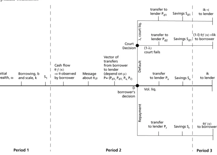
The timing of events is described in the timeline presented in figure 1. In the first period,
investors receive a bequest w. Then a borrowing contract defines an amount of borrowing b
and a scale of project, k. Finally borrowers save an amount s1. In the second period, the
borrower receive a cash flow and thus observes θ, issues a messageµ about the cashflow, and,
based on µ, a vector p is defined. Afterp is defined, the borrower takes the decision between
voluntarily liquidating, repaying or defaulting (decision node D). If the decision is default, the
court have a probability λ of liquidating and a probability (1−λ) of not liquidating. Notice
that in the second period, optimal savings are different for each branch of the three. I denote
savings under repayment, voluntary liquidation, default with liquidation and default without
liquidation respectively bysr, sv, sd1 andsd2.
When investors are taken to court but the court fails to liquidate, they have the possibility
to liquidate the project and obtain ik or wait for a cash flow. This is expressed by the binary
variable l, that takes value 1 if the decision is for liquidation and 0 if it is not to liquidate. A
proposition to be stated below shows that under reasonable conditions, borrowers will never
liquidate when courts fail to do so. This means that l will always be equal to zero in optimal
contracts. Therefore, throughout the paper, the term voluntary liquidation refers to liquidation
before investors are taken to courts. The inclusion of the possibility of voluntary liquidation
after courts - that could also be thought as another decision node after court decision in the
tree below - makes the model more realistic, and also helps in the derivation of properties of
optimal contracts.
Figure 1 - Timeline and Structure of the Problem
2.1
The Optimal Contract
Definition A borrowing contract is a triple {b, k, π(p, θ)}, where b ∈ B ⊆ < is the level of borrowing, k ∈ K ⊆ <+ is the scale of the project financed, and π : P ×Θ → (0,1) is the
joint probability distribution of p and θ.
Notice that savings in thefirst period,s1,are not part of the contract. In principle, contracts
could include s1 as a choice variable. If this were the case, the contract would need to produce
incentives for individuals to adopt the prescribed level of savings. But assuming that s1 is
equal to zero, and including in the contract incentives for people not to save positive amounts
rate, savings may be implicitly provided by the lender. Indeed, suppose a contract specifies
an amount of borrowing b, a saving amount of s1 and a distribution of p conditional on θ of
π(p|θ).With an alternative contract with borrowingseb=b−s1,and distribution of transfers
e
π(p+s1(i+r) | θ) = π(p | θ), and s1 = 0, consumers and the bank would face the same
resources in each state as in the first contract. Therefore, if they did not have incentives for
hidden savings in the first contract, they would not also have incentives for so in the new one.
Notice that this transformation may require a negative value of "borrowing ",eb. This is not
ruled out of the set of possible contracts. From now on, I assume thats1 = 0.But an incentive
constraint determining that no hidden savings (s1 >0) are desired by agents must be added to
the contract.
The solution to the problem is constructed backward. After transfers are given in the second
period, the borrower defines second period savings. Unlike in the first period, savings in the
second period may be bigger than zero, as there are no transfers between the borrower and
the lender in the third period. In the case of default and no liquidation by courts, individuals
also choose an optimal value of l, defining the decision between liquidating or not after being
released by courts. The second period savings decision and the choice of l determine indirect
utilities from the second period on conditional on transfers (that includes the utility from third
period). The indirect utilities in the second period under repayment, voluntary liquidation,
default with liquidation by courts and default without liquidation by courts are respectively
denoted by: Vr
2(θf(k), pr), V2v(θf(k), pv), V2d1(θf(k), pd1), and V2d2(θf(k), pd2). Notice that by
the concavity of U,all of these functions are concave on both arguments. I denote the indirect
utility under default as:
Vd
2(θf(k), pd1, pd2)≡V2d1(θf(k), pd1)λ+V2d2(θf(k), pd2)(1−λ).
At the decision node D, investors take the utility maximizing decision. Therefore, the
indirect utility in the second period given the vector pis:
V2(θf(k), p) = max{V2d(θf(k), pd1, pd2), V2v(θf(k), pv), V2r(θf(k), pr)}.
defined as follows:
d(θ, k, p) = 2 if V2v(θf(k), pv)> V2r(θf(k), pr) (1)
andV2v(θf(k), pv)≥V2d(θf(k), pd1, pd2)
d(θ, k, p) = 1 if V2r(θf(k), pr)≥max{V2d(θf(k), pd1, pd2), V2v(θf(k), pv)},
d(θ, k, p) = 0 if V2d(θf(k), pd1, pd2)>max{V2v(θf(k), pv), V2r(θf(k), pr)}
The functiondtakes value 1 when there is repayment, 2 when there is voluntary liquidation
and zero when there is default.
A first step in the characterization of the optimal contract is the definition of the optimal
distribution of transfers in the second period conditional on θ, when b , w and k are given.
The choice variable in this program isπ(θ, p),the joint probability distribution ofθ andp. The
choice of π(θ, p)is subject to the following conditions. First there is a technological constraint
stating that θ is distributed according to h(θ):
∀θ, X
p
π(p, θ) =h(θ). (2)
Second, the transfers policy must be such that investors have no incentives to hide cash flows:
∀θ,bθ < θ.
X
p
π(p|θ)V2(θf(k), p)≥
X
p
π(p|bθ)V2(θf(k), p). (3)
Another condition onπ is that individuals should have no incentive to make hidden savings. In
the case of risk neutrality this condition is innocuous. But if investors are risk averse, the effect
of savings on second period utilities depend onθ, pand the decision between repayment, default
and voluntary liquidation. With positive savings and risk aversion, (3) may not be a correct
characterization of incentives for individuals to report the truth cash flows. The condition for
∀µ:Θ→Θ with µ(θ)≤θ and∀ s1 ∈(0, b+w−k),
X
p,θ
π(p, θ)(U(B+w−k) +βV2(θf(k), p))≥ (4)
X
p,θ
π(p, µ(θ)) h(θ)
h(µ(θ))(U(B+w−k−s1) +βV2(θf(k), p+ (1 +r)s1)).
This condition states that for any reporting strategy,µ,there is no incentives to hidden savings.
The participation condition for the lender, or zero profit condition, is:
B(1 +r)≥X
p,θ
π(p, θ)[d(2−d)pr+
(1−d)(2−d)
2 (λ(pd2+
ik
1 +r) (5)
+(1−λ)pd1−c) + (d−1)
d
2(pv +
ik
1 +r)],
where d is defined by (1). The conditions forπ to be a probability distribution are:
π ≥0, X
p,θ
π(p, θ) = 1. (6)
Notice that given w, conditions (2) to (6) cannot be fulfilled for some values of k and b.
They can only defined for a set of feasible borrowing-scale combinations Γ(w). This is the set
of values ofk andbsuch that:
- (2) to (6)are valid for some π given w, b andk.
-b+w−k.≥0.
Clearly,Γ(w)is not empty. Indeed, setting k=w, b= 0, pd1 =pr =pv = 0,andpd2 =−ik,
all constraints of the problem are satisfied. This implies that at least one contract is available
to any individual.
Given w, for any (b, k) ∈ Γ(w), the optimal transfers in the second period are defined by
Program 1
e
V1(b, k, w) = max
π U(b+w−k) +β X
p,θ
π(p, θ)V2(θf(k), p), (7)
s.t. (2) to (6).
Given the function Ve1(b, k, w), it is possible to define the program determining the choices
of bandk given w andA. This program is:
Program 2 Ve(w) = max
(b,k)∈Γ(w)Ve1(b, k, w).
2.2
Some Properties of the Solution
This subsection presents some propositions describing the characteristics of optimal contracts.
These propositions depend basically on assumptions on the second period indirect utility
func-tions. Although these assumptions are stated in terms of the indirect utilities, they ultimately
depend on the function U. They are all valid for standard specifications of the utility function
U such asCARA and CRRA. Most of them (assumptions (a), (b), (c), (d) and (e)) are valid
with linear utility (risk neutrality). The assumptions used in the derivation of the results are:
Assumptions
(a)Vr
2(θf(k), p) is concave on pandθf(k).
(a’) Vr
2(θf(k), p)is strictly concave on p andθf(k).
(b) (∂2Vr
2(θf(k), p)/∂2p)/ (∂V2r(θf(k), p)/∂p) is nonincreasing with θf(k).
(c) −(∂2Vr
2(θf(k), p)/∂2p)/ (∂V2r(θf(k), p)/∂p) is nonincreasing with p.
(d) (∂2Vr
2(θf(k), p)/∂p∂θf(k))≥0.
(d’) (∂2Vr
2(θf(k), p)/∂p∂θf(k))>0.
(e) (∂2Vv
2(θf(k), p)/∂2p)/(∂V2v(θf(k), p)/∂p) is non increasing with θf(k).
Assumption (a) is a consequence ofU being concave. Condition (b) states that the absolute
with θ. Condition (c) that it is nonincreasing with transfers received in the second period.
Condition (d) states that the marginal utility of receiving transfers in the second period is
non-increasing withθ. Condition (e) states that the indirect utility of liquidators has nonicreasing
absolute risk aversion with respect to transfers in the second period. An absolute risk aversion
that is not increasing withθguarantees that if repayment or liquidation is certain, it is possible
to substitute lotteries for nonrandom utility equivalents without producing additional incentives
for high θ individuals to misreport their cashflows. Nonincreasing absolute risk aversion with
transfers received in the second period guarantees that this can be done without additional
incentives for hidden savings.
The following proposition states that there is a pooling value of repayment for all types that
pay with certainty. This is what makes the optimal contracts similar to debt contracts.
Proposition 1 Let b, k and w be given. Suppose that pr can assume any value in <, that
Assumptions (a) to (d) are valid and that Θ is finite. Then, if an optimal contract implies
that types θ1 and θ2 chose repayment with probability one, there exists an optimal contract in
which both types repay the same amount pbr with probability 1. If (a’) and (d’) are valid, this is
a necessary result: an optimal contract where types θ1 and θ2 repay with certainty must have
both types repaying the same amount with certainty.
Proof. See appendix 1
This follows from asymmetric information about cash flows. Ideally, with risk aversion, it
would be desirable to extract higher payments from individuals with high cashflows. But this
is not possible when cash flows can be hidden. Individuals with high cash flow realizations
would have incentives to misreport their cash flows. Therefore, the amount of repayment that
guarantees zero probability of project liquidation does not depend on θ. This bunching value
of repayments can be used to define borrowing interest rates as:
rb = b
pr
b −1, (8)
bor-rowing interest rate differs from r, the outside market saving interest rate.
The presence of a unique value of repayment for types that repay with certainty is directly
related to the fact that sometimes randomization is optimal contracts. Randomization may be
used to separate high cash flows from medium cash flow investors. Proposition 1 implies that
for values ofθ such that the probability of repayment is 1, the amount repaid does not depend
onθ.Individuals with very high values forθ tend to repay with probability one in order not to
loose their future cash flows. But it is possible that some values ofθ are not so high to justify
repayment at this pooling value, but are high enough to make it worth that a discount is given
on some occasions so that there is no liquidation. But these discounts cannot be offered with
probability one: a probability of liquidation9 must be given as a threat for high θ individuals
not to pretend to be one of these intermediate types.
The following lemma determines that, in optimal contracts, defaulters do not liquidate when
courts fail to liquidate, or, putting it differently, that l in figure 1 is always equal to zero.
Lemma 2 Let b, k and w be given. Suppose assumption (e) is valid and c > 0. Then, the probability that in the optimal contract d= 0 (default) and l = 1 (defaulters liquidate after courts fail to liquidate) is zero.
Proof. See appendix 1
Lemma 3 is useful in the proof of the next proposition.
Proposition 3 Given the conditions of Lemma 2, both an increase in the reliability of
courts, λ and a decrease in the cost of courts, c do not decrease welfare.
Proof. See appendix 1
This happens because both an increase in λ and a decrease in c increase the set of feasible
payoffs. This proposition determines that both an increase in the reliability of courts, λ and a
decrease in the cost of courts,ccan be interpreted as institutional improvements. The following
9Setting a value ofp
rthat is so high that the choice for liquidation or default is always optimal is equivalent
proposition reveals that both asymmetric information and uncertainty about the outcome of
courts are essential for default to be a possibility in optimal contracts. Also, it reveals that
without asymmetric information, there is no inefficient liquidation of projects. Projects are
liquidated only when the cashflows they produce are lower than their liquidation value.
Proposition 4 If there is no asymmetric information (constraints (4) and (3) are not
required) and courts are costly (c >0), there is no default and voluntary liquidation happens if and only if ik > θf(k).Also, even if there is asymmetric information, if λ=1 and courts are costly, there is no default.
Proof. I prove both claims by contradiction.
First, suppose that there is no asymmetric information and, when θ = θ, there is a positive
probability of default with a pair of transfers(pd1, pd2).In the case where ik > θf(k),settingλ
(pd1−c) + (1−λ)pd2 as the transfers from the borrower to the lender with voluntary liquidation
would increase the borrowers utility keeping the lenders revenue. If ik≤θf(k), settingλ(pd1−
c) + (1−λ)pd2 as the repayment value (pr) would allow an increase in utility keeping revenues
unchanged. Notice that if there were asymmetric information, this last arrangement might give
incentives for higher cash flow individuals to misreport their cash flow and pretend to be type
θ, thus repaying a lower amount. So the argument above is only valid without asymmetric
information.
Second, suppose there is asymmetric information, λ = 1 andθ =θ, and there is a positive
probability of default with the amount of transferspd1 (pd2 is irrelevant since failure by courts
have probability zero). Replacing this by voluntary liquidation with transfers pd1 would keep
utility constant, and therefore not affect incentives. But revenues of the lender would increase
3
Linear Programming Solution
As the solution to the optimal contract may involve randomization of transfers between
bor-rowers and lenders, a reasonable approach to solve the problem numerically is the discretization
of the choice and state space and the solution by linear programming. This approach has the
disadvantage that it lacks some precision because of the discrete gridding, but it has the
ad-vantage of being general and allowing for randomization. The functional forms used in the
solutions were:
U(c) = c
1−σ −1
1−σ
and
f(k) =kα.
In order to compute optimal transfers for a given level of A, k, b andw, (program1) I used a
grid with 12 values for θ, 50 values for pr, 30 values for pv and 5 values for pd1. Five possible
values of s1 were used in constraint (4). The distribution of θ used in the computations is
expressed infigure 210:
0 0.5 1 1.5 2 2.5 3 3.5 4
0 0.05 0.1 0.15 0.2 0.25 0.3 0.35
Figure 2 - Distribution of the Shockθ.
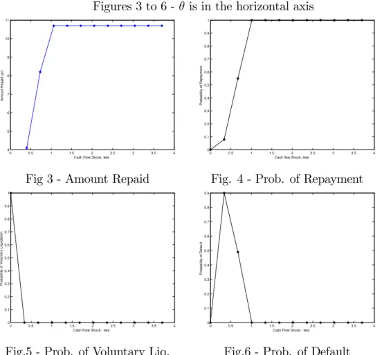
The following general features emerge from the solution of the Program 1, meaning that both
the amount of borrowing and the scale of projects are assumed to befixed. First, The repayment
schedule resembles a debt contract, in the sense that individuals with cashflows above a certain
level repay a common amount with certainty.
Borrowers with lower levels of cash flows may have a discount in the repayment value,
but they also have a positive probability of being assigned to liquidation or default. This
feature of the optimal contract is expressed in figures 3 and 4, computed for the following set
of parameters: c = 0.5, σ = 0.1, α = 0.5, i = 0.6, β = 0.95, r = 0.02, λ = 0.4, B = 9 and
k = 17. Figure 3 shows the amount repaid conditional on repayment, and figure 4 shows the
probability of repayment. These pictures provide an example in which randomization is used
in optimal contracts.
Figures 3 to 6 - θ is in the horizontal axis
0 0.5 1 1.5 2 2.5 3 3.5 4
4 5 6 7 8 9 10 11
Cash Flow Shock, teta
A m o u n t R e p a id ( p r)
Fig 3 - Amount Repaid
0 0.5 1 1.5 2 2.5 3 3.5 4
0 0.1 0.2 0.3 0.4 0.5 0.6 0.7 0.8 0.9 1
Cash flow Shock, teta
P ro b a b ili ty o f R e p a y m e n t
Fig. 4 - Prob. of Repayment
0 0.5 1 1.5 2 2.5 3 3.5 4
0 0.1 0.2 0.3 0.4 0.5 0.6 0.7 0.8 0.9 1
Cash Flow Shock - teta
P ro b a b ili ty o f V o lu n ta ry L iq u id a ti o n
Fig.5 - Prob. of Voluntary Liq.
0 0.5 1 1.5 2 2.5 3 3.5 4
0 0.1 0.2 0.3 0.4 0.5 0.6 0.7 0.8 0.9
Cash Flow Shock - teta
P ro b a b ili ty o f D e fa u lt
Another feature that is present in the optimal contracts is expressed in figures 5 and 6.
Figure 5 shows the probability of voluntary liquidation for each realization of θ. Figure 6
shows the probability of default per value of θ. Notice that despite the fact that there is a
positive costc= 0.5 of activating courts, default happens with positive probability in optimal
contracts. Individuals with high cash flows tend to be repayers. Individuals with very low
cashflows tend to voluntarily liquidate. Those with a intermediary levels of cash flows have a
positive probability of default. This pattern is observed in all numerical solutions obtained.
0 0.5 1 1.5 2 2.5 3 3.5 4 4.5 6
8 10 12 14 16 18 20
Relative Risk Aversion Coef. Minimal Transfer to Liquidators
Probability of repayment X 10 Repayment For High Cash Flows
Figure - 7
Another feature that is present in the solution of program 1, is that when borrowers
are risk averse, voluntary liquidators normally receive significant positive transfers from the
lender. These positive transfers work as an insurance device. Voluntary liquidators tend to be
individuals with low cashflows. Positive transfers to these individuals provide some level of risk
sharing. In the simulations, both the amount received by voluntary liquidators and the amount
paid by successful projects tend to increase with risk aversion. The amount paid by successful
investors reflects not only repayment of initial borrowing, but also payments to compensate the
transfers received in the contingency of low cashflows. Figure 7, shows, for the parameters used
amount of transfers received by voluntary liquidators and the probability of repayment evolve
with risk aversion. Notice that the fact that the probability of repayment decreases with risk
aversion also contributes for the values of repayments to be increasing with risk aversion.
4
Risk Neutrality and Continuum of Shocks
The solution with linear programming has the advantage that it is precise, admits lotteries
and allows the computation of the general model. However, especially with a fine grid of θ,
the curse of dimensionality becomes a serious problem, and solutions demand large amounts of
time and computational capacity. At this section, I specialize the analysis to risk neutrality,
with U(x) = x. For expositional convenience, I assume, without loss of generality, that β =
(1 +r) = 1. Imposing risk neutrality greatly simplifies the analysis. First, constraint (4) is not necessary: hidden savings does not provide any advantage to mitigate incentives, since it
contributes equally to utility in all branches of the tree in figure 1. Numerical solutions of the
model with risk neutrality show that, as the number of elements in the grid of possible values ofθ
increases, the fraction of points in which there is randomization tends to vanish. In other words,
as the support of θ approaches a continuum, the solution seems to converge to one in which
there is no randomization. So, I solve the problem assuming that there is no randomization
when there is a continuum ofθ and risk neutrality11.For this case, the characterization of the
solution is considerably simple, and is provided by proposition 5:
Proposition 5 Suppose borrowers are risk neutral, with utility given by U(x) = x, and
β = (1 +r) = 1,and no randomization conditional on θ is allowed. Then, there exists some optimal contracts with the following properties:
a- There exists a repayment value p such that whenever λθf(k)> p, or θ > θ3(p)≡p/λθf(k),
there is repayment of an amount p.
b- Whenever ik > θf(k), or θ < θ1 ≡ ik/f(k), there is voluntary liquidation, and pv =
−(1−λ)ik.
c- Whenever θ1 < θ < min(θ2, θ3), where θ2 ≡ (ik+ 1−λc )/f(k), there is voluntary liquidation
with and pv =−(1−λ)ik.
d-Whenever θ2 < θ < θ3,there is default with probability 1, withpd1 =pd2 = 0.
Proof. See Appendix 1.
Proposition 5 determines that whenever there is voluntary liquidation or default, the utility
of the borrower is equal to the utility of default with zero transfers. This utility is generated
by the values of pd1, pd2 and pv determined in proposition 5. Risk neutrality is essential for
that: there is no gains in making transfers to individuals with low cash flows, unless these
transfers are needed to rule out that the outside option of default is chosen. Higher transfers
from the lender to the borrower in the case of default and voluntary liquidation require higher
transfers from repayers. But higher repayment amounts may imply that a lower fraction of
cashflow realizations will justify repayment, and thus increase the probability that projects are
liquidated by value lower than their cash flow. Since the utility of defaulters and liquidators
is always equal to the utility of default with zero transfers, the decision between default and
voluntary liquidation depends on the revenue that is obtained with default and pd1 =pd2 = 0
and voluntary liquidation with pv =−(1−λ)ik. Notice from itemc of proposition 5 that asλ
tends to 1, the probability of default converges to zero, as stated in proposition 4.
From the properties presented in proposition 5, the characterization of the optimal contract
is straightforward. We characterize it for a continuum of θ, which can be interpreted as an
The repayment amount for individuals that repay, conditional on the size of loans, b and
the scale of project,k is such that the expected second period revenue of the borrower is equal
to the amount of borrowing in thefirst period. Therefore,p must solve:
b = λikH(θ1) +
Z min(θ2,θ3(p))
θ1
(ik−(1−λ)θf(k))h(θ)dθ (9)
+»(θ2 < θ3(p))
Z θ3(p)
θ2
(λik−c)h(θ)dθ+ (1−H(θ3(p))p
where » (θ2 < θ3(p)) is an indicator function that has value 1 when θ2 < θ3(p) and zero
otherwise. The right hand side of equation (9) is the revenue from the borrower given repayment
amount p. The determination of amount of repayment, p, given the amount borrowed, can be
seen in figure 312:
0 2 4 6 8 10
0 0.2 0.4 0.6 0.8 1 1.2 1.4
Repayment Amount by Repayers Revenue Borrowing Amount
Figure 8
The vertical line shows the value of pdetermined by (9). Notice that there is another higher
value of p that solves (9), but this implies a higher probability of liquidation of good projects
so it produces a lower utility for the borrower. The choice of pwill always be the smaller value
that satisfies (9).
12This was generated withk= 1, b= 0.8, i= 0.5, c= 0.2, λ = 0.7, θhas lognormal distribution withµ= 1 andσ= 1 andf(k) =k0.5
The utility conditional on borrowing and amount of capital is given by:
U(k, b) = (w−k+b) +f(k)E(θ) + (1−λ)ik(H(θ1)) + (10)
+
Z θ3(p(k,b))
θ1
(1−λ)θf(k)h(θ)dθ+
Z ∞
θ3(p(k,b))
(θf(k)−p(k, b))dθ.
The problem specialized for the risk neutral case with β = (1+r) = 1 and no randomization
becomes:
max
(k,b) U(k, b) (11)
s.t.w−k+b≥0and (3).
The constraint w−k+b ≥ 0 will always hold with equality when b >0. Indeed, if there
savings, diminishing the amount of borrowing and keeping capital constant will not decrease
utility. It will reduce the amount to be paid and thus the states in which liquidation happen.
Therefore, givenw, bcan be written as the following function of capital:
b= max{0, k−w} (12)
Substituting (12) in (10) and using the value ofpimplicitly defined in (9) it is possible to obtain
utility as a function of k given w.For the parametric specification used infigure 8, andw= 1,
the utility of the borrower as a function of the scale of the project is given by:
0.5 1 1.5 2 2.5 3 3.5 4 6
7 8 9 10 11 12 13 14
Scale of Project
B
o
rr
o
w
e
r'
s
U
ti
lit
y
The optimal scale of the project, the one that maximizes utility, is determined by the horizontal
line in figure 8.
The next proposition is consistent with the intuitive idea that better enforcement should
decrease the risk of no repayment and thus decrease interest rates.
Proposition 6 In the solution given by equations (9) to (12) (that is the solution for the
case with risk neutrality, no randomization conditional on θ and θ defined in a continuum), if
projects have a fixed scale and b >0, borrowing interest rates are decreasing with the reliability of courts λ.
Proof. Define the ∆(λ, p) as the right hand side of (9). Since scale is fixed, band k are both
fixed. Therefore, ∂rb
∂λ = −
1
b
∂∆(λ,p)/∂λ
∂∆(λ,p)/∂p. It is clear from (9) that ∂∆(λ, p)/∂λ > 0. Also, it must
be the case that ∂∆(λ, p)/∂p > 0, otherwise a decrease in p would increase revenue without
decreasing utility, implying that pis not optimal. Therefore, ∂rb
∂λ <0.
Notice that an essential condition for this to be valid is that the scale of projects is fixed.
4.1
Numerical Results for the Risk Neutral Case
This section presents numerical solutions for the risk neutral version of the model just described.
The model is solved for two specifications of the production function,f(k).Thefirst specification
is f(k) = k0.5. Then I use a production function with a higher curvature. The comparison
between this two specification reveals that the curvature of the production function is a key
ingredient in the determination of the characteristics of the solution. For thefirst specification I
depart from a baseline specification wherec= 0.3, i= 0.5and the distribution ofθis lognormal
with parameters µ = 1.375 and σ = 0.5. I compute the solutions for several levels of initial
wealth andλ.I also check how the solution respond to different values ofcandiand for different
specifications of the distribution of θ,h(θ). The interest rates results presented in this sections
refer to the borrowing interest rates, as defined in (8).
amounts of borrowing in order to be able tofinance big projects. But the amount of borrowing
individuals are able to obtain is limited: for very large loans, the maximum revenue that can
be obtained by the lender after the first period is lower than the amount of borrowing. Figure
10 shows, for the baseline specification and λ = 0.7, the optimal scale of projects and the
maximum possible scale achievable by agents as a function of their initial wealth. Notice that
there is some credit rationing. The maximum scale available for low wealth individuals is lower
than optimal scale for individuals that have very high wealth and therefore are unconstrained in
their choice of scale. This is similar to Evans and Jovanovic (1989). But differently from them,
even for very low wealth agents, the optimal scale is lower them the maximal scale available.
0 5 10 15 20 25 30 35
0 10 20 30 40 50 60
Initial Wealth Maximal Scale X Optimal Scale
Maximal Scale Optimal Scale
Figure 10
Figure 12, in appendix 2, shows the wealth profile of optimal project scale, size of loans
(amount of borrowing), probabilities of default, repayment and voluntary liquidation, and
bor-rowing interest rates, as defined in equation (8). These profiles are shown for 4 different values
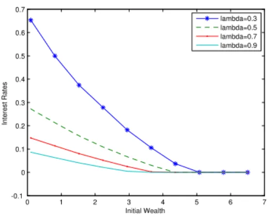
of the parameter of court reliability,λ:0.3, 0.5, 0.7 and 0.9. The results show that, for all levels
of λ investigated, the optimal scale of projects increase with the initial wealth, up to a point
where an optimal scale is achieved. The optimal size of loans profile has an inverted U shape:
it is increasing for very low levels of wealth, but after a some point it becomes decreasing. After
some level of wealth, individuals start to self finance their projects. Both the probability of
default and the interest rates are decreasing with initial wealth. Wealthier individuals not only
Notice that higher reliability of courts implies higher values of loans and capital. But the
effect of λ on interest rates and the probability of default is not clear. This is more evident in
figure 13, that shows, for 4 levels of initial wealth, the evolution of these same variables withλ.
Both the scale of projects and the size of loans (b) are increasing withλ, so the effectiveness of
legal enforcement increases scale of borrowing and projects. The effect of λ on the probability
of default and the borrowing interest rates is undetermined. For very high values of λ, the
probability of default is zero, as stated in proposition 4. But for very low levels ofλthe amount
of borrowing is extremely low, but these small borrowings have very low probabilities of default.
The intermediary values of λ are those that produce high probability of default. Interest rates
also have a non monotonic behavior. They tend to be low with very low levels of court reliability
and higher for intermediary levels of λ.
Another remarkable feature of figure 12 is that, as the initial wealth increase, the interest
rates and the probability of repayment both go down. This implies that interest rates are
not only determined by the probability of repayment. Notice that the as wealth increases, the
probability of voluntary liquidation also increase. When there is voluntary liquidation, the value
of liquidation is transferred to the lender or, putting it differently, there is collateral seizing by
the lender. More collateral transfers make it possible that the repayment generates a smaller
fraction of the lenders revenue after the first period. Figures 14 and 15, in appendix 2, show a
case in which there is no collateral value (i= 0). In this case, all revenue of the borrower comes
from repayment, and non repayment rates explain almost perfectly the interest rates profile.
Figures 19 and 20 in Appendix 2 show the numerical solutions for the optimal scale, interest
rates and the probability of default computed for alternative specifications forc, iandh13. Some
remarkable results from this analysis are that the probability of default and the interest rates
increase with the variance of θ, and decreases with the cost of courts c. Also, the scale of
projects tend to be higher as the liquidation value of projects increase.
The result that the interest rates may increase as the reliability of courts, λ, increases,
contrasts with proposition 6, valid for fixed scale. I recompute the problem using another
production function that has a higher curvature, and thus is closer to the case of fixed scale.
This production function is:
f(k) = (1 + (1−k)−2).
This is a CRRA function with a higher curvature than f(k) = k0.5 (or, in the utility context,
higher risk aversion) moved one unit to the left and summed by one so that it is always positive
and is zero valued atk = 0.Figure 11 plots both this production function (production function
2) and the one chosen before (production function 1). This new production function, with higher
curvature is closer to a fixed scale case. The gains of scale are initially high, but eventually
become very low.
0 1 2 3 4 5 6 7 8 9
0 0.5 1 1.5 2 2.5 3
Scale of Project
C
a
s
h
F
lo
w
Production Function 1 Production function 2
Figure 11
The baseline specification used in the analysis with this production function has c = 0.3,
i = 0.5 and the distribution of θ lognormal with parameters µ = 1.5 and σ = 0.375. The
solutions for a baseline case with this second specification are expressed infigures 16 and 17, in
of default decrease with wealth. Also, the scale of projects tend to increase both with wealth
andλ, although the variation on scale is proportionally smaller than in the first specification.
However, a remarkable difference that comes from this specification is that the probability
of repayment is tends to be increasing and interest rates are consistently decreasing with λ.
Better legal enforcement not only increases the scale of projects, but also decreases interest
rates. Further, both effects are higher for low wealth individuals. These numerical results,
combined with Proposition 6, indicate that the curvature of the production function is a key
ingredient to define how better enforcement affects interest rates.
Another ingredient that is affected by the curvature of the production function is the relation
between initial wealth and amount of borrowing. In the high curvature case (as well as in the
fixed scale case) the amount of borrowing is always decreasing with wealth. This differs from
the solution with low curvature, that has borrowing amounts initially increasing with wealth.
This is potentially useful for empirical work: the response of amount of borrowing to initial
wealth contains information about the curvature of the production function, and this curvature
is a key element to determine wether interest rates respond to quality of enforcement or not.
Figures 20 and 21 in Appendix 2 show the solutions for the optimal scale, interest rates
and the probability of default for this second production function and different specifications
fori, cand the distribution of θ, h(θ). The general features of the solution are similar to those
presented in Figure 16. A remarkable result, not present in the results for thefirst specification
of the production function is that, not only the interest rates are higher as the variance of θ
(risk of project) increases, but also the optimal scale of projects is significantly smaller.
5
Discussion and Concluding Remarks
This paper departs from a model that has debt contracts as optimal project financing
arrange-ments conditional on the environment. It is possible to define a borrowing interest rate from the
projects liquidated. This definition of borrowing interest rates can be used in an evaluation of
how interest rates and scale of projects respond jointly to the reliability of courts to enforce
contracts.
The results presented in the preceding sections can be divided in two cathegories, the
the-oretical findings and the numerical findings. On the theoretical side, two results can be
high-lighted. First, an increase in the reliability and a decrease in the cost of courts increase welfare.
Second, default may actually be observed in optimal contracts, but this requires both
asym-metric information and imperfect enforcement by courts. On the numerical side, there are four
main findings. First, wealthier individuals borrow with lower interest rates and run higher
scale enterprises. Second, The reliability of courts has a consistently positive effect on the scale
of projects. Third, the effect of bad enforcement on interest rates is undetermined when the
curvature of the production function is low, and it is negative when this curvature is high or
when projects have a fixed scale. Finally, the possibility of collateral seizing makes it possible
that interest rates and the probability of default have comovements.
The first theoretical finding has policy implications. The second theoretical finding shows
that asymmetric information generates the realistic feature that punishment may actually be
observed, which does not happen in most limited commitment models with perfect information
and in particular in this model, when asymmetric information is not present. The numerical
findings can be confronted with existing empirical work, and they may be used as a baseline
for further empirical investigation.
5.1
Evidence from empirical studies and empirical potential
Afirst result that is related with empirical studies is that the scale of projects increase with the
reliability of courts,λ. Higher scale of projects produce higher outputs, so the model generates
a theoretical link between development and the quality of institutions. This relation have been
explored in empirical studies such as Knack and Keefer(1995) and Mauro (1999) that present
and Acemoglu and Johnson (2005), that present evidence linking property rights institutions
and economic growth.
There is also an empirical literature that discusses the impact of institutions on the form offi
-nancial intermediation. This includes Acemoglu and Johnson (2005) and LaPortaet. al.(1998).
Examples of papers that explicitly relate the quality of judicial system and interest rates are
Leaven and Madjnoni (2003), that uses cross country data, and Costa and Mello (2006) and
Visaria (2005), both of which employ a natural experiment approach. These papers find
evi-dence that bad legal enforcement is connected with high interest rates. This is not generated by
all specifications of the model, but is consistent with the results from the second specification
of the production function, with high curvature.
Another prediction of the model that have support in empirical studies is that interest rates
are higher to low wealth individuals. Karlan and Ziemann (2006) report high interest rates in
loans for poor individuals in South Africa. This relation is also found by Araújo and Rodrigues
(2003), that use data from credit contracts recorded by the Brazilian Central Bank. They show
that the very high interest rates that are prevalent in Brazil affect most strongly small firms.
The average interest for firms that are classified by banks as micro-firms is 57%, for those that
are classified as small firms it is 44.78%, for medium size firms it is 33.66% and for big firms
it is 29.5%. In the model presented, in all parametrizations, wealthier individuals have lower
borrowing interest rates, so the model is consistent with these findings.
Another finding by Araújo and Rodrigues that is related with the results of the model is
that the average interest rates for large loans are smaller than that for big loans. Again, this
is not obtained in any specification of the model, but is consistent with at least two particular
cases. First, when the production function has low curvature, in the lower part of the wealth
distribution the size of loans increases and the interest rates decrease as the initial wealth
increases. If most of the credit contracts have borrowers in this lower part of the wealth
distribution, it is possible that higher loans have, on average, lower interest rates. Notice
high interest rates. Such specification is consistent with the Brazilian cross-sectional stylized
facts but do not to explain why interest rates in Brazil are higher than in most countries. A
second possible explanation for interest rates to be decreasing with size of loans comes from
difference in risk of projects. For the second specification of the production function, low
variance ofθ (or low risk on projects) generates simultaneously high scale of projects, and thus
large amounts of borrowing, and low interest rates (see Fig. 20, in appendix 2). The variability
on the risk of projects could generate a negative correlation between size of loans and interest
rates, and also help to explain the negative correlation between interest rates and scale offirms.
This second case departs from a specification of the production function that is consistent with
imperfect legal enforcement as an explanation for high interest rates.
An important result that comes from numerical analysis, is that the relation between wealth
and the amount of borrowing depends strongly on the curvature of the utility function.
There-fore, cross-sectional estimates on how the amount of borrowing relates to initial wealth could
provide some information about the curvature of the production function. This is important
since the curvature is a key ingredient to determine the effect of legal enforcement on interest
rates.
In order to evaluate how different specifications of the model fit real credit markets, it
is necessary to make a careful empirical analysis with adequate data. But the results just
presented illustrate that the model produces several testable implications, that could be useful
to confront the model with real credit markets. Also, with adequate data, further research could
define the specification of the model that better fit the data through structural estimation of
the model or an identifiable version of it. Estimates from different locations and periods, with
different legal environments could be compared. An estimated version of the model could also
5.2
Policy Implications
High interest rates and credit rationing, especially for poor individuals, are commonly regarded
as a problem in developing countries, and policies suggested to deal with them include subsidy
to credit, public provision of credit and interest rate controls. The model discussed presents
high interest rates and low amount of credits for low wealth individuals, but those are optimal
given the environment. If the model provides a good characterization of credit markets, such
policies would have no advantage over the mere redistribution of initial wealth. On the other
hand, proposition 3 and the fact that in simulations the contracts respond to the court quality
variables, indicate that improvements in legal enforcement could bring welfare gains. This
reinforces the importance of evaluating how well the model fits real credit markets data. A
research agenda in this direction could include a comparison of this model with other possible
explanations for high interest rates and low credit for poor individuals.
The negative result that interest rates may increase even with improvement in legal
enforce-ment also have consequences for policy evaluation. An increase in average interest rates does
not necessarily mean a welfare loss. Proposition 4 determines that increases in the reliability
of courts never produce welfare losses. However, sometimes interest rates increase with an
im-provement in enforcement. In those cases, the gain from the possibility of larger investments
more than compensates the losses that may come from higher interest rates. In principle, it is
possible that legal improvements expand the amount to credit and simultaneously produce an
increase in average interest rates. This may help to explain why countries like Brazil, that have
an intermediary level of development, have higher borrowing interest rates than less developed
and institutionally more unstable countries. In those countries, interest rates are lower, but the
amounts of formal borrowing are cosiderably smaller.
5.3
Theoretical extensions
The model employed is particularly simple in the dynamic structure. Repayment amounts are
by the fact that it affects only one cash flow. Therefore, an extension of the model, either
to more periods or infinite periods would certainly increase realism. Also, such an extension
could provide insights about the effect of legal enforcements on the term structure of borrowing
contracts.
Another possible theoretical extension would be to include ex-ante asymmetric information.
Individuals would have better information about their projects than the lender before borrowing
contracts are defined. Stiglitz and Weiss (1981) show that credit rationing can emerge in credit
markets as a result of adverse selection. But they receive criticism from Bester (1985) that shows
that collateral can be used to screen borrowers with different risks and overcome this problem.
It might be interesting to evaluate if the notion of collateral employed in the present paper
(scale of projects) would be able to produce such screening and, if so, under which conditions.
The current model takes the legal system as exogenous. But, in principle, it is possible to
make the parameters related to courts endogenous. One simple way to do so, would be to make
the reliability of courts an increasing function of amount invested in legal institutions. This
could possibly define the determinants of optimal investment on legal institutions, and serve as
6
References
Albuquerque, R. and Hopenhayn, H. (2004), "Optimal Lending Contracts and Firm Dynamics
". Review of Economic Studies, 77, pp. 285-315.
Aghion, Phillipe and Patrick Bolton (1996). "A Trickle-down Theory of Growth and
Devel-opment with Debt Overhang". Review of Economic Studies, 64, pp.151-172.
Bolton, P. and Sharfstein, D. (1990), ”A Theory of Predation Based on Agency Problems
in Financial Contracting”, American Economic Review, 80, 93-106.
Araújo, A. and Eduardo A. Rodrigues (2004),"Taxas de Juros Bancárias e Garantias Reais:
uma Avaliação Preliminar com Base nos Dados da Nova Central de Risco ", Central Bank of
Brazil, Mimeo.
Buera, F. (2006), "Persistency of Poverty, Financial Frictions and Entrepreneurship", mimeo,
Northwestern University.
Chang, C. (1990), ”The Dynamic Strucure of Optimal Debt Contracts”, Journal of Economic
Theory, 52, 68-86.
Costa, A.C. and Joao M.P. De Mello, (2006). "Judicial Risk and Credit Market Performance:
Micro Evidence from Brazilian Payroll Loans," NBER Working Papers 12252, National Bureau
of Economic Research, Inc.
DeMarzo, P. M. and M. J. Fishman (2003), ”Optimal Long-Term Financial Contracting
with Privetely Observed Cash Flows”, Mimeo.
Evans, David S. and Boyan Jovanovic. "An Estimated Model of Entrepreneurial Choice
Under Liquidity Constraints". Journal of Political Economy 97 (1989): 808 - 827.
Gale, D. and M. Hellwig (1985), ”Incentive Compatible Debt Contracts : The One Period
Greenwood, Jeremy and Boyan Jovanovic, "Financial Development, Growth, and the
Dis-tribution of Income," Journal of Political Economics v. 98 (1990), pp. 1076-1107.
Hart, O.(1995), "Firms, Contracts and Financial Structure", Oxford University Press.
Hart, O. and Moore, J. (1998), ”Default and Renegotiation: a Dynamic Model of Debt”,
Quarterly Journal of Economics, 113, 1-41.
Holtz-Eakin, Douglas, Joulfian, David and Harvey S. Rosen.(1994) “Sticking It Out:
En-trepreneurial Survival and Liquidity Constraints.” Journal of Political Economy 102: 53 - 75
.Karlan, D. and J. Zinman (2006), "Observing Unobservables: Identifying Information
Asymmetries with a Consumer Credit Field Experiment", mimeo, Yale University.
Krassa, S. and Anne Villamil (2000), ”Optimal Contracts When Enforcement is a Decision
Variable”, Econometrica, 68, 119-134.
Krasa, S., T. Sharma and A. Villamil (2004), ”Bankruptcy and Firm Finance”, University
of Illinois, Urbana-Champaign, Mimeo.
Laeven, L and Giovanni Madjnoni (2003), "Does Juditial Efficiency Lower the Cost of
Credit?", World Bank Policy Research Working Paper 3159.
La Porta, Rafael; Lopes-de-Silanes, F; Shleifer, A.; and Vishny, R. (1998), "Law and
Finance", Journal of Political Economy, 106(6), 1113-1155.
Lloyd-Ellis, Hew and Dan Bernhardtn , (2000) "Enterprise, Inequality, and Economic
De-velopment," Review of Economic Studies, v.67: 147-68.
Magnac, Thierry and Jean-Marc Robin, (1996)“Occupational Choice and Liquidity