FUNDAÇÃO GETULIO VARGAS
ESCOLA DE ECONOMIA DE SÃO PAULO
RICARDO MEDEIROS DOS SANTOS DA SILVA
IMPLIED HAZARD RATES ANALYSIS THROUGH
BRAZILIAN CORPORATE DEBT
SÃO PAULO
RICARDO MEDEIROS DOS SANTOS DA SILVA
IMPLIED HAZARD RATES ANALYSIS THROUGH
BRAZILIAN CORPORATE DEBT
Dissertação apresentada ao Programa de Mestrado Profissional da Escola de Economia de São Paulo, parte da Fundação Getulio Var-gas, como parte dos requisitos para a obtenção do título de Mestre em Economia, linha de Finanças Quantitativas.
Supervisor:
Prof. Dr. Alexandre de Oliveira
Silva, Ricardo Medeiros dos Santos da.
Implied Hazard Rates Analysis Through Brazilian Corporate Debt / Ricardo Medeiros dos Santos da Silva - 2015.
57f.
Orientador: Prof. Dr. Alexandre de Oliveira.
Dissertação (MPFE) - Escola de Economia de São Paulo.
1. Debêntures. 2. Títulos (Finanças). 3. Risco (Economia). 4. Swaps (Finanças). I. Oliveira, Alexandre. II. Dissertação (MPFE) - Escola de Economia de São Paulo. III. Título.
Agradecimentos
Ao amigo André Maialy, pelas valiosas contribuções, paciência e confiança deposi-tados nesta dissertação.
Aos meus colegas de sala, pelo companheirismo, ideias compartilhadas e o bom humor que me ajudaram a completar essa travessia.
À equipe da F3, pelo apoio incondicional nesta empreitada.
Ao meus amigos e família, pelo incentivo, torcida e compreensão que eventuais ausências são pouco perto de toda a vida que ainda compartilharemos juntos.
Ao João e ao Dudu, que ainda não entendem o que esse trabalho significa, mas a alegria que vocês me proporcionam serve de combustível para eu me superar. Espero poder retribuir ao longo da vida de vocês, mesmo que só como inspiração.
À minha mãe, Adelice, pelo amor incondicional e por encorajar a minha educação durante toda a vida, mesmo que seu "orgulho de mãe" seja o mesmo desde 1986. Ao meu pai, Sérgio, obrigado.
“Γν̟θι σαυτóν. M ηδ´ǫν αγαν´ .”
Resumo
No Brasil, o mercado de crédito corporativo ainda é sub-aproveitado. A maioria dos participantes não exploram e não operam no mercado secundário, especialmente no caso de debêntures. Apesar disso, há inúmeras ferramentas que poderiam ajudar os participantes do mercado a analisar o risco de crédito e encorajá-los a operar esses riscos no mercado secundário. Essa dissertação introduz um modelo livre de arbitragem que extrai a Perda Esperada Neutra ao Risco Implícita nos preços de mercado. É uma forma reduzida do modelo proposto por Duffie and Singleton(1999) e modela a estrutura a termo das taxas de juros através de uma Função Constante por Partes. Através do modelo, foi possível analisar a Curva de Perda Esperada Neutra ao Risco Implícita através dos diferentes instrumentos de emissores corporativos brasileiros, utilizando Títulos de Dívida, Swaps de Crédito e Debêntures. Foi possível comparar as diferentes curvas e decidir, em cada caso analisado, qual a melhor alternativa para se tomar o risco de crédito da empresa, via Títulos de Dívida, Debêntures ou Swaps de Crédito.
Abstract
The Brazilian corporate debt market is mostly underdeveloped. Most of the participants do not explore and trade in the secondary market, which is specially the case for debentures. In spite of this fact, there are a myriad of tools that could help market participants analyze credit risk, which could make them more willing to trade these risks in the secondary market. This dissertation provides an arbitrage-free model that extracts the implied Risk-Neutral Mean Loss Rates from market prices. It is a reduced form version of the model proposed by Duffie and Singleton (1999) and defines the term-structure of interest rates as a Piece-Wise Constant Function. Through this model, we were able to analyze the implied Risk-Neutral Mean Loss curve through different instruments of Brazilian corporate issuers, using bonds, CDS and debentures. We were able to compare the different curves and decide, in each case analyzed, which of them are best to take on the company’s credit risk, via bonds, CDS or debentures.
List of Figures
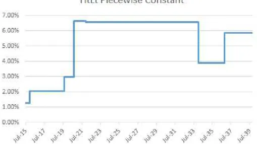
Figure 1 – HtLt Piece-Wise Constant from Vale Corporate Bonds in USD. . . 35
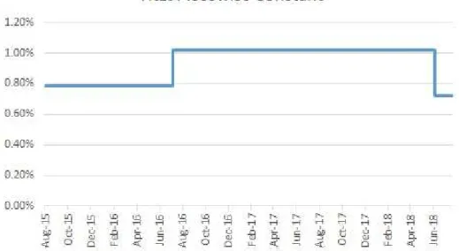
Figure 2 – HtLt Piece-Wise Constant from Vale CDS Spreads in USD. . . 36
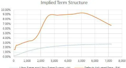
Figure 3 – Implied Term-Structure of Interest Rates from Vale Corporate Bonds in USD. . . 36
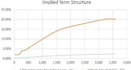
Figure 4 – Implied Term-Structure of Interest Rates from Vale CDS Spreads in USD. 37
Figure 5 – Cumulative HtLt from Vale Corporate Bonds in USD. . . 38
Figure 6 – Cumulative HtLt from Vale CDS Spreads in USD. . . 38
Figure 7 – HtLt Piece-Wise Constant from LRNE (DI+Spread) Debentures in BRL. 40
Figure 8 – HtLt Piece-Wise Constant from LRNE (IPCA+Spread) Debentures in BRL. . . 41
Figure 9 – Implied Term-Structure of Interest Rates from LRNE (DI+Spread) Debentures in BRL. . . 41
Figure 10 – Implied Term-Structure of Interest Rates from LRNE (IPCA+Spread) Debentures in BRL. . . 42
Figure 11 – Cumulative HtLt from LRNE (DI+Spread) Debentures in BRL. . . 42
Figure 12 – Cumulative HtLt from LRNE (IPCA+Spread) Debentures in BRL. . . 43
Figure 13 – HtLt Piece-Wise Constant from JSML (DI+Spread) Debentures in BRL. 44
Figure 14 – HtLt Piece-Wise Constant from JSML (%DI) Debentures in BRL. . . . 44
Figure 15 – HtLt Piece-Wise Constant from JSML (IPCA+Spread) Debentures in BRL. . . 45
Figure 16 – Implied Term-Structure of Interest Rates from JSML (DI+Spread) Debentures in BRL. . . 45
Figure 17 – Implied Term-Structure of Interest Rates from JSML (%DI) Debentures in BRL. . . 46
Figure 18 – Implied Term-Structure of Interest Rates from JSML (IPCA+Spread) Debentures in BRL. . . 46
Figure 19 – Cumulative HtLt from JSML (DI+Spread) Debentures in BRL. . . 47
Figure 20 – Cumulative HtLt from JSML (%DI) Debentures in BRL. . . 47
Figure 21 – Cumulative HtLt from JSML (IPCA+Spread) Debentures in BRL. . . 48
Figure 22 – HtLt Piece-Wise Constant from Vale (IPCA+Spread) Debentures in BRL (22.5% Tax-Discount). . . 49
Figure 23 – HtLt Piece-Wise Constant from Vale (IPCA+Spread) Debentures in BRL (15.0% Tax-Discount). . . 50
Figure 25 – Implied Term-Structure of Interest Rates from VALE (IPCA+Spread) Debentures in BRL (15.0% Tax-Discount). . . 51
Figure 26 – Cumulative HtLt from VALE (IPCA+Spread) Debentures in BRL (22.5% Tax-Discount). . . 51
List of Tables
Table 1 – Senior Unsecured Bonds - Issuer Information . . . 30
Table 2 – Libor Rates & Swaps in July 21, 2015.
Source: Bloomberg Terminal. . . 31
Table 3 – DI1 Futures Curve traded at BM&F Bovespa in August 10, 2015.
Source: Bloomberg Terminal. . . 32
Table 4 – Bootstrapped NTN-B Rates in August 10, 2015.
Source: ANBIMA. . . 32
Table 5 – Vale Corporate Bonds Prices in July 21, 2015.
Source: Bloomberg Terminal. . . 33
Table 6 – Vale CDS Spreads Curve in July 21, 2015.
Source: Bloomberg Terminal. . . 33
Table 7 – Debentures Prices (DI+Spread) in August 10, 2015.
Source: ANBIMA. . . 34
Table 8 – Debentures Prices (%DI) in August 10, 2015.
Source: ANBIMA. . . 34
Table 9 – Debentures Prices (IPCA+Spread) in August 10, 2015.
List of abbreviations and acronyms
ANBIMA Associação Brasileira das Entidades dos Mercados Financeiro e de Capitais
BM&F BOVESPA Bolsa de Valores, Mercadorias & Futuros de São Paulo
BRL Brazilian Real
CDI Certificado de Depósito Interbancário
CDO Collateralized Debt Obligation
CDS Credit Default Swap
CETIP Central de Custódia e de Liquidação Financeira de Títulos
CIR (COX; INGERSOLL; ROSS, 1985) CPI Consumer Price Index
IPCA Índice Nacional de Preços ao Consumidor Amplo
IRR Internal Rate of Return
LIBOR London Interbank Offer Rate
NTN-B Nota do Tesouro Nacional Série B
RFV Recovery of Face Value
RMV Recovery of Market Value
SIFMA Securities Industry and Financial Markets Association
USD US Dollar
Contents
I Introduction
15
1 Introduction . . . 16
1.1 Context . . . 16
1.2 Structure . . . 17
2 Literature Review . . . 18
2.1 Previous Work . . . 18
2.2 This Work . . . 20
II The Model
21
3 The Model . . . 223.1 Problem Statement . . . 22
3.2 Approach . . . 23
3.3 The Piece-Wise Constant Model . . . 25
3.3.1 Assumptions. . . 26
3.4 Estimation Process . . . 27
3.4.1 Bonds & Debentures . . . 27
3.4.2 Credit Default Swap (CDS) . . . 27
4 Model Application . . . 29
4.1 Scope . . . 29
4.2 Database. . . 30
4.2.1 Default-Free Interest Rate Curve . . . 31
4.2.2 Market Prices . . . 33
4.3 Application . . . 35
4.3.1 Vale USD Bonds and Vale CDS Spreads - July 21, 2015 . . . 35
5 Empirical Results . . . 40
5.1 Presentation . . . 40
5.2 Cross-Instruments Analysis . . . 40
5.2.1 LRNE DI+Spread and IPCA+Spread Debentures in BRL - August 10, 2015 . . . 40
5.2.2 JSML DI+Spread, %DI and IPCA+Spread Debentures in BRL -August 10, 2015 . . . 43
5.3 Tax-Exempt Debentures Analysis . . . 49
III Final Remarks
53
6 Conclusion . . . 54
7 Future Work . . . 55
Part I
16
1 Introduction
1.1 Context
Worldwide, the bond market has largely been used as long-term funding provider for public and private expenditures. When we talk about Corporate Debt only, it accounts for nearly 20% of the outstanding U.S. bond Market and has an average daily trading volume of 20 billion dollars.1 On the other hand, the locally traded Brazilian corporate
debentures market is much smaller, with an average trading volume of R$0.2 billion, but it has been growing since 2007. In 2014, the total volume of the Brazilian secondary market was around R$45 billion.2 It is reasonable to assume that the increase in trading volume is
due to a growing number of companies issuing new debt in the public market as well that the market participants are willing to assume that kind of risk. For market participants we include: portfolio managers, institutional investors, financial institutions and private investors.
Despite the fact that the majority of institutional investors do not trade in the secondary market, maybe for a lack of willingness or opportunity, there is a demand from the other participants to see more trades in the secondary market. In this context, the use and introduction of new tools to monitor credit risk is imperative to help market participants to price bonds, improve their analysis of new debt issues by a listed company or to even find, and explore, "distortions" in different bonds of a same issuer.
One way of approaching this matter is a model which could translate securities prices into a new measure that would serve as an alternative to analyze the issuer’s ability of repayment through different instruments. The main goal is to decide which of them is the best choice, if we are willing to take on the company’s credit risk.
In this work, we use the reduced-form model as proposed byDuffie and Singleton
(1999) to obtain the implied "Risk-Neutral Mean Loss Rate", HtLt, that compounds the
company’s hazard rate Ht (its implied probability of default) and its fractional lossLt, in
case of a default by the company. Using this measure, we will analyze Brazilian Corporate Debt through bonds, debentures and credit default swaps, looking for distortions that could make debt-owners more inclined to trade these securities in the secondary market.
1
According to the SIFMA Reports - http://www.sifma.org/research/statistics.aspx - July 21, 2015.
2
Chapter 1. Introduction 17
For companies that have bonds and a CDS Spread Curve, we have extracted the Risk-Neutral Mean Loss Rates from each instrument and confront them to search which of them is the best choice to take on the company’s credit risk; There is a special case in Brazil on which individual investors do not pay income tax investing in some debentures. We analyzed the Risk-Neutral Mean Loss Rates of a company in this special case and confront this curve with the other issues.
1.2 Structure
In Chapter 2, we present the Literature Review on the subject.
In Chapter 3, we will give a brief description of the Problem Statement in Section
3.1. The mathematical approach of Duffie and Singleton (1999) is in Section 3.2 and we detail the proposed Piece-Wise Constant Model by Meres and Almeida(2008) in Section
3.3. The Estimation Process that guarantees the arbitrage-free condition is presented in Section 3.4.
Chapter 4will show the scope of the applied problem (Section 4.1), the Database is presented in Section 4.2 and the Application in Section4.3.
18
2 Literature Review
2.1 Previous Work
The structural model of Merton (1974) is the first work introducing probability of default, where he proposed that the value a corporate bond is a function of three factors: risk-free interest rate rt; the specifications of the corporate bond indenture (like
maturity date, coupon rate, seniority, etc.); and the probability of default, when the firm is unable to satisfy some (or all) of the bond’s requirements. He estimated the latter based on the firm’s balance sheet, comparing the volatility of the company’s assets to its debts to estimate the risk of default. The model uses risky discount bonds to infer a risk structure of interest rates and analyze callable and coupon bonds. Even though the structural models are more economically intuitive, the periodicity of the balance sheets, which contain information about the asset or his liability structure, results in a set of imperfect information. Additionally, in cases of fraud, the balance sheets could not reflect the real economical situation of the company. These practical limitations could make a structural model become a reduced-form model, as showed in Duffie and Lando (2001). This and other types of structural models are beyond the scope of this work.
The reduced-form model of Litterman and Iben (1991) defines that a corporate bond depends on three components as well: the term structure of Treasury interest rates, embedded option values (in callable bonds) and the credit risk. They confront the usual way of a constant credit spread over the Treasury curve, arguing that it should account for (and increase with) the maturity of the bond. Their work use defaultable bonds in a discrete time model with zero recovery, proposing that the risky interest rate could be represented by an adjusted short-term rate. Their important result is that the corporate spreads over the Treasury are generally upward slopping, indicating that the market requires a higher risk premium to carry long-term bonds, therefore implying an increasing probability of default. This result makes a significant difference when pricing the embedded option on callable bonds.
Duffie and Singleton (1999) present the type of reduced-form model and this type used in this work. They assume an arbitrage-free setting to propose a discrete time model for defaultable bonds that extract the "risk-neutral mean-loss rate", HtLt, of
the instrument due to default. The bond is discounted by an adjusted short rate that accounts for probability of default and the fractional loss on default. There’s an important assumption that the process hL is exogenous, i.e. it does not depend on the value of the
Chapter 2. Literature Review 19
market value after the event of default, as if the event has not occurred. They showed that is not possible to identify separatelyHt andLtfrom corporate bond prices. One limitation
of models that use an adjusted short-term rate is that they cannot deal with jumps in interest rates. Specifically, this model assumes that the defaultable claim does not have a "jump" in its price at default time, which is a limitation. Most of the work on hazard rates
for Brazilian debt is based on this model, including this one.
The general formula of Collin-Dufresne, Goldstein and Hugonnier (2004) is a continuous-time setting model applicable even when the no-jump condition is violated. In contrast with the previous reduced-form models, this model allow the risk-free interest rate to be affected by the default event. They investigate the pricing of defaultable bonds in three different scenarios: flight to quality,counterparty risk and the systematic jump risk. They define the probability measureP′ which is different from the risk-neutral probability Q. This probability measure puts zero mass on paths where default occurs prior to the
maturity, where the probability measure is not continuous relative to the risk-neutral probability measure. They claim that it attacks not only the no-jump condition but it considerably simplify the calculations. Accounting the counterparty risk, they were able to evaluate collateralized debt obligation (CDO) as well.
Meres and Almeida (2008) applied one modified version of Duffie and Singleton
(1999) to estimate probabilities of default in Brazilian Global Bonds. They modeled the hazard rates as a piece-wise constant function of time t with three parts (short-term,
medium-term and long-term) and compare their model with the market prices using Root Mean Square Errors (RMSE) on three different dates: August 10, 2001; September 27, 2002 and November 19, 2004; They also use it to price an "out-of-sample" bond and the results are important to show the ability of their model in pricing newly issued bonds, as they priced one out-of-sample Brazilian Global Bond with an error five times lower than a simple linear interpolation. Their piece-wise approach to estimate Brazilian global bonds term-structure of interest rates is a closed-formula, it is an arbitrage-free model, as in Sharef and Filipović (2004), a characteristic that is not common in most of parametric term structure models. Although they claim that the term structures of interest rates have their movements primarily driven by three factors, which would backup their choice of using only three parts in the piece-wise constant function, it prevents the model from fitting perfectly with the market prices. Additionally, they used a fixed fractional L= 0.5.
Chapter 2. Literature Review 20
rates becomes a smooth curve, a function that has derivatives everywhere in its domain. The limitations of this work are the same of the previous one: fixed fractional loss in
L= 0.5 and only three parts in the composition of the hazard rates functions.
Most recently,Fernandez (2014) estimated hazard rates from Brazilian debentures grouped by their credit rating. The path chosen is to model the term-structure of interest rates as the parametric model proposed by Diebold and Li (2006), a modified version of
Nelson and Siegel (1987), and used the same discrete time model for defaultable bonds in
Duffie and Singleton (1999) to estimate hazard rates for a fixed fractional lossL= 0.8. To
study the consequences in hazard rates during a loose monetary policy cycle started by Brazilian Central Bank, he extracted the hazard rates for three different dates: February 29, 2012; August 31, 2012 and February 28, 2013. During this time, the implied hazard rates lowered as well. He argues that lower interest rates reduce the default risk of the companies, because they are able to issue more debt at a lower cost. Since he used a parametric model for the term-structure of interest rates, his model is not arbitrage-free, and, therefore, his term-structure does not reflect all the market prices at that time. That would be a limitation if you wanted to extract hazard rates as information to trade this debentures, as you could see arbitrage opportunities where there are none indeed.
In their model,Duffie and Singleton(1999) assume that the security does not jump at the default time, even though it could have "surprise" jumps along its life prior to default, which is a limitation that does not hold for all defaultable claims. Collin-Dufresne, Goldstein and Hugonnier (2004) tried to circumvent this restriction and showed that their model performs well in scenarios in which this condition fails. Despite this fact, we choose to do this work based in the discrete-time setting proposed by Duffie and Singleton (1999) because we wanted a deeper understanding of how it was applied in previous studies with Brazilian Debt before we study scenarios with jumps on interest rates.
2.2 This Work
This work is based onDuffie and Singleton (1999) and we will try to extract the Risk-Neutral Mean Loss Rate, HtLt, for a same issuer through different instruments fitting
the market information. In order to achieve this goal, we will use a Piece-Wise Constant Model with N parts, proposed by Meres and Almeida (2008), whereN is the number of
bonds available for that issuer. When information is available, we will confront the implied
HtLt extracted from the bond prices with the one extracted from the company’s CDS
Part II
22
3 The Model
3.1 Problem Statement
The price of a defaultable claim is a function of the bond’s (or debenture’s1)
specifications and the yield required by the creditor to take on the issuer’s risk. The former is defined by the bond’s indentures:
• Maturity Date: the date when the bond will redeem the issue by paying the face
value (or principal).
• Coupon: the periodic interest payment made to owners during the life of the bond.
It could be a fixed rate (on the principal), inflation-indexed or a floating rate.
• Seniority: is the order (rank) of repayment in the event of default.
• Embedded Options: the bond could be callable (or putable) prior to the maturity date. When a bond is callable (putable) it gives the issuer (the creditor) the right to retire (to sell back) the debt at par value.
The latter is the yield required by the creditors to take on the debt. According toFabozzi and Mann (2012):
"The yield on any investment is computed by determining the interest rate that will make the present value of the cash flow from the investment equal to the price of the investment."
For corporate bonds, creditors should account for their proper default-free interest rate. In a risk-aversion scenario, there is no economical reason to lend money to a company that is subject to default without charging a premium above default-free interest rate. Mostly, the default-free interest rate curve is changed by government monetary policy and future market expectations. The company’s default risk is governed by market expectations on the company’s ability of repayment. Changes in both should be reflected in the rate required by the creditors to take on this debt, which is composed of the default-free plus a risk premium function of the company’s default risk. The main scope of this work is to separate these components and extract the default risk implied by market prices, assuming it as the only explanation variable.
1
Chapter 3. The Model 23
What are the components that should affect this yield2? How it should be
esti-mated for a new issue? This yield is observable from market prices (and vice versa) and, consequently, will change overtime according to the trades registered in the secondary market. What are the consequences of these changes on the company’s default risk? These are the questions that we try to clarify in this work.
One way to explain is to look at the company’s credit risk. There are different approaches in modeling credit risk, mostly in the way the information is recognized. When complete information is assumed, the structural models take place trying to estimate the probability of default. On the other hand, when the hypothesis of incomplete information is assumed, we can use reduced-form models to estimate the conditional probabilities of default3. In this work, we adopt the reduced form model of Duffie and Singleton(1999) to
extract the Risk-Neutral Mean Loss Rates implied by Market Prices, which is consistent with a scenario of incomplete information.
Consider a collection of bonds with different maturities from a same company, each one has their price and yield to maturity. With that information, we can compose its Term-Structure of Interest Rates. Although they still could have different coupon rates, we assume that they share a same Default-Free Interest Rate Curve by now. So, our objective is to examine the difference between the Term-Structure of Interest Rates from the bonds collection and the Default-Free Interest Rate Curve and how this difference could be translated in a curve that represents the company’s default risk.
3.2 Approach
This model approaches the default risk as an unpredictable event governed by a hazard-rate process, as proposed by Duffie and Singleton (1999) for a discrete-time setting.
Consider a defaultable contingent claim that promises to payXt+τ at its
maturity date t+τ. For any times ≥t, let be:
• Hs the conditional probability at time s under risk-neutral probability
measure Q of default betweens and s+ 1 given the information available
at time s.
• ϕs denote the recovery in units of account, in our case USD or BRL, in
the event of default at s.
• rs be the default-free short-term rate.
To ensure the absence of arbitrage in the market, it is necessary to assume that discounted prices of defaultable bonds are martingales under the risk neutral measure Q.
2
Also called the Internal Rate of Return (IRR) or Yield to Maturity (YTM).
3
Chapter 3. The Model 24
So, if the asset has not defaulted at timet, we can write the fair price of a defaultable
bond at time t as a function of its price at timet+ 1 composed by two terms: one paying
the discounted fair price at time t+ 1 in the event of no-default; the other paying the
recovery value ϕt+1 at the event of default happening between t and t+ 1:
Vt= (1−Ht)e−rtEtQ(Vt+1) +Hte−rtEtQ(ϕt+1) (3.1)
Looking forward the over the life of the bond, Duffie and Singleton apply a recursive method to show that Vt can be expressed as:
Vt=EtQ "τ−1
X
j=0
Ht+je −
Pj
k=0rt+k
ϕt+j+1
j Y
l=0
(1−Ht+l−1)
#
+EtQ "
e−
Pτ−1
k=0rt+k
Xt+τ τ Y
j=1
(1−Ht+j−1)
#
(3.2)
Since the evaluation of Equation 3.2is not trivial, there is a crucial observation to be made: under the event of default at time s+ 1, the risk-neutral expected recovery at
time s can be simplified to be a fraction 1−Ls of the bond’s market value at times+ 1,
where Ls is an adapted process bounded by 1 that represents the fractional loss. By these
terms, the "Recovery of Market Value" (RMV) is given by:
EsQ(ϕs+1) = (1−Ls)EsQ(Vs+1)
and then the Equation 3.2 is simplified to:
Vt= (1−Ht)e−rtE Q
t (Vt+1) +Hte−rt(1−Lt)E Q t (Vt+1)
=EtQ e −
Pτ−1
j=0Rt+j
Xt+τ !
(3.3)
with
e−Rt = (1−H
t)e−rt+Hte−rt(1−Lt) (3.4)
Note that, in Equation 3.3, the present value of the promised payoff Xt+τ is
expressed as if it were default-free, discounted by the default-adjusted rate Rt. If we take
small time periods and the rates are annualized, it can be seen that Rt≃rt+HtLt. In
this case, under the assumption that Ht andLt are anexogenous process4, instead of using
the usual short rate rt, we can use use this default-adjusted rate Rt= rt+HtLt as the
bond’s discount rate.
4
Chapter 3. The Model 25
Now that we have scaled down our problem to looking for the default-adjusted rate,
Duffie and Singleton (1999) discussed two approaches: one is to parametrize R directly
or parametrize the component process r and hL. Since the main goal of this work is to
extract hLfrom market prices, we will use the second approach. We will parametrize r
with the proper default-free yield curve that is applicable to that corporate bond market. Given that hL is the risk-neutral mean-loss rate of the instrument due to default, and for
non-callable bonds they cannot be identified separately, we will use bond prices prior to default to extract hL, even though we could not identify h and L independently. There
are some ways to attack this identification problem of Lt, but we will try to explore the
product hL from market prices in distinct situations. The result will be the risk-neutral
mean loss rate curve that fits the bond market prices for that company.
3.3 The Piece-Wise Constant Model
AlthoughMeres and Almeida (2008) proposed a piece-wise constant model for the hazard rates with a constant fractional loss rate, we will use the same model without assuming a value for Lt. By this approach, for an issuer we have that its risk-neutral mean
loss is given by:
HtLt= N X
j=1
✶{tj−1<t≤tj}{HjLj} (3.5)
where ✶ represents an indicator function5 and the risk-neutral mean loss rates H
1L1,
H2L2, . . . , HNLN are constants. Meres and Almeida (2008) argue that this function is
a particular hazard-rate process and results in an arbitrage-free model, according to the Theorem 1 in Duffie and Singleton (1999).
Instead of using an arbitrary way, like N = 3 (accounting for short-term,
medium-term andlong-term), we propose the use of all market data available for a this issuer to obtain N, the number of pieces in Equation (3.5). First, consider a company that has
issued only one bond: a zero-coupon with time to maturity T1 and $1.00 of face value.
Using equations (3.3) and (3.5), the bond price should be given by:
P1(t, t+T1) =EtQ e −
Pt+T1
j=t+1Rj !
=e−
Pt+T1
j=t+1HjLjEQ t e
−Pt+T1
j=t+1rj !
=e−H1L1(T1−t)Pdef aultf ree(t, t+T1) (3.6)
where Pdef aultf ree(t, t+T1) is the price of a default-free bond with the same maturity T1,
priced in time t.
Now consider that same company issued one more zero-coupon bond with maturity
T2 > T1, we will have:
5
Chapter 3. The Model 26
P2(t, t+T2) =EtQ e −
Pt+T2
j=t+1Rj !
=e−P
t+T2
j=t+1HjLjEQ t e
−Pt+T2
j=t+1rj !
=e−
H1L1(T1−t)+H2L2(T2−T1)
Pdef aultf ree(t, t+T2) (3.7)
At last, if a company has issued N zero-coupon bonds with maturities T1 < T2 < · · ·< TN, pricing the bond with maturity TN will result:
PN(t, t+TN) =EtQ e −
Pt+TN
j=t+1Rj !
=e−P
t+TN
j=t+1HjLjEQ t e
−Pt+TN
j=t+1rj !
=e−
PM
j=1HjLj(tj−tj−1)+HNLN(TN−tM)
Pdef aultf ree(t, t+TN) (3.8)
whereM is such that tM < TN.
Furthermore, the term structure of interest rates RT will be given by:
RT =rdef aultf ree(T) +
1
T
M X
j=1
HjLj(tj−tj−1) +HNLN(T −tM) !
(3.9)
whererdef aultf ree(T) is the default-free spot rate up to time T. Note that all rates
must be annualized.
3.3.1 Assumptions
One of the model’s assumptions ofDuffie and Singleton (1999) is that the security does not jump when the default arrives, which is a limitation. Another important issue is that, after the default, the recovery is at market value (RMV) of the bond and not at face value (RFV). They showed that the choice of recovery involves both conceptual and computational trade-offs. Although the RMV is easier to use, if one assumes liquidation at default when absolute priority applies, the RFV is more realistic because it implies equal recovery for bonds with the same seniority. Then, the authors decided to confront the pricing implications under the RMV and RFV for a multi-factor CIR6 as the term
structure of interest rates Rt, with constant fractional lossLt= Land results showed that
implied hazard rates were similar for both. Therefore, we assume the RMV has the benefit of being an easier model without result in a loss of precision for our choice of Rt.
In the model, for a company with only one bond (or debenture), the Risk-Neutral Mean Loss Rate, HtLt, is constant through the whole life of the bond. The careful reader
might argue that it should change overtime, specially for bonds with longer maturities,
6
Chapter 3. The Model 27
probably in an upward slopping curve. But, since we cannot strip the bond coupons across all markets, we will extract HtLt piece-wise constant subject to market data and as an
arbitrage-free model, i.e. it should perfectly fit with market prices. Furthermore, we have used "closing prices" in our estimations, which do not account for bid/offer spreads and which is the liquidity effect in each security.
3.4 Estimation Process
3.4.1 Bonds & Debentures
Suppose a collection of m bonds of an issuer that share the same characteristics:
currency, coupon calculation type (floating or fixed rate) and payment seniority. Currency and calculation type will provide information about therdef aultf ree curve and the latter will
give us information about the fractional loss Lt. Since we are extracting the risk-neutral
mean loss rate HtLt altogether, we will group the bonds with a sameLt (at least for now).
Assume the prices Pj,j = 1, . . . , m andCjk, j = 1, . . . , m;k = 1, . . . , γj as the cash flow k
of bond j that is paid in Tj,k. So we will extract HiLi, i= 1, . . . , mthat make:
Pj = γj
X
k=1
Cjke−Tj,kR(Tj,k) (3.10)
where R(.) is the default-adjusted interest rate given by Equation3.9.
Prior, we already defined that m, the number of pieces in Equation 3.9, would
be chosen by the collection of bonds, i.e. the information available on that issuer. The estimation process used in this work is a bootstrapping method7. The result will be the
risk-neutral mean loss rate curve, piece-wise constant, that fits market prices for a given issuer/company. Based on that curve, we will get the Cumulative Risk-Neutral Mean Loss Rate.
3.4.2 Credit Default Swap (CDS)
According to the model proposed by Caratori (2008), we can estimate the risk-neutral mean loss rates based on CDS Spreads Curve with m different maturities using
the equation:
7
Chapter 3. The Model 28
Mj
X
k=1
"hr
def aultf ree(Tj) + (SCDS(Tj)−CCDS(Tj))
1 + rdef aultf ree(Tj)
2
i
nj
e−R(tj,k)[t−tj,k]
#
+e−R(Tj)[Tj−t]= 1 (3.11) whereMj is the number of payments in the life of the (j−th) CDS, with maturityTj and
coupon frequency per year nj; rdef aultf ree(Tj) is the default-free spot rate up to time Tj;
SCDS(Tj) is the CDS spread with maturityTj andCCDS(Tj) is the CDS coupon rate;tj,k is
the time of payment of thek−th coupon of the j−th CDS;R(tj,k) is the default-adjusted
rate given by Equation 3.9. The term
1 +rdef aultf ree(Tj)
2
is a correction derived of CDS’ absence of protection on the accrual interest rate.8
8
29
4 Model Application
4.1 Scope
The sample is a set of Brazilian corporate bonds issued in USD and BRL. Debentures in BRL are subdivided by their respective coupon calculation type: %DI1, DI+Spread and
IPCA2+Spread. Each group has their proper Default-Free Interest Rate Curve. Since the
Piece-Wise Constant is a function of the total of bonds issued, the sample was defined by issuers with the larger number of bonds available.
First, we have modeled the cash flow for each bond according to its indentures. For bonds in USD, we have used the Cash Flow Analysis - CSHF function from a Bloomberg Terminal. For debentures, we have used the ANBIMA website3, DEBENTURES Website4
and checked with CETIP Calculator5. In the estimation process, we used the Goal Seek
Tool from Microsoft Excel to search for the Implied Risk-Neutral Mean Loss Rate HtLt,
from the short-term to the long-term maturities bonds, which made the prices in Equation
3.10 fit market data. In a similar way, we estimated the CDS directly using the Equation
3.11. Furthermore, we plotted the graphs withPiece-Wise Constant Function, with the
Implied Term-Structure of Interest Rates and with the Cumulative HtLt. The analysis is
divided into two groups:
• Cross-Instruments Analysis: for companies that have bonds and a CDS Spread Curve and/or debentures with different Default-Free Interest Rate Curve, we have extracted their Risk-Neutral Mean Loss Rates using these instruments, and confront them, aiming to find the best choice to take on the company’s credit risk.
• Tax-Exempt Analysis: In Brazil, there are tax-exempt debentures on which individual investors do not pay income tax. We analyzed the Risk-Neutral Mean Loss Rates of a company in this special case and confront this curve with the other issues.
1
DI-Cetip Overnight Rate - http://estatisticas.cetip.com.br/astec/di_documentos/metodologia1_i1.htm - July 21, 2015.
2
Brazilian CPI - http://www.ibge.gov.br/home/estatistica/indicadores/precos/inpc_ipca/defaultinpc.shtm - July 21, 2015.
3
Deliberação no
3 - http://portal.anbima.com.br/tesouraria/regulacao/codigo-de-negociacao-de-instrumentos-financeiros/Documents/Deliberacao_n03.pdf - August 10, 2015.
4
http://www.debentures.com.br/exploreosnd/consultaadados/emissoesdedebentures/caracteristicas_f.asp - in August 10, 2015.
5
Chapter 4. Model Application 30
Additionally, in Section4.3, we have detailed one case of the Cross-Instruments Analysis, where we confront Vale corporate bonds and Vale CDS Spreads. The other analyses are done in the same way and they are presented in Chapter 5.
4.2 Database
Data used in this work is compiled by issuer, currency, coupon calculation type and payment seniority6, showed in Table 1.
Ticker Issuer Maturity Cpn. Calc. Type Currency Coupon
JSML15 JSL S/A 24-May-16 DI+Spread BRL 1.85% JSML16 JSL S/A 15-Jul-18 DI+Spread BRL 1.80% JSML18 JSL S/A 15-Jun-19 %DI BRL 116.00% JSML26 JSL S/A 15-Jul-20 DI+Spread BRL 2.20% JSML28 JSL S/A 15-Jun-21 IPCA+Spread BRL 8.00% JSML36 JSL S/A 15-Jul-20 IPCA+Spread BRL 7.50% JSML38 JSL S/A 15-Jun-21 %DI BRL 118.50% LRNE14 Lojas Renner S/A 15-Jul-16 DI+Spread BRL 1.10% LRNE15 Lojas Renner S/A 15-Jun-18 DI+Spread BRL 0.97% LRNE16 Lojas Renner S/A 01-Aug-18 DI+Spread BRL 0.85% LRNE24 Lojas Renner S/A 15-Jul-17 IPCA+Spread BRL 7.80% LRNE25 Lojas Renner S/A 15-Jun-19 IPCA+Spread BRL 5.70% VALEBZ Vale Overseas Ltd 11-Jan-16 Fixed USD 6.25% VALEBZ Vale Overseas Ltd 23-Jan-17 Fixed USD 6.25% VALEBZ Vale Overseas Ltd 15-Sep-19 Fixed USD 5.63% VALEBZ Vale Overseas Ltd 15-Sep-20 Fixed USD 4.63% VALEBZ Vale Overseas Ltd 11-Jan-22 Fixed USD 4.38% VALEBZ Vale Overseas Ltd 17-Jan-34 Fixed USD 8.25% VALEBZ Vale Overseas Ltd 21-Nov-36 Fixed USD 6.88% VALEBZ Vale Overseas Ltd 10-Nov-39 Fixed USD 6.88% VALEE18 Vale S/A 15-Jan-21 IPCA+Spread BRL 6.46% VALEE28 Vale S/A 15-Jan-24 IPCA+Spread BRL 6.57% VALEE38 Vale S/A 15-Jan-26 IPCA+Spread BRL 6.71% VALEE48 Vale S/A 15-Jan-29 IPCA+Spread BRL 6.78%
Table 1 – Senior Unsecured Bonds - Issuer Information
6
Chapter 4. Model Application 31
4.2.1 Default-Free Interest Rate Curve
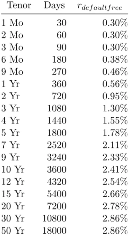
• Bonds and CDS (USD): Libor Rates and Libor Rates Swaps bootstrapped into a Theoretical Spot Rate Curve, as showed in Table2.
Tenor Days rdef aultf ree
1 Mo 30 0.30%
2 Mo 60 0.30%
3 Mo 90 0.30%
6 Mo 180 0.38% 9 Mo 270 0.46% 1 Yr 360 0.56% 2 Yr 720 0.95% 3 Yr 1080 1.30% 4 Yr 1440 1.55% 5 Yr 1800 1.78% 7 Yr 2520 2.11% 9 Yr 3240 2.33% 10 Yr 3600 2.41% 12 Yr 4320 2.54% 15 Yr 5400 2.66% 20 Yr 7200 2.78% 30 Yr 10800 2.86% 50 Yr 18000 2.86%
Table 2 – Libor Rates & Swaps in July 21, 2015. Source: Bloomberg Terminal.
• DI-Linked debentures (BRL): DI1 Futures Curve traded at BM&F Bovespa7,
as showed in Table 3.
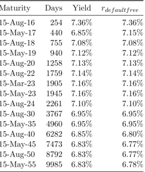
• IPCA-Linked debentures (BRL):Brazilian IPCA-Linked sovereign bonds (NTN-B8) yields bootstrapped into a Theoretical Spot Rate Curve, as showed in Table
4.
7
DI1 Futures - http://www.bmfbovespa.com.br/shared/iframe.aspx?altura=1300&idioma=pt-br&url=www.bmf.com.br/bmfbovespa/pages/contratos1/contratosProdutosFinanceiros1.asp - August 10, 2015.
8
Chapter 4. Model Application 32
Maturity Days rdef aultf ree
31-Jul-15 1 14.13% 01-Oct-15 37 14.25% 04-Jan-16 100 14.48% 01-Apr-16 161 14.58% 01-Jul-16 224 14.55% 03-Oct-16 289 14.48% 02-Jan-17 351 14.31% 03-Apr-17 414 14.23% 03-Jul-17 475 14.16% 02-Oct-17 539 14.11% 02-Jan-18 600 14.03% 02-Apr-18 661 14.01% 02-Jul-18 724 14.01% 01-Oct-18 788 14.00% 02-Jan-19 850 14.00% 01-Apr-19 911 14.00% 01-Jul-19 973 13.99% 01-Oct-19 1039 13.94% 02-Jan-20 1103 13.90% 01-Jul-20 1226 13.85% 04-Jan-21 1354 13.81% 02-Jan-23 1856 13.83% 02-Jan-25 2359 13.80%
Table 3 – DI1 Futures Curve traded at BM&F Bovespa in August 10, 2015. Source: Bloomberg Terminal.
Maturity Days Yield rdef aultf ree
15-Aug-16 254 7.36% 7.36% 15-May-17 440 6.85% 7.15% 15-Aug-18 755 7.08% 7.08% 15-May-19 940 7.12% 7.12% 15-Aug-20 1258 7.13% 7.13% 15-Aug-22 1759 7.14% 7.14% 15-Mar-23 1905 7.16% 7.16% 15-May-23 1945 7.16% 7.16% 15-Aug-24 2261 7.10% 7.10% 15-Aug-30 3767 6.95% 6.95% 15-May-35 4960 6.95% 6.95% 15-Aug-40 6282 6.85% 6.80% 15-May-45 7473 6.83% 6.77% 15-Aug-50 8792 6.83% 6.77% 15-May-55 9985 6.83% 6.78%
Chapter 4. Model Application 33
4.2.2 Market Prices
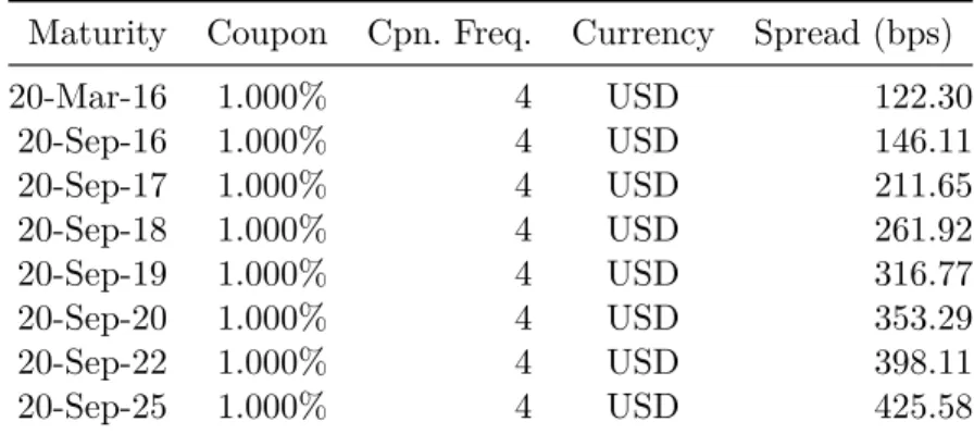
For bonds in USD, the prices were collected from aBloomberg Terminal in July 21, 2015 (Table 5). The same process is applied for CDS curves available, showed in Table6.
Maturity Coupon Cpn. Freq. Price Currency Yield
11-Jan-16 6.250% 2 102.11 USD 1.6620% 23-Jan-17 6.250% 2 105.02 USD 2.8020% 15-Sep-19 5.625% 2 107.75 USD 3.5900% 15-Sep-20 4.625% 2 102.97 USD 3.9798% 11-Jan-22 4.375% 2 96.10 USD 5.0900% 17-Jan-34 8.250% 2 109.50 USD 7.3039% 21-Nov-36 6.875% 2 94.65 USD 7.3746% 10-Nov-39 6.875% 2 93.54 USD 7.4529%
Table 5 – Vale Corporate Bonds Prices in July 21, 2015. Source: Bloomberg Terminal.
Maturity Coupon Cpn. Freq. Currency Spread (bps)
20-Mar-16 1.000% 4 USD 122.30 20-Sep-16 1.000% 4 USD 146.11 20-Sep-17 1.000% 4 USD 211.65 20-Sep-18 1.000% 4 USD 261.92 20-Sep-19 1.000% 4 USD 316.77 20-Sep-20 1.000% 4 USD 353.29 20-Sep-22 1.000% 4 USD 398.11 20-Sep-25 1.000% 4 USD 425.58
Table 6 – Vale CDS Spreads Curve in July 21, 2015. Source: Bloomberg Terminal.
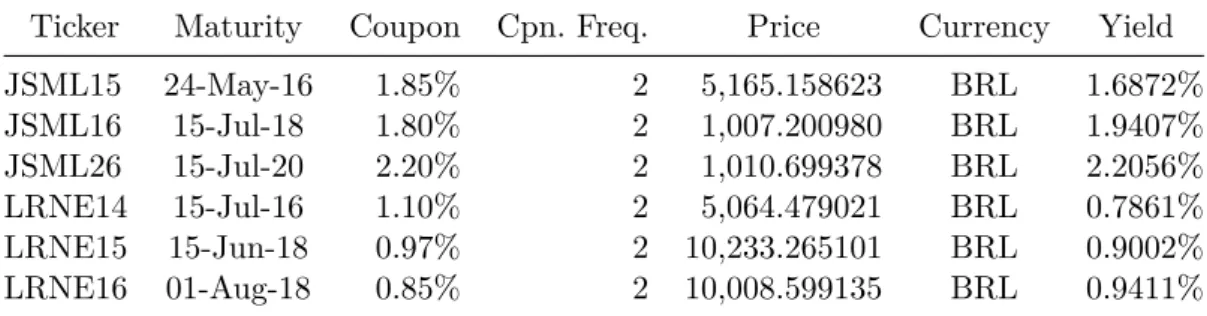
For Debentures, the prices were collected in August 10, 2015, from ANBIMA website9, grouped by their coupon calculation type. Debentures (DI+Spread) are showed
in Table 7. In Table 8, we have the (%DI) debentures and in Table 9 we show the (IPCA+Spread) market prices.
9
Chapter 4. Model Application 34
Ticker Maturity Coupon Cpn. Freq. Price Currency Yield
JSML15 24-May-16 1.85% 2 5,165.158623 BRL 1.6872% JSML16 15-Jul-18 1.80% 2 1,007.200980 BRL 1.9407% JSML26 15-Jul-20 2.20% 2 1,010.699378 BRL 2.2056% LRNE14 15-Jul-16 1.10% 2 5,064.479021 BRL 0.7861% LRNE15 15-Jun-18 0.97% 2 10,233.265101 BRL 0.9002% LRNE16 01-Aug-18 0.85% 2 10,008.599135 BRL 0.9411%
Table 7 – Debentures Prices (DI+Spread) in August 10, 2015. Source: ANBIMA.
Ticker Maturity Coupon Cpn. Freq. Price Currency Yield
JSML18 15-Jun-19 116.00% 2 1,021.758883 BRL 116.6292% JSML38 15-Jun-21 118.50% 2 1,022.727726 BRL 118.9221%
Table 8 – Debentures Prices (%DI) in August 10, 2015. Source: ANBIMA.
Ticker Maturity Coupon Cpn. Freq. Price Currency Yield
JSML36 15-Jul-20 7.50% 1 1,105.730202 BRL 9.1189% JSML28 15-Jun-21 8.00% 1 1,055.097329 BRL 9.3931% LRNE24 15-Jul-17 7.80% 1 8,773.173913 BRL 7.5578% LRNE25 15-Jun-19 5.70% 1 11,824.054184 BRL 8.1253% VALE18 * 15-Jan-21 6.46% 1 1,175.626526 BRL 6.3407% VALE28 * 15-Jan-24 6.57% 1 1,178.433162 BRL 6.4473% VALE38 * 15-Jan-26 6.71% 1 1,190.899791 BRL 6.4583% VALE48 * 15-Jan-29 6.78% 1 1,204.073128 BRL 6.4022%
Table 9 – Debentures Prices (IPCA+Spread) in August 10, 2015. Source: ANBIMA.
Chapter 4. Model Application 35
4.3 Application
In this Section, we show one detailed example of the model application done in this work, in which we analyze Vale corporate bonds and Vale CDS Curve, which we have called Cross-Instruments Analysis.
4.3.1 Vale USD Bonds and Vale CDS Spreads - July 21, 2015
In Figure1, we analyzed the Implied Piece-Wise Constant Risk-Neutral Mean Loss Rate, HtLt, extracted from Vale bonds in USD. This curve represents the conditional
Risk-Neutral Mean Loss Rates implied by market prices, which is the product of the conditional probability of default Ht and its fractional lossLt. Since each maturity has its
bid/offer spread, we can observe some irregularity with the Curve being upward slopping until July 2021, decreasing after the maturity of July 2033, and going back up until the end of curve.
Figure 1 – HtLt Piece-Wise Constant from Vale Corporate Bonds in USD.
Chapter 4. Model Application 36
Since most of CDS dealers are net-sellers and non-dealers are net-buyers10, one possible
explanation to this difference in HtLt is that dealers charge a large premium to sell this
kind of insurance.
Figure 2 – HtLt Piece-Wise Constant from Vale CDS Spreads in USD.
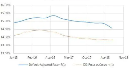
Now we will analyze the Implied Term-Structures of Interest Rates,Rt, (Equation
3.4) from Vale corporate bonds in Figure 3plotted against the time t in days. This curve
is composed by the Default-Free Interest Rate Curve, which is also included in the chart, and the Piece-Wise Constant Function Risk-Neutral Mean Loss Rate, where we can see the consequences of the irregularity cited earlier.
Figure 3 – Implied Term-Structure of Interest Rates from Vale Corporate Bonds in USD.
10
Chapter 4. Model Application 37
The Figure 4shows the same curves implied by Vale CDS Spreads. Their upward slopping shape is reflected in Rt and also their higher levels ofHtLt mentioned recently.
In this case, although Vale Corporate Bonds and its CDS Spread Curve share the same
Default-Free Interest Yield Curve (defined the Section 4.2.1), this is not a pattern on the rest of the analysis in this work.
Figure 4 – Implied Term-Structure of Interest Rates from Vale CDS Spreads in USD.
Finally, in Figure 5we present theCumulative Risk-Neutral Mean Loss Rate, HtLt,
implied by Vale corporate bonds, which represents the cumulative distribution function given by:
F(x) = ✶x≥0
(
1−e−Pxt=1λ )
=✶x≥0
(
1−e−Pxt=1HtLt )
whereHtLt is the Piece-Wise Constant from Equation 3.5 and x is the number of
Chapter 4. Model Application 38
Figure 5 – Cumulative HtLt from Vale Corporate Bonds in USD.
Figure 6 shows the Cumulative Risk-Neutral Mean Loss Rate from Vale CDS Spreads11. Prior we have exposed the Implied Piece-Wise ConstantH
tLt, function extracted
from Vale CDS Spreads are multiple times higher than the ones from Vale Corporate Bonds and these differences are reflected in this chart as well: the Cumulative Risk-Neutral Mean Loss Rate for 3,500 days is 60%, against 25% extracted from Vale Corporate Bonds.
Figure 6 – Cumulative HtLt from Vale CDS Spreads in USD.
11
This CumulativeHtLt rate modeled in this paper is different from theDefault Probabilitycalculated
from a Bloomberg Terminal, that is simply given by P(t) = 1−exp−t
CDS L
Chapter 4. Model Application 39
From our model perspective, if we want to take on Vale’s credit risk in USD, we should consider doing it via CDS. Although there is some counterparty risk in CDS trading, the differences between HtLt extracted from bonds and CDS Spreads are so large that
40
5 Empirical Results
5.1 Presentation
According to the framework defined previously (Section 4.3.1), we present the results grouped by their cases:Cross-Instruments Analysis andTax-Exempt Debentures. In the latter, since the income taxes are exempted, debentures trade below their Default-Free Interest Rate Curve. In this analysis, we use the interval of 22.5% to 15.0%1 to apply a
flat discount in their respective Default-Free Interest Rate Curve.
5.2 Cross-Instruments Analysis
5.2.1 LRNE DI+Spread and IPCA+Spread Debentures in BRL - August 10,
2015
Looking at the Figures7 and 8, we see the Implied Piece-Wise Constant HtLt for
LRNE DI-Linked and IPCA-Linked Debentures, respectively, and we can observe that while the DI-Linked Debentures have a steadyHtLt, around 1% along the whole chart, the
IPCA-Linked Debentures have a much lower Risk-Neutral Mean Loss Rate in short-term, which spikes after July 2017, achieving HtLt= 2.30%.
Figure 7 – HtLt Piece-Wise Constant from LRNE (DI+Spread) Debentures in BRL.
1
Chapter 5. Empirical Results 41
Figure 8 – HtLt Piece-Wise Constant from LRNE (IPCA+Spread) Debentures in BRL.
Next, we show their Implied Term-Structures of Interest Rates in Figures9and 10. In the latter, we can see the consequences of that spike when we look at the difference with their Default-Free Interest Rate Curve. Note that they do not share the same rt.
Chapter 5. Empirical Results 42
Figure 10 – Implied Term-Structure of Interest Rates from LRNE (IPCA+Spread) Deben-tures in BRL.
Figures11and12exhibit the CumulativeHtLt. Since DI-Linked Debentures mature
shortly after 700 days, we are not able to see the consequences of the differences exposed in the previous charts. In that way, the analysis had to be restricted within this time span. So, if we want to take on LRNE credit risk, the best choice is to do it via DI-Linked Debentures, where the Implied HtLt is higher.
Chapter 5. Empirical Results 43
Figure 12 – Cumulative HtLt from LRNE (IPCA+Spread) Debentures in BRL.
5.2.2 JSML DI+Spread, %DI and IPCA+Spread Debentures in BRL - August
10, 2015
In our sample, JSML is the only company that has DI+Spread, %DI and IPCA+Spread Debentures. Analyzing Figures 13 and 14, we can observe that, in short-term, DI+Spread and %DI have similar Implied Piece-Wise Constant, HtLt. However, after June 2019, the
%DI has a much higher Implied Risk-Neutral Mean Loss Rate (HtLt= 4.69%).
Addition-ally, IPCA+Spread Debentures (Figure 15) shows an even higher HtLt of 6.63%, after
July 2020. One possible explanation is that we have used "closing prices". In that way, if the short-term IPCA+Spread is priced with a low Risk-Neutral Mean Loss Rate, it reflects on the term-structure of long-term IPCA+Spread and results in a spike on its HtLt in the
end of the curve.
Figures16and17present their respective Implied Term-Structures of Interest Rates that share a same Default-Free Interest Rate Curve. Although their shapes are similar, we can observe the consequences of the higher HtLt of the %DI Debentures comparing them
Chapter 5. Empirical Results 44
Figure 13 – HtLt Piece-Wise Constant from JSML (DI+Spread) Debentures in BRL.
Figure 14 – HtLt Piece-Wise Constant from JSML (%DI) Debentures in BRL.
Lastly, their Cumulative Risk-Neutral Mean Loss Rates are in Figures19, 20and
21. Comparing the first two, until 1,200 days, we cannot observe significant disparity between them. In the last two, we can extend the analysis until 1,400 days and recognize a small difference, 12% against 10%. Therefore, if we are willing to take on JSML credit risk, there is a higher HtLt in the medium-term (until June 2019) for %DI Debentures
Chapter 5. Empirical Results 45
Figure 15 – HtLt Piece-Wise Constant from JSML (IPCA+Spread) Debentures in BRL.
Chapter 5. Empirical Results 46
Figure 17 – Implied Term-Structure of Interest Rates from JSML (%DI) Debentures in BRL.
Chapter 5. Empirical Results 47
Figure 19 – Cumulative HtLt from JSML (DI+Spread) Debentures in BRL.
Chapter 5. Empirical Results 48
Chapter 5. Empirical Results 49
5.3 Tax-Exempt Debentures Analysis
5.3.1 Vale (IPCA+Spread) Debentures in BRL - August 10, 2015
Looking at the yields of Vale debentures in Table9, we can see that they trade below their Default-Free Interest Rate Curve (Table 4). This is because they are Tax-Exempt. One way the Brazilian Government had been trying to stimulate infrastructure investment is by giving incentives to the debt-holder, like tax-exemptions for individual investors, and we have analyzed how the market implies the Risk-Neutral Mean Loss to this type of debt.
Applying our model directly would result in negative values for the Implied Piece-Wise Constant HtLt, a fact that does not make sense either mathematically, given that
HtLt is, by definition, a probability, or economically, because Vale’s credit risk should not
be lower than its respective sovereign risk, which is assumed as default-free. To circumvent this tax-exemption for individual investors, first we have applied a flat discount of 22.5% in the Default-Free Interest Rate Curve and then we use a 15.0% discount in the same curve, considering that individual investor could keep the investment for at least two years.
Figure 22 – HtLt Piece-Wise Constant from Vale (IPCA+Spread) Debentures in BRL (22.5% Tax-Discount).
The Figure 22 shows the first case, with 22.5% Discount. The 15.0% Tax-Discount is in Figure 23, which shows that, even with the adjustments made on their
Default-Free Interest Rate Curve, their Implied Piece-Wise Constant HtLt is considerably
lower compared with the other debentures analyzed previously and it results in an Implied
Chapter 5. Empirical Results 50
Figure 23 – HtLt Piece-Wise Constant from Vale (IPCA+Spread) Debentures in BRL (15.0% Tax-Discount).
Lastly, Figures24 and25show their Implied Term-Structure and Figures 26and27
present their Cumulative HtLt. With 22.5% Tax-Discount, we can see that for 3,000 days,
the Cumulative HtLt is at 10.0%. With the 15.0% Tax-Discount, for the same period, the
Cumulative HtLt is at 4.5%. Comparing these with the one implied by Vale Bonds in USD
of 20.0% (Figure 5), we can conclude that, at these levels, we should be exposed to Vale’s credit risk using other securities, bond and CDS, and not these Tax-Exempt Debentures, according to our model.
Chapter 5. Empirical Results 51
Figure 25 – Implied Term-Structure of Interest Rates from VALE (IPCA+Spread) Deben-tures in BRL (15.0% Tax-Discount).
Chapter 5. Empirical Results 52
Part III
54
6 Conclusion
We presented a model useful to extract hazard rates from a Risk-Neutral Mean Loss Rate curves implied by market prices. The model is based on Duffie and Singleton
(1999), using a Piece-Wise Constant Function with N parts, when information is available,
to imply the term-structure of interest rates, as proposed by Meres and Almeida (2008). The objective of this work is to implement this framework to analyze Brazilian Corporate Debt, composed by Bonds in USD, CDS Spreads and Debentures.
First, we have defined theDefault-Free Yield Curve compatible with each security and selected the data grouped by issuer, currency, coupon calculation type and payment seniority. Then, we have estimated the Risk-Neutral Mean Loss Rate curve that would fit the market prices and, therefore, it is an arbitrage-free model. Based on the extracted Risk-Neutral Mean Loss Rates Curves, we took a deeper look in two different situations:
Cross-Instruments Analysis, represented by Vale Bonds and CDS Curves in USD, LRNE Debentures with different coupon calculation type, DI+Spread and IPCA+Spread and JSML Debentures (DI+Spread, %DI and IPCA+Spread). In the first case, we showed that is better to be exposed in credit risk via CDS. In the second, we chose the DI-Linked Debentures. For JSML, the choices are relative to the time-period: until medium-term, we chose the %DI Debentures and in the long-term we favor the IPCA+Spread Debentures;
Tax-Exempt Debentures Analysis, we exposed the case of infrastructure debt that have a tax exemption for individual investors, represented by Vale Debentures in BRL. Even though we have considered 15.0% to 22.5% discounts in their Default-Free Yield Curve, we should not take on the company’s credit risk for such premium, based in our model.
The limitations of the framework applied are that the analyses were made with "closing prices", so there is no bid/offer considered, so the HtLt could change. There is a
tight restriction on the Duffie and Singleton (1999) that assumes the security price does not jump when the default really occurs and we did not test to see how the model would behave when this condition fails to hold.
55
7 Future Work
Using this model, it is possible to make a sensitivity analysis on the fractional loss
Lt, varying within an interval and see the consequences on their respective Risk-Neutral
Mean Loss Rate Curve. Although the Brazilian bankruptcy law changed recently, another suggestion is to make an empirical estimation of the fractional loss Lt according to the
issuer’s industry, like Altman and Kishore (1996) did for the U.S. bond market. These estimations would help identifying Ht and Lt separately. Additionally, it is possible to
stress the model with "shocks" in the Default-Free Yield Curve, like a sudden change in monetary policy, or "shocks" in the yield-to-maturity, like aflight to safety situation, to see how the Risk-Neutral Mean Loss Rates implied by the market changed in these scenarios. In a similar way, it is promising to look at the times when these scenarios happened historically and see if the decisions on which instrument to take on the credit risk would hold after the scenario took place.
One way to expand this work is to use the model proposed by Collin-Dufresne, Goldstein and Hugonnier (2004), which is not restricted by the no-jump condition in the arrival of default. Since they argued that their model performs better in scenarios of flight to quality, counterparty risk and the systematic jump risk, an idea is to compare their model with the one proposed in this work, based on Duffie and Singleton (1999), and see how critical this restriction is for this model.
From a trading perspective, it is possible to use the same model proposed in this work to make a strategy, assuming a fractional loss Lt, run a backtest with the portfolio
and see if it performs better than a buy-and-hold position on the same securities.
Moreover, a promising way to study this is using of a proprietary credit system to estimate the credit risk and the company’s hazard rate, compare with the implied hazard rate to see if the decisions are different from the framework proposed in this work and analyze the performance of this portfolio overtime.
56
Bibliography
ALTMAN, E. I.; KISHORE, V. M. Almost everything you wanted to know about recoveries on defaulted bonds. Financial Analysts Journal, CFA Institute, v. 52, n. 6, p. 57–64, 1996.
CARATORI, B. M. Risco soberano e probabilidade de default implícita em swaps de crédito. 2008.
COLLIN-DUFRESNE, P.; GOLDSTEIN, R.; HUGONNIER, J. A general formula for valuing defaultable securities. Econometrica, Wiley Online Library, v. 72, n. 5, p. 1377–1407, 2004.
COX, J. C.; INGERSOLL, J. E.; ROSS, S. A. A theory of the term structure of interest rates. Econometrica, World Scientific, v. 53, n. 2, p. 385–407, 1985.
DIEBOLD, F. X.; LI, C. Forecasting the term structure of government bond yields. Journal of econometrics, Elsevier, v. 130, n. 2, p. 337–364, 2006.
DUFFIE, D.; LANDO, D. Term structures of credit spreads with incomplete accounting information. Econometrica, JSTOR, p. 633–664, 2001.
DUFFIE, D.; SINGLETON, K. J. Modeling term structures of defaultable bonds. Review of Financial studies, Soc Financial Studies, v. 12, n. 4, p. 687–720, 1999.
FABOZZI, F. J.; MANN, S. V. The handbook of fixed income securities. [S.l.]: McGraw Hill Professional, 2012.
FERNANDEZ, P. R. S. Probabilidade implícita de default em debêntures do mercado brasileiro. 2014.
GIESECKE, K. Credit risk modeling and valuation: An introduction. Available at SSRN 479323, 2004.
LITTERMAN, R. B.; IBEN, T. Corporate bond valuation and the term structure of credit spreads. The journal of portfolio management, Institutional Investor Journals, v. 17, n. 3, p. 52–64, 1991.
MERES, B.; ALMEIDA, C. Extracting default probabilities from sovereign bonds. Brazilian Review of Econometrics, v. 28, n. 1, p. 77–94, 2008.
MERTON, R. C. On the pricing of corporate debt: The risk structure of interest rates. The Journal of Finance, Wiley Online Library, v. 29, n. 2, p. 449–470, 1974.
NELSON, C. R.; SIEGEL, A. F. Parsimonious modeling of yield curves. Journal of business, JSTOR, p. 473–489, 1987.
Bibliography 57
SHAREF, E.; FILIPOVIĆ, D. Conditions for consistent exponential-polynomial forward rate processes with multiple nontrivial factors. International Journal of Theoretical and Applied Finance, World Scientific, v. 7, n. 06, p. 685–700, 2004.