Rafael de Braga Castilho
Estimation of random coefficients logit
demand models: an application to the
Brazilian fixed income fund market
Estimation of random coefficients logit
demand models: an application to the
Brazilian fixed income fund market
Dissertação para obtenção do grau de mestre apresentada à Escola de Pós-Graduação em Economia
Área de concentração: Organização Indus-trial
Orientador: Luis Henrique Bertolino Braido
Cistilho, Rifiel de Brigi
Estimition of rindom coefficients logit demind models : ni ipplicition to the Briziliin fixed income frnd mirket / Rifiel de Brigi Cistilho. – 2013.
30 f.
Dissertição (mestrido) - Frndição Getrlio Virgis, Escoli de Pós-Gridrição em Economii.
Orientidor: Lris Henriqre Bertolino Briido. Inclri bibliogrifii.
1. Orginizição indrstriil. 2. Oferti e procrri. 3. Demindi (Teorii econômici). 4. Frndo mútro de rendi fixi. I. Briido, Lris H. B. II. Frndição Getrlio Virgis. Escoli de Pós- Gridrição em Economii. III. Títrlo.
Estimação de demanda e oferta em mercados com produtos diferenciados é uma questão central em organização industrial empírica e tem sido usada para estudar os efeitos de taxas, fusões, introdução de novos bens, poder de mercado, dentre outros. Logit e Logit com coeficientes aleatórios são exemplos de modelos de demanda utilizados para estudar estes efeitos. Para a oferta geralmente é suposto equilíbrio de Nash em preços. Este trabalho apresenta uma discussão detalhada destes modelos de demanda e oferta, assim como o procedimento para estimação. Por fim é feita uma aplicação para o mercado brasileiro de fundos de renda fixa.
Estimation of demand and supply in differentiated products markets is a central issue in Empirical Industrial Organization and has been used to study the effects of taxes, merges, introduction of new goods, market power, among others. Logit and Random Coefficients Logit are examples of demand models used to study these effects. For the supply side it is generally supposed a Nash equilibrium in prices. This work presents a detailed discussion of these models of demand and supply as well as the procedure for estimation. Lastly, is made an application to the Brazilian fixed income fund market.
List of Figures
1 Total Net Asset . . . 17
2 Number of Funds . . . 17
List of Tables
1 Descriptive Statistics . . . 162 Results from Logit Demand . . . 18
3 Results from Marginal Cost Pricing . . . 19
4 Results from Demand and Supply Side in RC-Logit . . . 20
Contents
1 Introduction 2 2 Literature Review 2 3 Demand Side 3 3.1 Utility and Demand . . . 33.2 Logit . . . 5
3.3 Random Coefficients Logit . . . 7
4 Supply Side 7 5 Estimation and Endogeneity 8 5.1 Logit . . . 10
5.2 Random Coefficients Logit . . . 11
6 Computation 12 7 Application 15 7.1 Fixed Income Market . . . 15
7.2 Data . . . 16
7.3 Results. . . 17
8 Conclusion 20
Bibliography 22
1 Introduction
Estimation of demand in differentiated products markets is a central issue in Empirical In-dustrial Organization. This dissertation presents a detailed discussion of two prominent demand models of differentiated products: Logit and Random Coefficients (RC) Logit. These two models were first presented at McFadden (1974) and Berry et al. (1995) respectively. Its applications includes studying the effects of taxes, merges, introduction of new goods, market power, among others.1
RC-Logit model is computationally more demanding than Logit. The integral defining the market share does not have a closed form and simulation is necessary. Moreover in order to consider the endogeneity of prices and unobserved product characteristics and then apply the method of moments for estimation it is necessary to invert numerically the market share function. This procedure was first presented inBerry(1994), which deals with the existence and uniqueness of the vector of unobserved characteristics, while the iteration to obtain this vector is suggested at Berry et al.(1995). Both procedures are described in detail.
Note that these models require only aggregate data on prices, quantity and product charac-teristics, although demographic data are advisable. When available, individual data also have been used, see for exampleBerry et al.(2004a).
After presenting these models, is made an application to the Brazilian fixed income market utilizing data provided by the Brazilian Financial and Capital Markets Association (Anbima). Four cases were employed: Logit demand with and without considering endogeneity; marginal cost pricing and RC-Logit with supply.
Section2 presents the characteristic and the product based demand models, highlighting its advantages, disadvantages and limitations. Section3introduces the consumer decision problem, Logit and RC-Logit demand models, while Section4models the supply side. Section5discuss the procedure for estimation of these two demand models and how endogeneity is treated. Section6
shows the details of the MATLAB code2 for estimation of RC-Logit, followed by an application
to the Brazilian fixed income market in Section 7. Section8 concludes and proposes extensions.
2 Literature Review
In a differentiated products market with 𝑁 products and a representative agent with
prefer-ences over products, the system of demand would be like
𝑞1 = 𝛼1+
𝑁
∑︁
𝑘
𝜂1𝑘𝑝𝑘+𝜖1
...
𝑞𝑁 = 𝛼𝑁 +
𝑁
∑︁
𝑘
𝜂𝑁 𝑘𝑝𝑘+𝜖𝑁
This approach has some problems. The number of parameters to be estimated grows quadrat-ically in the number of products, i.e. if there are𝑁 goods, it requires the estimation of𝑁*(𝑁+1)
parameters. This could be too large, for example a market with 10 goods has 110 parameters to be estimated. Another problem is the impossibility to analyse the demand for new goods prior to their introduction, which could bring information on the incentives for new entries.
The too many parameters estimation problem and the impossibility of evaluating the in-troduction of new goods comes from the fact that preferences are over the products, non its characteristics.
The characteristics based or hedonic model of demand is one such that the preferences are over the characteristics of the products, i.e. each product is defined as a bundle of characteristics and the preferences are over these characteristics. As usual, the product chosen is the one which maximizes consumer utility. This system of demand would be like
𝑞1 =
𝐾
∑︁
𝑘
𝜂𝑘𝑥1𝑘+𝜖1
...
𝑞𝑁 = 𝐾
∑︁
𝑘
𝜂𝑘𝑥𝑁 𝑘+𝜖𝑁
where 𝑥𝑛 ∈ R𝐾 is the vector of observed characteristics of product 𝑛 and therefore it is only
necessary to estimate 𝐾 parameters, regardless on the number of products 𝑁. Moreover the
demand for a new product which has the same observed characteristics can be predicted since the coefficients𝜂 does not change among products.
Examples of these are Logit and RC-Logit demand models, presented inMcFadden(1974) and
Berry et al.(1995) respectively. The first keeps the representative agent approach so preferences for each of the observable characteristic are the same across agents, while the second relaxes this hypothesis (as will be explained in detail) but with a computational cost.
Papers utilizing RC-Logit demand to understand features of a specific market have been published in main journals. Levinsohn et al. (1999) evaluates the voluntary export restraint that was placed by the United States on exports of automobiles from Japan. Nevo(2001) and
Nevo(2000a) analyse the read-to-eat cereal industry, the first investigates if conduct is collusive or competitive, while the second simulates mergers between firms and the predicted effect on profits and consumer welfare. Petrin(2002) studies the effects of the introduction of minivan on consumer welfare and profits of producer and non-producer firms.
As commented inAckerberg et al. (2007), it is important to note that hedonic models have limitations. Even considering unmeasured characteristics, if the researcher does not have ac-cess, or chooses wrongly the characteristics, this model does not provide a good prediction of substitution between goods.
In relation to the new goods problem, the hedonic model can only provide information on products which has the same observables characteristics. However many new products consists of a bundle of characteristics different from the previously available or could be predicted by the researcher. One example is the smartphone, which combines cellphone, camera and access to internet. Demand for this product cannot be predicted until the first smartphone was present in the market, since this product does not fit in a model of demand for each one of these products isolated.
3 Demand Side
In this section we characterize the hedonic demand model. First describing utility and con-sumer decision problem. Then the particular cases of Logit and RC-Logit are presented.3
3.1 Utility and Demand
There is a market with 𝑖 = 1, . . . , 𝐼 consumers and 𝑗 = 0, . . . , 𝐽 goods. We only observe
aggregate data on quantities, average prices and product characteristics, i.e. there is no data on individual purchases.
The utility consumer 𝑖receives from consuming good 𝑗 is given by
𝑈(𝜁𝑖, 𝑥𝑗, 𝜉𝑗;𝜃)
where𝜁𝑖is a vector of individual characteristics,𝑥𝑗 = (˜𝑥𝑗,𝑝𝑗)and𝜉𝑗 are respectively the observed
and unobserved (by the econometrician) product characteristics, 𝑝𝑗 is the price, 𝜉𝑗 represents
quantifiable characteristics that are not available in the data and unquantifiable characteristics like prestige and reputation. Finally, 𝜃is a vector of parameters to be estimated.
Utility obtained from consuming a good depends on the product characteristics and the consumer taste for each of these characteristics. Then agents with different tastes may choose different products.
As a discrete choice model, each consumer must choose one unit of one good available in the market. To allow the possibility of not buying any of the𝐽 goods,𝑗= 0is defined as the outside
good, which can be thought as the consumer ability to substitute to other markets. Note that without this outside good, a homogeneous increase in the price of all goods does not change the market demand.
Consumer𝑖chooses good 𝑗 if and only if:
𝑈(𝜁𝑖,˜𝑥𝑗, 𝑝𝑗, 𝜉𝑗;𝜃)>𝑈(𝜁𝑖,˜𝑥𝑟, 𝑝𝑟, 𝜉𝑟;𝜃) for each 𝑟= 0,1, ..., 𝐽
The set of 𝜁 that induces the choice of good𝑗 is then:
𝐴𝑗 ={𝜁 :𝑈(𝜁,˜𝑥𝑗, 𝑝𝑗, 𝜉𝑗;𝜃)>𝑈(𝜁,𝑥˜𝑟, 𝑝𝑟, 𝜉𝑟;𝜃), for 𝑟 = 0,1, ..., 𝐽}
and given the populational density of𝜁,P0(d𝜁). The market share of good𝑗 is given by
𝑠𝑗(˜𝑥,𝑝, 𝜉;𝜃,P0) = ∫︁
𝜁∈𝐴𝑗
P0(d𝜁)
A particular case of the utility defined above is:
𝑈(𝜁𝑖,˜𝑥𝑗, 𝑝𝑗, 𝜉𝑗;𝜃)≡𝛿𝑗𝑡(˜𝑥𝑗,𝑝𝑗,𝜉𝑗;𝜃1) +𝜇𝑖𝑗(𝜁𝑖,˜𝑥𝑗,𝑝𝑗;𝜃2) +𝜖𝑖𝑗
with:
𝛿𝑗(˜𝑥𝑗,𝑝𝑗,𝜉𝑗;𝜃1) = ˜𝑥𝑗𝛽−𝛼𝑝𝑗+𝜉𝑗
𝜇𝑖𝑗(𝜁𝑖,˜𝑥𝑗,𝑝𝑗;𝜃2) = ∑︁
𝑘
𝑥𝑗𝑘(𝛽𝑘𝑠𝜈𝑖𝑘+𝛽𝑘𝑑1𝑑𝑖1+𝛽𝑘𝑑2𝑑𝑖2+. . .+𝛽𝑘𝐷𝑑 𝑑𝑖𝐷)
𝜁𝑖= (𝜈𝑖,𝑑𝑖,𝜖𝑖) = (𝜈𝑖1,𝜈𝑖2, . . . ,𝜈𝑖𝐾,𝑑𝑖1,𝑑𝑖2, . . . ,𝑑𝑖𝐷,𝜖𝑖0,𝜖𝑖1,𝜖𝑖2, . . . , 𝜖𝑖𝐽)
𝛿𝑗 is the mean utility of good 𝑗, while 𝜇𝑖𝑗 is the individual 𝑖 deviation from that mean. The
term 𝜇𝑖𝑗 captures the interactions between consumer and product characteristics. Individual
characteristics𝜁𝑖are comprised of individual shocks𝜈𝑖𝑘for each of the𝐾observed characteristics,
vector of demographics𝑑𝑖 and a vector𝜖𝑖 of additive shocks to utility. More details on the term
𝜇𝑖𝑗 are presented in the RC-Logit subsection.
The vector 𝜃 of parameters is divided into two parts: 𝜃1 = (𝛼,𝛽) associated with the mean
value 𝛿 and 𝜃2 = (𝛽𝑠, 𝛽𝑑) with the deviation from that mean. The reason for this division will
3.2 Logit
In the Logit specification 𝜇𝑖𝑗 = 0 ∀ 𝑖,𝑗 so all consumers have the same preferences and
utility is given by
𝑈(𝜁𝑖,𝑥˜𝑗,𝑝𝑗, 𝜉𝑗;𝜃) = ˜𝑥𝑗𝛽−𝛼𝑝𝑗 +𝜉𝑗+𝜖𝑖𝑗 =𝛿𝑗 +𝜖𝑖𝑗
where𝜖𝑖𝑗 𝑖𝑖𝑑
∼ type I extreme value.4 Consumer𝑖 chooses𝑗 iff
𝑈(𝜁𝑖,˜𝑥𝑗,𝑝𝑗, 𝜉𝑗;𝜃)>𝑈(𝜁𝑖,˜𝑥𝑟, 𝑝𝑟, 𝜉𝑟;𝜃) , ∀ 𝑟̸=𝑗
with this utility specification, it is equivalent to
𝛿𝑗−𝛿𝑟+𝜖𝑗 >𝜖𝑟 , ∀𝑟 ̸=𝑗
Given a realization of 𝜖𝑗, the probability of choosing 𝑗 given𝜖𝑗 is given by
P𝑗|𝜖𝑗 =
∏︁
∀𝑟̸=𝑗
𝐹(𝛿𝑗−𝛿𝑟+𝜖𝑗)
integrating over𝜖𝑗 we have that
𝑠𝑗 =
∫︁
P𝑗|𝜖𝑗𝑓(𝜖𝑗) d𝜖𝑗
This integral has closed form and (as shown inMcFadden(1974)5) equals6
𝑠𝑗 =
𝑒𝛿𝑗
∑︀𝐽
𝑟=0𝑒𝛿𝑟
To see this note that:
𝑠𝑗 =
∫︁
P𝑗|𝜖𝑗𝑓(𝜖𝑗)𝑑𝜖𝑗
= ∫︁ (︂
∏︁
𝑟̸=𝑗
𝐹(𝛿𝑗−𝛿𝑟+𝜖𝑗)
)︂
𝑓(𝜖𝑗)𝑑𝜖𝑗
= ∫︁ (︂
∏︁
𝑟̸=𝑗
𝑒−𝑒−(𝛿𝑗−𝛿𝑟+𝜖𝑗) )︂
𝑒−𝜖𝑗𝑒−𝑒−𝜖𝑗 𝑑𝜖
𝑗 = ∫︁ exp (︂ −∑︁ 𝑟
𝑒−(𝛿𝑗−𝛿𝑟+𝑣)
)︂
𝑒−𝑣𝑑𝑣, where𝑣=𝜖𝑗 and note that𝛿𝑗−𝛿𝑗 = 0
= ∫︁
exp (︂
−𝑒−𝑣∑︁
𝑟
𝑒−(𝛿𝑗−𝛿𝑟)
)︂ 𝑒−𝑣𝑑𝑣
let𝑡≡exp(−𝑣), then:
𝑑𝑡=−exp(−𝑣)𝑑𝑣 ,𝑣→+∞ =⇒ 𝑡→0,𝑣→ −∞ =⇒ 𝑡→+∞
4This distribution has CDF:𝐹(𝑡) =𝑒−𝑒−t
5McFadden’s version does not include the unobserved vector of characteristics𝜉, but this fact does not change
the logic of the demonstration.
6If 𝜖 ∼𝑁(0,Σ) we fall into the multinomial probit model where this integral has no closed form and then
𝑠𝑗 =
∫︁ 0
+∞
exp (︂
−𝑡∑︁
𝑟
𝑒−(𝛿𝑗−𝛿𝑟)
)︂ (−𝑑𝑡)
=
∫︁ +∞
0
exp (︂
−𝑡∑︁
𝑟
𝑒−(𝛿𝑗−𝛿𝑟)
)︂ 𝑑𝑡
= exp
(︀ −𝑡∑︀
𝑟𝑒−(𝛿𝑗−𝛿𝑟)
)︀
−∑︀
𝑟𝑒−(𝛿𝑗−𝛿𝑟)
⃒ ⃒ ⃒ ⃒ ⃒ +∞ 0
= ∑︀ 1
𝑟𝑒−(𝛿𝑗−𝛿𝑟)
= 𝑒
𝛿𝑗
∑︀
𝑟𝑒𝛿𝑟
Normalizing the outside good to have mean utility zero, i.e. 𝛿0 = 0,7 the market share
becomes
𝑠𝑗(𝑝, 𝑥, 𝜉, 𝜃, 𝑃0) = 𝑒
𝛿𝑗
(1 +∑︀𝐽
𝑗=1𝑒𝛿𝑗)
A property present in Logit model is the Independence of Irrelevant Alternatives (IIA), which in some situations generates substitution patterns different from that expected. The IIA implies that the ratio of the probability of two alternatives being chosen is independent of the others alternatives. This is straightforward, since
𝑠𝑗
𝑠𝑘
=
𝑒𝛿𝑗
(1 +∑︀𝐽
𝑗=1𝑒𝛿𝑗) 𝑒𝛿𝑘
(1 +∑︀𝐽
𝑗=1𝑒𝛿𝑗) = 𝑒
𝛿𝑗
𝑒𝛿𝑘
Note that elasticity of demand for product 𝑗 with respect to the price of product𝑘, denoted
by 𝜀𝑗𝑘, is given by
𝜀𝑗𝑘 =
𝜕𝑠𝑗 𝜕𝑝𝑘 𝑝𝑘 𝑠𝑗 = {︃
−𝛼𝑝𝑗(1−𝑠𝑗) if 𝑗 =𝑘
𝛼𝑝𝑘𝑠𝑘 if 𝑗̸=𝑘
Then cross-price elasticity does not depend on the characteristics of product 𝑗 and own-price
elasticity is crescent (in absolute value) in price, so markup decreases with higher prices. Two examples illustrate how is the substitution generated by Logit model.
Firstly, the known red bus/blue bus problem. Suppose a citizen can go work using a car or a blue bus and that P𝑐 = P𝑏𝑏 = 1/2 - so P𝑐/P𝑏𝑏 = 1 - where P𝑐 and P𝑏𝑏 are the probability of
using the car and the blue bus, respectively.
Now consider that a red bus is introduced and the citizen thinks it is equivalent to the blue bus, then P𝑏𝑏/P𝑟𝑏 = 1. But IIA implies that P𝑐/P𝑏𝑏 keeps equal to 1 and since we need that
P𝑐+ P𝑏𝑏+ P𝑟𝑏= 1, the probabilities the model predicts areP𝑐 = P𝑏𝑏= P𝑟𝑏= 1/3.
However, it is expected that the probability of taking a car keeps the same and the probability of taking the bus be divided equally between the two kind of buses so: P𝑐 = 1/2andP𝑏𝑏= P𝑟𝑏=
1/2. So Logit model can be extreme unrealistic in predicting the introduction of new products.
The second example is presented in Berry et al. (1995) to illustrate a situation where the cross elasticity of demand, generated by the IIA seems implausible.
7Note that given𝛿, we have that𝛿+𝑘·1
𝐽+1with𝑘∈Rpredicts the same market share. So this normalization
Consider that Yugo (a car of low quality) and Mercedes has the same market share. An increase in the price of BMW has the same effect on the market share of these two cars. What seems unreasonable since Yugo and BMW are not close substitutes as Mercedes and BMW.
This occurs because of the functional form of Logit. Since there are not interaction between individual and product characteristics, all consumers have the same preference for the observ-ables characteristics. This means that the substitution depend on the mean value𝛿 not on the
similarity.
To add this interaction some problems arise and it is the focus of Berry (1994) and Berry et al.(1995). It begins to be presented in the next subsection.8
3.3 Random Coefficients Logit
To allow the interaction between individual and product characteristics consider again the utility function:
𝑈(𝜁𝑖,𝑥˜𝑗, 𝑝𝑗, 𝜉𝑗;𝜃) =𝛿𝑗(˜𝑥𝑗,𝑝𝑗,𝜉𝑗;𝜃1) +𝜇𝑖𝑗(𝜁𝑖,˜𝑥𝑗,𝑝𝑗;𝜃2) +𝜖𝑖𝑗
with
𝛿𝑗(˜𝑥𝑗,𝑝𝑗,𝜉𝑗;𝜃1) = ˜𝑥𝑗𝛽−𝛼𝑝𝑗+𝜉𝑗
and
𝜇𝑖𝑗(𝜁𝑖,˜𝑥𝑗,𝑝𝑗;𝜃2) = ∑︁
𝑘
𝑥𝑗𝑘(𝛽𝑘𝑠𝜐𝑖𝑘+𝛽𝑘𝑑1𝑑𝑖1+𝛽𝑘𝑑2𝑑𝑖2+. . .+𝛽𝑑𝑘𝐷𝑑𝑖𝐷)
the term 𝛿𝑗 was present in the Logit specification and represents the mean utility of good 𝑗.
The term 𝜇𝑖𝑗 captures the individual deviation from this mean utility, therefore preferences
over observable characteristics changes among individuals. This individual characteristics are summarized by the vector𝜁𝑖 with
𝜁𝑖 = (𝜈𝑖,𝑑𝑖,𝜖𝑖) = (𝜈𝑖1,𝜈𝑖2, . . . ,𝜈𝑖𝐾,𝑑𝑖1,𝑑𝑖2, . . . ,𝑑𝑖𝐷,𝜖𝑖0,𝜖𝑖1, . . . , 𝜖𝑖𝐽)
where𝜈𝑖 is a vector of random variables with a parametric distribution, usually𝜈𝑖∽𝒩(0𝐾, 𝐼𝐾).
While 𝑑𝑖 is a vector of consumer demographics characteristics and has a nonparametric
distri-bution known from some data source. Generally𝑑𝑖 includes demographics characteristics such
age, income, sex, education and family size.
Note that interaction between individual and product characteristics has two sources, the shocks 𝜈𝑖 and the demographics 𝑑𝑖, captured by the coefficients 𝛽𝑠 and 𝛽𝑑 respectively. It
is these interactions that deal with the IIA and so generates reasonable own and cross price elasticities.
Next section the supply side is presented, starting with the firm decision problem and finishes with the moment conditions used to estimate the supply side parameters. Although not necessary, supply can be incorporated into the estimation adding the necessary moment conditions. This jointly estimation increases the efficiency of the estimates at the cost of requiring more structure.
4 Supply Side
We suppose there are F multi product firms each one producing some subset 𝒥𝑓 of the 𝐽
products offered, where𝒥𝑓∩ 𝒥𝑓′ =∅ if 𝑓 ̸=𝑓′.
8Two another models that deal with the IIA problem are the Nested Logit and the Multinomial Probit. A
Each firm set its prices to maximize profits given the prices of the others. So profit for firm
𝑓 is given by
Π𝑓 =
∑︁
𝑗∈𝒥𝑓
(𝑝𝑗 −𝐶𝑗)𝑀 𝑠𝑗(˜𝑥,𝑝,𝜉;𝜃)
where𝐶𝑗 is the total cost of producing good 𝑗and𝑀 is the number of consumers in the market.
The FOC for product𝑗 produced by firm𝑓 is given by
𝑠𝑗(˜𝑥,𝑝,𝜉;𝜃) +
∑︁
𝑟∈𝒥𝑓
(𝑝𝑟−𝑚𝑐𝑟)
𝜕𝑠𝑟(˜𝑥,𝑝,𝜉;𝜃)
𝜕𝑝𝑗
= 0
In vector notation the FOCs are written as
𝑠(˜𝑥,𝑝,𝜉;𝜃)−∆(˜𝑥,𝑝,𝜉;𝜃)[𝑝−𝑚𝑐] = 0
with∆𝑗𝑟(˜𝑥,𝑝,𝜉;𝜃) =−
𝜕𝑠𝑟
𝜕𝑝𝑗
1
𝑗𝑟, where1
𝑗𝑟 is a indicator function and assumes value1 if𝑗 and 𝑟
are sold by the same firm and0 otherwise.
The marginal cost is given by9
𝑚𝑐𝑗(𝑥𝑐𝑗,𝜔𝑗;𝛾) =𝑥𝑐𝑗𝛾+𝜔𝑗
𝑥𝑐
𝑗 and 𝜔𝑗 are (respectively) the observed and unobserved cost characteristics and 𝛾 is a vector
of parameters to be estimated. The 𝑥𝑐
𝑗 could include input prices, product characteristics and
the quantity produced which would characterize non-constant returns of scale.
This framework can be questionable in many situations. Note that it is supposed static profit maximization, no uncertainty and that consumers are price takers.
As some elements of 𝑥 are supposed to be correlated with 𝜉, we expect that some elements
of 𝑥𝑐 are correlated with𝜔 and that𝜉 and𝜔 are positively correlated since goods with a higher
unobserved quality might cost more to produce.
To incorporate de supply side in the algorithm just write the FOCs as
∆(˜𝑥,𝑝,𝜉;𝜃)−1𝑠(˜𝑥,𝑝,𝜉;𝜃) =𝑝−𝑚𝑐(𝑥𝑐,𝜔;𝛾)
substitute the𝑚𝑐(𝑥𝑐,𝜔;𝛾)and rearrange to obtain
𝜔 =𝑝−𝑥𝑐𝛾−∆(˜𝑥,𝑝,𝜉;𝜃)−1𝑠(˜𝑥,𝑝,𝜉;𝜃)
For estimation get a set of instruments and then construct a GMM estimator choosing the𝛾
that makes the sample analogue of these moments closest to satisfy the orthogonality conditions. More details are provided in the next section.
5 Estimation and Endogeneity
The endogeneity appears in this setting as it is expected that some observable characteristics present in𝑥are correlated with the unobservable𝜉 as well as some elements of𝑥𝑐 are correlated
with𝜔.
Generally for the demand side it is supposed that location of product characteristics (other than price)𝑥˜are exogenous or at least determined prior to the revelation of consumers valuation
of unobserved product characteristics 𝜉.10 For the supply side, all cost characteristics 𝑥𝑐 are
supposed exogenous to𝜔.
So we are worried about the correlation between price 𝑝 and unobservables 𝜉 and 𝜔. The
direction of bias in the price coefficient can sometimes be determined logically. As exemplified inTrain (2003), price coefficient is biased downward (in modulus) if higher prices are associated with desirable attributes, because the estimated price coefficient captures both price effect and desirable unobserved attributes effects. While opposite direction occurs if a price decrease is made jointly with an increase of advertising. The increased demand comes from both effects and price coefficient is biased upward (in modulus).
But unlike the homogeneous goods case, in differentiated product markets both prices and unobservables enter the demand equation in a nonlinear fashion.11
A procedure one could use is search for the𝛼 and 𝛽 that solve
min𝛼,𝛽 𝑗=𝐽
∑︁
𝑗=1 (︀
𝑆𝑗𝑛−𝑠𝑗(𝛼, 𝛽, 𝜉1, . . . ,𝜉𝐽))︀2
but in addiction to the fact that the𝜉’s are not observed, this procedure ignores endogeneity of
price and then leads to biased estimates.
To avoid the use of nonlinear instrumental variables,Berry et al. (1995) propose a two-step method that consists of an inversion of the market share function to recover the mean utility levels and then an usual instrumental variables regression.
The market share predicted by the model is such that 𝑆𝑛 = 𝑠(˜𝑥,𝑝,𝛿;𝜃) where 𝑆𝑛 is the
observed market share,Berry(1994) proves that under a set of mild conditions there is a one to one relation between the mean values 𝛿 and 𝑆𝑛 = 𝑠(˜𝑥,𝑝,𝛿;𝜃).12 So we can invert this function
and obtain
𝛿(𝑠) = ˜𝑥𝛽−𝛼𝑝+𝜉
and use standard instrumental variables techniques to estimate the unknown parameters, i.e. we run instrumental variables regression of𝛿 on(˜𝑥,𝑝)to estimate(𝛼, 𝛽)treating𝜉 as an error term.
The market share function inversion to obtain 𝛿 in Logit model is easily obtained applying
logarithms and normalizing mean utility of the outside good to zero, while in RC-Logit it needs
10See Berry (1994), Berry et al. (1995), Cohen (2008). While Berry et al. (2004b) presents a more general
version where a product𝑗has𝑥1𝑗∈R𝑑1exogenous characteristics and𝑥2𝑗∈R𝑑2endogenous characteristics. But
the procedure is analogous.
11Suppose we have
Demand: 𝑞𝑑
𝑖 =𝛼1+𝑥′𝑖1𝛽1+𝑢𝑖1
Supply: 𝑝𝑖=𝛼2𝑞𝑠𝑖+𝑥′𝑖2𝛽2+𝑢𝑖2
Equilibrium: 𝑞𝑑 𝑖 =𝑞𝑖𝑠
then𝑢𝑖1is correlated with𝑢𝑖2and𝑝𝑖is endogenous in demand function. Assuming there is a set of instrumental
variables Z - generally the cost shifters𝑥𝑖2 - one can form the moment conditions
E(𝑧𝑖𝑢𝑖1) = 0
and use GMM to estimate the parameters.
12Consider the set of conditions:
1- The predicted market-share function 𝑠(·) is everywhere differenciable with respect to 𝛿 , 𝜕𝑠j
𝜕𝛿j > 0 and
𝜕𝑠j
𝜕𝛿k >0 ∀𝑘̸=𝑗.
2- For all possible values of𝑥, the density of consumer characteristics is strictly positive and continuous for all vector of individual characteristics𝜁.
to be made numerically. This procedure was first presented inBerry et al.(1995).
Solved the non linearity problem, we turn to the choose of appropriate instruments, which are variables correlated with the endogenous variable𝑝 but not with the unobservables𝜉 and𝜔.
Following Berry et al. (1995) we suppose that supply and demand unobservables are mean independent of both observed product characteristics and cost shifters, i.e.
E(𝜉𝑗|𝑥, 𝑥˜ 𝑐) =E(𝜔𝑗|𝑥, 𝑥˜ 𝑐) = 0 , ∀𝑗
where𝑥˜= (˜𝑥1, . . . ,𝑥˜𝐽)and 𝑥𝑐 = (𝑥𝑐1, . . . , 𝑥𝑐𝐽).
This hypothesis can be reasonable in a market where price𝑝can be adjusted more easily than ˜
𝑥and𝑥𝑐, so it is expected to be more related with𝜉and𝜔 than𝑥˜ and𝑥𝑐 are. Howsoever,Berry et al.(1995) comments that it is possible to incorporate the endogeneity of these characteristics.
The instrument matrix for demand/cost shifters are𝑧𝑑= (𝑧𝑑
1, . . . , 𝑧𝐽𝑑)′ and𝑧𝑐 = (𝑧1𝑐, . . . , 𝑧𝐽𝑐)′.
Where instruments for demand/cost for product 𝑗 is a function of the exogenous observed
de-mand/cost shifters
𝑧𝑗𝑑=𝑧𝑑(˜𝑥1, . . . ,𝑥˜𝐽) and𝑧𝑗𝑐=𝑧𝑐(𝑥𝑐1, . . . , 𝑥𝑐𝐽)
with #(𝑧𝑗𝑑) > #(𝑥𝑗) and #(𝑧𝑗𝑠) > #(𝑥𝑐𝑗) , ∀𝑗 to satisfy the necessary order condition for
identification.
A set of instruments commonly used, introduced in Berry et al.(1995), tries to approximate theChamberlain(1987) optimal instruments which is given by the derivative of the expectations above with respect to the parameter vector and evaluated at the true parameters value. It follows the intuition presented in Bresnahan (1987) that in the price setting proposed, products with near substitutes from others firms are expected to have lower markups, while the opposed is expected for products with near substitutes from the same firm or without. So all vectors of product characteristics are relevant in explaining the price of a product.
Let 𝑧𝑗𝑘 be the𝑘th exogenous characteristic of product 𝑗 and consider
𝑧𝑗𝑘 ,
∑︁
𝑟̸=𝑗,𝑟∈𝒥𝑓
𝑧𝑟𝑘 ,
∑︁
𝑟̸∈𝒥𝑓
𝑧𝑟𝑘
the first is the proper𝑘th characteristic of product 𝑗, the second is the sum of this characteristic
over the products produced by the same firm and third is the sum across other firms. Then, if there are 𝐾−1exogenous observed characteristics for demand, there are3(𝐾−1)instruments
for price. The instruments for supply are defined analogously.
Next we present how the parameters (𝛼, 𝛽) for Logit and (𝛼, 𝛽, 𝛽𝑠, 𝛽𝑑) for RC-Logit are
estimated. More details on the algorithm for RC-Logit estimation are presented in the next section.
5.1 Logit
As demonstrated, the market share for good 𝑗 in Logit model is given by
𝑠𝑗(˜𝑥,𝑝,𝜉, 𝜃,P0) =
𝑒𝛿𝑗
(1 +∑︀𝐽
𝑗=1𝑒𝛿𝑗)
with𝛿0 normalized to zero. Applying logarithms
ln(𝑠𝑗) =𝛿𝑗−ln(1 +∑︀𝑗𝐽=1𝑒𝛿𝑗) for 𝑗 ̸= 0 ln(𝑠0) =𝛿0−ln(1 +∑︀𝐽𝑗=1𝑒𝛿𝑗)
since𝛿𝑗 = ˜𝑥𝑗𝛽−𝛼𝑝𝑗+𝜉𝑗, Logit estimate of demand unobservable is given by
𝜉𝑗 = ln(𝑠𝑗)−ln(𝑠0)−𝑥˜𝑗𝛽+𝛼𝑝𝑗
The parameters𝛼 and 𝛽 are estimated applying a method of moments considering the
cor-relation between𝛼 and 𝜉.
As seen, to obtain the market-share it is only necessary to integrate the probabilities of choose, which has a closed form. Moreover, the inversion of the market share function to obtain the mean utility value𝛿 is possible applying logarithms. But when we considerer the interaction
of individual with product characteristics these two steps become more complex. To get the predicted market share it is necessary to integrate numerically and for the mean utility value a fixed point contraction mapping is utilized.
The details of this procedure are presented in the next subsection.
5.2 Random Coefficients Logit
For RC-Logit specification, the predicted market-share for good 𝑗 is given by
𝑠𝑗(𝛼, 𝛽,𝛽𝑠,𝛽𝑑,P0) = ∫︁
𝜁∈𝐴𝑗
P0(d𝜁)
supposing independence between individual characteristics, the market share can be written as
𝑠𝑗(𝛼, 𝛽,𝛽𝑠,𝛽𝑑,P0) = ∫︁
𝜁∈𝐴𝑗
d𝐹𝜖(𝜖)d𝐹𝜈(𝜈)d𝐹𝑑(𝑑)
integrating in𝜖(as shown in the Logit subsection) gives
𝑠𝑗(𝛼, 𝛽,𝛽𝑠,𝛽𝑑,P0) = ∫︁
𝑒[𝛿𝑗(𝛼,𝛽)+𝜇𝑖𝑗(𝛽𝑠,𝛽𝑑)]
1 +∑︀𝐽
𝑘=1𝑒[𝛿𝑘(𝛼,𝛽)+𝜇𝑖𝑘(𝛽
𝑠,𝛽𝑑)] d𝐹𝜈(𝜈)d𝐹𝑑(𝑑)
But now the integral does not have a closed form and is necessary to integrate via simulation. The principle of simulation is to approximate an expectation as a sample average. For example let𝜙: Ω→R be a random variable with CDF𝐹(·). Its expectation ∫︀
Ω𝜙(𝑥)d𝐹(𝑥)can
be approximated taking𝑛𝑠 𝑥𝑖 independent draws from𝑓(·)and computing 𝑛𝑠1 ∑︀𝑛𝑠𝑖=1𝜙(𝑥𝑖). Note
that 1
𝑛𝑠
∑︀𝑛𝑠
𝑖=1𝜙(𝑥𝑖) 𝑝
−→∫︀
Ω𝜙(𝑥)d𝐹(𝑥) as𝑛𝑠→ ∞ by law of large numbers.13
In the present context the simulation consists of𝑛𝑠 pseudo random draws forming (𝜈1,𝜈2, . . . ,𝜈𝑛𝑠,𝑑1,𝑑2, . . . ,𝑑𝑛𝑠)and so
𝑠𝑗(𝛿,𝛽𝑠,𝛽𝑑,P𝑛𝑠) =
1 𝑛𝑠
𝑛𝑠
∑︁
𝑖=1
𝑒[𝛿𝑗+𝜇𝑖𝑗(𝛽𝑠,𝛽𝑑)]
1 +∑︀𝐽
𝑘=1𝑒[𝛿𝑘+𝜇𝑖𝑘(𝛽
𝑠,𝛽𝑑)]
For a given value of (𝛽𝑠,𝛽𝑑) it is necessary to find a vector of mean values𝛿 so that
𝑠𝑗(𝛿,𝛽𝑠,𝛽𝑑,P𝑛𝑠) =𝑆𝑗𝑛 ,∀𝑗
where𝑆𝑗𝑛 is the observed market share of product 𝑗 based on a sample of size𝑛. The inversion
of the market share function to isolate𝛿 and get 𝜉 linear on it - what would permit the use of
linear instrumental variables - now cannot be done analytically.
This problem began to be solved inBerry(1994) where it is proved that under mild conditions, for all vector of observed market shares𝑆𝑛there is one and only one vector of mean values𝛿 such
13Berry et al.(1995) discuss in more details this procedure and techniques to reduce the variance given a number
that𝑠(𝛿,𝛽𝑠,𝛽𝑑,P
𝑛𝑠) =𝑆𝑛. Next,Berry et al.(1995) presents the operator𝑇(𝑆𝑛,𝜃,P𝑛𝑠) :R𝐽 →R𝐽
defined as
𝑇(𝑆𝑛,𝜃,P
𝑛𝑠)[𝛿] =𝛿+ ln(𝑆𝑛)−ln[𝑠(𝛿,𝛽𝑠,𝛽𝑑,P𝑛𝑠)]
and shows that it is a contraction mapping with modulus less than one. Which means that -see for exampleStokey et al.(1989) - this operator has an unique fixed point and for any initial
𝛿, the iteration of this system leads to the fixed point. This is the 𝛿 we want, since 𝑇(𝛿) = 𝛿
implies
𝛿 =𝛿+ ln(𝑆𝑛)−ln[𝑠(𝛿,𝛽𝑠,𝛽𝑑,P 𝑛𝑠)]
thenln(𝑆𝑛) = ln[𝑠(𝛿,𝛽𝑠,𝛽𝑑,P
𝑛𝑠)] =⇒ 𝑆𝑛=𝑠(𝛿,𝛽𝑠,𝛽𝑑,P𝑛𝑠) , sinceln(·) is an injective function.
Call the fixed point obtained 𝛿(𝛽𝑠,𝛽𝑑,P𝑛𝑠), using the definition of the mean value, we have
𝜉𝑗(𝛿,𝛽𝑠,𝛽𝑑,𝑆𝑛,P𝑛𝑠) =𝛿𝑗(𝛽𝑠,𝛽𝑑,P𝑛𝑠)−𝑥𝑗𝛽+𝛼𝑝𝑗
The identifying restriction is that when, 𝑛=𝑛𝑠=∞, we have
E(𝑧·𝜉(𝜃,𝑆𝑛,P𝑛𝑠)) = 0 ⇐⇒ 𝜃=𝜃
0
where𝑧is a set of instruments.14 So, the predicted values for(𝛼, 𝛽)are given by the values that
makes the sample analogue closest to zero under some metric.
If supply parameters are estimated too, the moment conditions from supply side - presented at the end of supply side subsection - are grouped with these from demand and GMM is applied. To make clear some details of the estimation of RC-Logit with supply side, in next section we outline the algorithm for estimation.
6 Computation
The algorithm for computation of RC-Logit model, follows the same logic of Logit, but now the vector of market shares and the inversion of the market share are done numerically.
In Appendix the .m files used in MATLAB are shown. These are based in Nevo (2000b), which only presents demand side in a balanced panel.15
With the estimation of supply side together, the algorithm consists of a outer loop that guess different values of𝜃2 and an inner loop that at each given value of𝜃2 search for the𝛿 that equals
predicted and observed vector of market shares.16 This consists of four steps:
14Berry et al.(2004b) provides the conditions for the consistency and asymptotic normality of this estimator
as𝐽 grows.
15Some functions were changed to be compatible with MATLAB Release R1012a used for estimation. The
original code is available at http://faculty.wcas.northwestern.edu/~ane686/supplements/rc_dc_code.htm
and a more recent version is athttp://emlab.berkeley.edu/users/bhhall/e220c/rc_dc_code.htm.
16This kind of algorithm - for each guess of parameter value of an objective function there is an inner loop
to find a fixed point - is often called a Nested Fixed Point (NFP) algorithm, following the terminology ofRust
(1987).
Dubé et al.(2012) compares NFP with Mathematical Program with Equilibrium Constraints (MPEC) where is not necessary to compute the fixed point for each iteration of the outer loop. The problem becomes
min
𝜃,𝜉 𝑔(𝜉)
′𝑊 𝑔(𝜉)
s.t. 𝑠(𝜉,𝜃) =𝑆
1. Obtain𝑛𝑠 draws of the individual tastes vector𝜁𝑖 = (𝜐𝑖, 𝑑𝑖)
2. Guess a𝜃2 and calculate:
(a) Predicted market-share using 𝜃2 and 𝛿.
(b) Obtain the vector of mean values𝛿 that equals the predicted and observed
market-shares using the fixed point contraction.
(c) The vector of 𝑚𝑐 from FOC of the firms, using 𝛼
(d) Calculate optimal𝜃1 and𝛾 using GMM
(e) Obtain the objective function value 3. Return to item2
4. Repeat item3 until a global minimum of the objective value is found.
1 - Draws
Obtain𝑛𝑠pseudo random draws(𝜈1,𝜈2, . . . ,𝜈𝑛𝑠)and𝑛𝑠vectors of demographics(𝑑1,𝑑2, . . . ,𝑑𝑛𝑠)
from some empirical non-parametric distribution of real individuals. Forming(𝜁1, 𝜁2, . . . , 𝜁𝑛𝑠)
where
𝜁𝑖= (𝜈𝑖1,𝜈𝑖2, . . . ,𝜈𝑖𝐾,𝑑𝑖1,𝑑𝑖2, . . . ,𝑑𝑖𝐷)
If there is more than one market, this needs to be made for each market. Moreover, these values are not drawn again at each iteration of the algorithm.
2 - Guess 𝜃2
With an initial guess of 𝜃2 and 𝛿 from Logit, calculate the vector of predicted market
shares, given by:
𝑠𝑗(𝛿,𝜃2,P𝑛𝑠) =
1 𝑛𝑠
𝑛𝑠
∑︁
𝑖=1
𝑒[𝛿𝑗+𝜇𝑖𝑗(𝜃2)]
1 +∑︀𝐽
𝑘=1𝑒[𝛿𝑘+𝜇𝑖𝑘(𝜃2)]
, ∀𝑗
the vector of observed market shares is 𝑆𝑛 and to have 𝑠(𝛿,𝜃
2,P𝑛𝑠) = 𝑆𝑛 we iterate the
system of equations:
𝛿ℎ+1(𝜃
2) =𝛿ℎ(𝜃2) + ln(𝑆𝑛)−ln𝑠(𝛿ℎ,𝜃2,P𝑛𝑠) , ℎ>0
which, as shown in Berry et al. (1995), leads to an unique 𝛿 such that 𝑠(𝛿,𝜃2,P𝑛𝑠) = 𝑆𝑛.
Remember that 𝛿0 comes from Logit and that the predicted market share needs to be
calculated at each iteration.
To increase speed we apply exp(·) so the iteration becomes
Lee(2011) proposes an aproximate BLP (ABLP) algorithm which avoids the fixed point contraction utilizing an analytic inversion of the market share function.
𝛿ℎ+1(𝜃2) = (︀
𝛿ℎ(𝜃2).*𝑆𝑛 )︀
./𝑠(𝜃2,𝛿
ℎ
,𝑃𝑛𝑠) , ℎ>017
with 𝛿ℎ+1(𝜃2)≡𝑒𝛿
ℎ+1(𝜃
2) , 𝛿ℎ(𝜃
2)≡𝑒𝛿
ℎ(𝜃
2)and applyingln(·)at each iteration is avoided.
After the system converge, we apply ln(·) to the mean value which we denote 𝛿(𝜃2) and
save this result (which will be the first guess if another guess of 𝜃2 is necessary).
Then the error term 𝜉 becomes linear in the mean value 𝛿(𝜃2) and can be estimated via
instrumental variables. For this write demand error term as
𝜉𝑗(𝜃1,𝛿(𝜃2)) =𝛿𝑗(𝜃2)−𝑥𝑗𝛽+𝛼𝑝𝑗
From the supply side, we have that FOC is
𝑠(˜𝑥,𝑝,𝜉;𝜃)−∆(˜𝑥,𝑝,𝜉;𝜃)[𝑝−𝑚𝑐(𝑥𝑐, 𝜔;𝛾)] = 0
and the moment conditions are given by
𝜔(𝜃2) =𝑝−∆(˜𝑥,𝑝,𝜉;𝜃)−1𝑠(˜𝑥,𝑝,𝜉;𝜃)−𝑋𝑐𝛾
where ∆𝑗𝑟(˜𝑥,𝑝,𝜉;𝜃) = −
𝜕𝑠𝑟
𝜕𝑝𝑗1𝑗𝑟 and 1𝑗𝑟 is an indicator function function which assumes
value1 if 𝑗 and𝑟 are sold by the same firm and0otherwise.
To compute this derivative, we need to know 𝛼, which in the first iteration comes from
Logit and in the subsequent from the last.
Demand and cost unobservables can be grouped and written in matricial form as
Λ(𝜃2) = [︂
𝜉(𝛿(𝜃2)) 𝜔(𝜃2)
]︂ =
[︂
𝛿(𝜃2) 𝑃 −∆(𝑝,𝑥,𝜉;𝜃)−1
]︂ −
[︂
𝑋 0
0 𝑋𝑐
]︂ × [︂ 𝜃1 𝛾 ]︂
since, is supposed that, there is a set of instruments such that E(Λ|𝑍) = 0, we estimate (𝜃1, 𝛾) via GMM, so
[︂ 𝜃1
𝛾 ]︂
= ( ˜𝑋′𝑍𝐴−1𝑍′𝑋)˜ −1( ˜𝑋′𝑍𝐴−1𝑍′𝑌˜)
where
Λ(𝜃2) = [︃
𝜉(𝜃2) 𝜔(𝜃2) ]︃
, 𝑋˜ = [︃
𝑋 0
0 𝑋𝑐
]︃
, 𝑌˜ = [︃
𝛿(𝜃2) 𝑃−∆(𝑝,𝑥,𝜉;𝜃)−1
]︃
17Let𝑥= (𝑥
and 𝐴=𝑍′𝑍
Then evaluate the GMM objective function
Λ(𝜃2)′𝑍𝐴−1𝑍′Λ(𝜃2)
and save the value. 3 - Guess other 𝜃2
Disturb 𝜃2 and return to item 2. Remembering that the price coefficient𝛼 and the mean
value𝛿0 (used to compute the predicted market share in the first iteration of the
contrac-tion) are𝛼 and 𝛿 obtained in the last 𝜃2 iteration.
4 - Global minimum
As shown, the minimization routine was restricted to 𝜃2 since 𝜃1 and𝛾 can be determined
uniquely for each choose of 𝜃2. Berry et al. (1995) used the Nelder-Mead nonderivative
“simplex” search routine and Nevo (2000b) considered the use of quasi-Newton method with an analytic gradient, highlighting that the first is more robust but slower, while the second is faster but sensitive to starting values.
7 Application
Now we present an application of Logit and RC-Logit demand estimation with supply to the Brazilian fixed income fund market. First this market is presented with the classifications defined by Brazilian Financial and Capital Markets Association (Anbima) and Securities and Exchange Commission of Brazil (CVM). Next we describe the data utilized and then the results are shown.
7.1 Fixed Income Market
Fixed income is the biggest category in terms of net asset of funds in Brazil and holds around 25% of the 2 trillion BRL existent in this market. The number of fixed income funds is around one thousand.
The CVM 409 instruction regulates fund market in Brazil,18it provides a mutually exclusive
classification of funds in categories such as short term, multimarket, pension, DI referenced, fixed income, shares. Trying to avoid considering funds that are too differentiated, in this application we only consider those classified as fixed income.
Moreover beyond this classification, each fixed income fund needs specify to Anbima some of its characteristics.19 Among these, we are interested if a fund is open or closed, which investor
segment it is interested, if it has performance, entry or exit fees.
A fund is classified as open if its shareholders can request withdrawal before the end of its term.20 Otherwise it is classified as closed and withdraws can only occur at the end of the term,
which has been previously established.
18It can be obtained at http://www.cvm.gov.br/asp/cvmwww/atos/exiato.asp?file=%5Cinst%
5Cinst409consolid.htm.
The administration fee is charged annually as a percentage of the amount applied. While the performance fee is calculated over what exceeds a certain percentage of the benchmark and charged according with a certain periodicity. Entry and exit fees are charged in the moment of application and withdraw in the fund respectively.
7.2 Data
The data were provided by Anbima and comprises daily information about all existing funds in Brazil from January 2000 to June 2012.
We considered monthly data on funds classified as fixed income by Anbima from 2007 to June 2012,21 which gives us 66 time periods. Since funds arise and end during the considered
period, we deal with an unbalanced panel.
From these, we selected only those that are offered by the largest commercial banks,22 are
open, intended to retail and does not have entry, exit or performance fee, so the only ‘price’ is the administration fee. Given this and considering a fund/month as an observation, the sample size is5148. Now the net asset and number of funds becomes around 60 billion of BRL and one
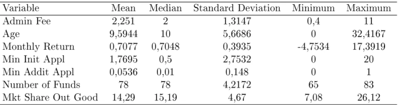
hundred, respectively. Table 1 presents some descriptive statistics of the variables considered. The age of a fund (Age) is defined as the number of months of existence divided by 12, minimum initial application (Min Init Appl) and minimum additional application (Min Addit Appl) are measured in tens of thousands of BRL.
Table 1: Descriptive Statistics
Variable Mean Median Standard Deviation Minimum Maximum
Admin Fee 2,251 2 1,3147 0,4 11
Age 9,5944 10 5,6686 0 32,4167
Monthly Return 0,7077 0,7048 0,3935 -4,7534 17,3919
Min Init Appl 1,7695 0,5 2,7532 0 20
Min Addit Appl 0,0536 0,01 0,148 0 1
Number of Funds 78 78 4,2172 65 83
Mkt Share Out Good 14,29 15,19 4,67 7,08 26,12
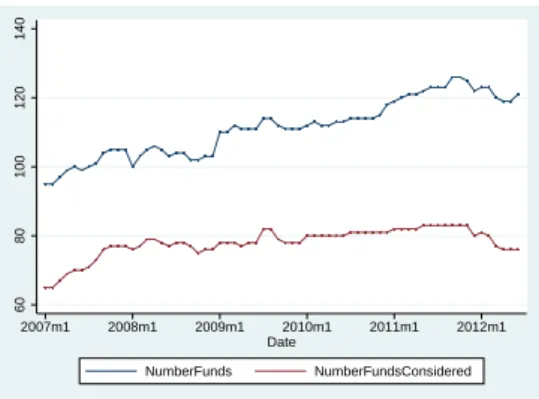
The graphics below show the evolution of net asset and number of funds considering all the funds existing and only those from the institutions considered.
To generate differences in preferences across individuals, we utilized a vector of shocks from a multivariate normal distribution𝒩(0𝐾, 𝐼𝐾) and two demographic variables. The
demograph-ics were sampled23 from National Household Sample Survey24 for each year, except for 2012
which has not data available yet and so the same data from 2011 were utilized. The number of simulations 𝑛𝑠 for each month is 100.
The variable sampled is the total income a person (with or more than 10 years old) received.25
The first variable is thelog(·)of the original variable then adjusted to have mean zero, while the
second is the original variable just adjusted to have mean zero and variance one.
21In August 2006 there was a reclassification, to avoid put in the sample funds that are now into another
category the selected data starts in 2007.
22These are Santander, Banco do Brasil, Bradesco, Caixa, HSBC, Itaú Unibanco. 23The different weight for each stratum were considered.
24In portuguese: Pesquisa Nacional por Amostra de Domicílios (PNAD).
5.00e+10
5.50e+10
6.00e+10
6.50e+10
7.00e+10
2007m1 2008m1 2009m1 2010m1 2011m1 2012m1 Date
TotalNetAsset ConsideredNetAsset
Figure 1: Total Net Asset
60
80
100
120
140
2007m1 2008m1 2009m1 2010m1 2011m1 2012m1 Date
NumberFunds NumberFundsConsidered
Figure 2: Number of Funds
Lastly, the market size was defined as the maximum monthly total net asset in the period considered of the fixed income funds that has the characteristics cited above, except being offered by the largest commercial banks. Thus the outside good represents both the substitution for another categories of funds or investment and to funds offered from institutions not considered.26
7.3 Results
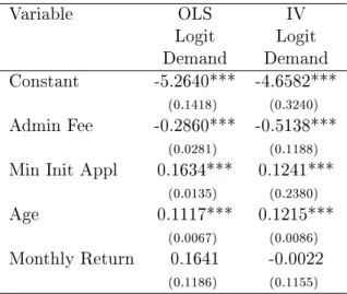
Now we will report the results for specifications of demand and supply presented. In Table2
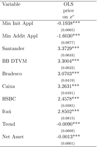
are those for Logit demand specification not considering and considering the correlation between prices and unobserved product characteristics. These are referred as OLS Logit demand and IV Logit demand, respectively. A model of supply assuming marginal cost pricing is presented in Table3 with a regression of price in the cost shifters𝑥𝑐.
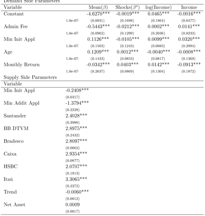
The results from joint estimation of demand and supply supposing a RC-Logit for demand and supply considered in Supply Section are presented in Table4. For demand the first column presents the values of mean coefficients𝛼 and𝛽, the second are the𝛽𝑠 which captures the effect
of shocks in each observable characteristic, while the third and fourth columns are the𝛽𝑑 which
represents the effects of demographics in the observable characteristics.
In both specifications presented in Table2 all parameters are significant except for Monthly Return.27 The Age of a Fund has the positive expected sign. Minimum Initial Application
(Min Init Appl) is measured in tens of thousands ans has positive sign. The Administration Fee (Admin Fee) also has the expected sign in both models and correcting for endogeneity has its absolute value raised. This makes sense since it is supposed that this variable is positively correlated with the unobserved error term𝜉so when its effect is isolated its value is supposed to
increase in modulus.
For supply side considered isolatedly Table 3 presents the results. Minimum Initial Appli-cation (Min Inic Appl) and Minimum Additional AppliAppli-cation (Min Addit Appl) are measured in tens of thousands and have negative sign, indicating that an increase in these variables lower the costs. Six dummy variables, one for each institution are included. A Trend (measured in months) although statistically significant does not seems to be economically significant. The Net Asset (in tens of millions) are significant and its negativeness indicates the presence of increasing returns to scale.
26The market share of the outside good ranges from 7.08% to 26.12%.
Table 2: Results from Logit Demand
Variable OLS IV
Logit Logit
Demand Demand
Constant -5.2640*** -4.6582***
(0.1418) (0.3240)
Admin Fee -0.2860*** -0.5138***
(0.0281) (0.1188)
Min Init Appl 0.1634*** 0.1241***
(0.0135) (0.2380)
Age 0.1117*** 0.1215***
(0.0067) (0.0086)
Monthly Return 0.1641 -0.0022
(0.1186) (0.1155)
Standard Errors are reported in parentheses *** means that variable is significant at 1% level
Finally Table4presents the results from joint estimation of demand and supply, being all the parameters significant except for the Net Asset. The sign of the mean coefficients for demand𝛼
and 𝛽 has the same sign from the estimation presented in Table2.
Administration Fee (Admin Fee) has the expected negative sign of the mean coefficient. The large coefficient for the 𝛽𝑠
𝐴𝑑𝑚𝑖𝑛𝐹 𝑒𝑒 shows a wide variation in the willingness to pay, while the
positive sign from the coefficients from the interaction with income, indicates that persons with more income are less sensitive to the Administration Fee. Minimum Initial Application (Min Init Appl) has positive sign as well as Age, which indicates that this kind of market could present a reputation effect such that a person would prefer funds with longer existence and/or good performance tends to maintain the funds while the opposite may be closed. Differently than expected, the mean effect of the Monthly Return is negative.28
For the supply side, all parameters have the same sign as in the previous estimation, except for the Net Asset which is positive but not significant.29
28For a month the return utilized is from the previous month, since the return of a month is only know in the
next.
Table 3: Results from Marginal Cost Pricing
Variable OLS
price on 𝑥𝑐
Min Init Appl -0.1938***
(0.0065)
Min Addit Appl -1.6030***
(0.0877)
Santander 3.3729***
(0.0633)
BB DTVM 3.3004***
(0.0622)
Bradesco 3.0703***
(0.0419)
Caixa 3.2631***
(0.0491)
HSBC 2.4578***
(0.0385)
Itaú 2.8502***
(0.0815)
Trend -0.0090***
(0.0008)
Net Asset -0.0013***
(0.0001)
Table 4: Results from Demand and Supply Side in RC-Logit
Demand Side Parameters
Variable Mean(𝛽) Shocks(𝛽𝑠) log(Income) Income
Constant -4.6270*** -0.0019*** 0.0465*** -0.0016***
1.0e-07· (0.0031) (0.1698) (0.1864) (0.0477)
Admin Fee -0.5443*** -0.0212*** 0.0002*** 0.0141***
1.0e-07· (0.0962) (0.1299) (0.2036) (0.0233)
Min Init Appl 0.1126*** -0.0105*** 0.0099*** 0.0320***
1.0e-07· (0.1503) (0.1243) (0.0083) (0.2994)
Age 0.1209*** 0.0012*** -0.0040*** -0.0008***
1.0e-07· (0.1433) (0.0853) (0.0817) (0.1369)
Monthly Return -0.0342*** 0.0403*** 0.0142*** -0.0913***
1.0e-07· (0.2637) (0.0869) (0.1304) (0.1872)
Supply Side Parameters Variable
Min Init Appl -0.2408***
(0.0317)
Min Addit Appl -1.3794***
(0.2228)
Santander 2.4028***
(0.3986)
BB DTVM 2.8975***
(0.2432)
Bradesco 2.8097***
(0.0662)
Caixa 2.9354***
(0.0877)
HSBC 2.0707***
(0.1813)
Itaú 3.3065***
(0.2272)
Trend -0.0060***
(0.0012)
Net Asset 0.0009
(0.0017)
Standard Errors are reported in parentheses *** means that variable is significant at 1% level
8 Conclusion
This dissertation presented models utilized to understand static models of demand in differ-entiated products markets. As well as examples of papers in main journals that utilizes RC-Logit to understand some features of determined market. Some limitations and challenges of these he-donic models of demand were discussed, even as with the supply side and the computational procedure. Finally was made an application to the Brazilian fixed income fund market.
Ackerberg et al.(2007) and some example of this procedure is atHendel and Nevo(2006). The next step for research is to focus on some feature of this market. Though not described in the data subsection, there is a negative correlation between Administration Fee and Miniminum Initial and Additional Application. Althought the results indicates that these last two variables lower costs, it is now known if the increase in the Administration Fee is justified only by an increase in costs or could be thought as a evidence of second degree price discrimination.30
Furthermore, this market (as well as many others that were analyzed utilizing static models) has a strong dynamic aspect, then using a dynamic model (if the data available permits) allows the study of more characteristics of this market. This too could be of interest for future research.
30Cohen (2008) made this analysis for the paper towel market utilizing data for sixty-four cities during eight
Bibliography
Ackerberg, D., Lanier Benkard, C., Berry, S., and Pakes, A. (2007). Econometric tools for ana-lyzing market outcomes. In Heckman, J. and Leamer, E., editors, Handbook of Econometrics, volume 6 of Handbook of Econometrics, chapter 63. Elsevier.
Berry, S., Levinsohn, J., and Pakes, A. (1995). Automobile prices in market equilibrium. Econo-metrica, 63(4):841–90.
Berry, S., Levinsohn, J., and Pakes, A. (2004a). Differentiated products demand systems from a combination of micro and macro data: The new car market. Journal of Political Economy, 112(1):68–105.
Berry, S., Linton, O. B., and Pakes, A. (2004b). Limit theorems for estimating the parameters of differentiated product demand systems. Review of Economic Studies, 71:613–654.
Berry, S. T. (1994). Estimating discrete-choice models of product differentiation. RAND Journal of Economics, 25(2):242–262.
Bresnahan, T. F. (1987). Competition and collusion in the american automobile industry: The 1955 price war. Journal of Industrial Economics, 35(4):457–82.
Chamberlain, G. (1987). Asymptotic efficiency in estimation with conditional moment restric-tions. Journal of Econometrics, 34(3):305–334.
Cohen, A. (2008). Package size and price discrimination in the paper towel market. International Journal of Industrial Organization, 26(2):502–516.
Dubé, J., Fox, J. T., and Su, C. (2012). Improving the numerical performance of static and dynamic aggregate discrete choice random coefficients demand estimation. Econometrica, 80(5):2231–2267.
Hendel, I. and Nevo, A. (2006). Measuring the implications of sales and consumer inventory behavior. Econometrica, 74(6):1637–1673.
Knittel, C. R. and Metaxoglou, K. (2012). Estimation of random coefficient demand models: Two empiricists’ perspective. The Review of Economics and Statistics, forthcoming.
Lee, J. (2011). A new computational algorithm for random coefficients model with aggregate-level data. Asian Meeting of the Econometric Society.
Levinsohn, J., Berry, S., and Pakes, A. (1999). Voluntary export restraints on automobiles: Evaluating a trade policy. American Economic Review, 89(3):400–430.
McFadden, D. L. (1974). Frontiers in Econometrics, chapter Conditional Logit Analysis of Qualitative Choice Behavior. Academic Press: New York.
Nevo, A. (2000a). Mergers with differentiated products: The case of the ready-to-eat cereal industry. RAND Journal of Economics, 31(3):395–421.
Nevo, A. (2000b). A practitioner’s guide to estimation of random-coefficients logit models of demand. Journal of Economics & Management Strategy, 9(4):513–548.
Nevo, A. (2001). Measuring market power in the ready-to-eat cereal industry. Econometrica, 69(2):307–42.
Rust, J. (1987). Optimal replacement of gmc bus engines: An empirical model of harold zurcher. Econometrica, 55(5):999–1033.
Stokey, N. L., Lucas, R. E., and Prescott, E. C. (1989). Recursive Methods in Economic Dynam-ics. Harvard University Press.
Appendix
1 clear all
2 load RF
3
4 global invIV ns x1 x2 s2_2 xs s_jt IV vfull dfull theta1 theti thetj cdid ...
cdindex cdid_u cdindex_u clean theta1_2 dum_inst IVd price
5
6 n_1=size(num,1);
7 dum_inst= num(: , [54 58 69 63 65 67]);
8
9 dum_ff= dummyvar(num(:,44));
10 dum_ff= dum_ff(:,2:3);
11
12 x1= [ones(n_1,1) num(:,31) num(:,27)/10000 num(:,34)/12 num(:,21)];
13 x2= [ones(n_1,1) num(:,31) num(:,27)/10000 num(:,34)/12 num(:,21)];
14
15 xs= [ num(:,27)/10000 num(:,35)/10000 dum_inst(:,[1 2 3 4 5 6 ]) num(:,1)];
16
17 s2_2=size(x2,2);
18
19 a=¬any(isnan(x1),2);
20 b=¬any(isnan(xs),2);
21
22 a1=(num(:,41)==0);
23 a2=(num(:,42)==0);
24 a3=(sum(dum_inst')'==1);
25 clean=and(a,b);
26 clean=and(a1,clean);
27 clean=and(a2,clean);
28 clean=and(a3,clean);
29
30 cdid_u=num(clean,1);
31
32 cdindex_u= [diff(cdid_u(:,1));1].*cumsum(ones(size(cdid_u,1),1));
33 cdindex_u(cdindex_u==0)=[];
34
35 ns = 100;
36 nmkt = 66;
37 nbrn = 174;
38
39 cdid = kron([1:nmkt]',ones(nbrn,1));
40 cdindex = [nbrn:nbrn:nbrn*nmkt]';
41
42 ivblp
43
44 % v=zeros(nmkt,size(x1,2)*ns);
45 % for i=1:ns;
46 % v(:,i:ns:size(x1,2)*ns) = mvnrnd(zeros(1,size(x1,2)),eye(size(x1,2)),nmkt);
47 % end
48
49 vfull = v(cdid_u,:);
50 dfull = demogr(cdid_u,:);
51
52 theta2w =[−0.00190000000000000 0.0465000000000000 −0.00160000000000000;
53 −0.0212000000000000 0.000200000000000000 0.0141000000000000;
54 −0.0105000000000000 0.00990000000000000 0.0320000000000000;
55 0.00120000000000000 −0.00400000000000000 −0.000800000000000000;
56 0.0403000000000000 0.0142000000000000 −0.0913000000000000];
59 [theti, thetj, theta2]=find(theta2w);
60
61 horz=[' mean sigma dem1 dem2 dem3'];
62
63 verti=['Constante ' ;
64 'taxa_adm ';
65 'AI_(10^6) ';
66 'Idade(anos)' ;
67 'Rentmes '];
68
69 pl=num(:,32);
70 pl(isnan(pl))=0;
71
72 temp = cumsum(pl);
73 sum1 = temp(cdindex,:);
74 sum1(2:size(sum1,1),:) = diff(sum1);
75 76 pl_max=max(sum1); 77 78 s_jt=pl./(pl_max); 79 80 pl(a3==0)=0;
81 temp1 = cumsum(pl);
82 sum2 = temp1(cdindex,:);
83 sum2(2:size(sum2,1),:) = diff(sum2);
84 sum_ms=sum2;
85
86 outshr= 1−(sum_ms(cdid,:)./(pl_max*ones(n_1,1)));
87
88 clear temp temp1 sum1 sum2
89
90 xs=[xs num(:,32)/10000000];
91 92 s_jt=s_jt(clean,:); 93 outshr=outshr(clean,:); 94 95 x1=x1(clean,:); 96 x2=x2(clean,:); 97 xs=xs(clean,:); 98 dum_inst=dum_inst(clean,:); 99 100 invIV=inv([IV'*IV]); 101
102 y = log(s_jt) − log(outshr);
103
104 invIVd=inv(IVd'*IVd);
105 mid = x1'*IVd*invIVd*IVd';
106 tiv = inv(mid*x1)*mid*y;
107 mvalold = x1*tiv;
108
109 et=y−mvalold;
110 111 temp1=x1'*IVd*invIVd*IVd'; 112 tesx=(et*et').*eye(size(x1,1)); 113 114 cov_t=inv(temp1*x1)*temp1*tesx*temp1'*inv(temp1*x1); 115
116 clear temp1
117
118 seiv=sqrt(diag(cov_t));
119 zstat=tiv./seiv;
120 pvalueiv=2*(1−normcdf(abs(zstat)));
122 theta1_2= tiv(2);
123 mvalold = exp(mvalold);
124 oldt2 = zeros(size(theta2));
125
126 t1 = inv(x1'*x1)*x1'*y;
127 mvalold1 = x1*t1;
128
129 et1=y−mvalold1;
130 tes1= x1*inv(x1'*x1);
131 tes11=(et1*et1').*eye(size(x1,1));
132 cov_t1= tes1'*(tes11)*tes1;
133
134 se1=sqrt(diag(cov_t1));
135 zstat1=t1./se1;
136 pvalue1=2*(1−normcdf(abs(zstat1)));
137 tx_fixa = num(clean,31);
138 ts=inv(xs'*xs)*xs'*tx_fixa;
139 mvalolds = xs*ts;
140
141 ets=tx_fixa−mvalolds;
142 tes2= xs*inv(xs'*xs);
143 tes22=(ets*ets').*eye(size(xs,1));
144
145 cov_ts= tes2'*(tes22)*tes2;
146 ses=sqrt(diag(cov_ts));
147 zstats=ts./ses;
148 pvalues=2*(1−normcdf(abs(zstats)));
149
150 price=num(clean,31);
151
152 save mvalold mvalold oldt2 theta1_2
153 clear oldt2 mvalold temp sum1
154 155 tic
156
157 options = optimset('GradObj','on','TolX',1.e−12,'TolFun',1.e−11,'MaxIter',100,...
158 'MaxFunEvals',100000);
159
160 [theta2,fval,exitflag,output] = fminsearch('objfun2',theta2, options);
161
162 comp_t = toc/60;
163
164 vcov = var_cov(theta2);
165 se = sqrt(diag(vcov));
166
167 tstat= [theta1(1:5); theta2]./se;
168 pvalue=2*(1−normcdf(abs(tstat)));
169
170 theta2w = full(sparse(theti,thetj,theta2));
171 t = size(se,1) − size(theta2,1);
172 se2w = full(sparse(theti,thetj,se(t+1:size(se,1))));
173 pvalue2w = full(sparse(theti,thetj,pvalue(t+1:size(pvalue,1))));
174 175
176 diary results
177 disp(horz)
178 disp(' ')
179 for i=1:size(x1,2)
180 disp(verti(i,:))
181 disp([theta1(i) theta2w(i,:)])
182 disp([se(i) se2w(i,:)])
183 disp([pvalue(i) pvalue2w(i,:)])
185
186 X = blkdiag(x1,xs);
187 load gmmresid
188 temp4=X'*IV*invIV*IV';
189 tesx=(gmmresid*gmmresid').*eye(size(X,1));
190
191 cov_t1t2=inv(temp4*X)*temp4*tesx*temp4'*inv(temp4*X);
192 sem = sqrt(diag(cov_t1t2));
193 194
195 tstat1= theta1./sem;
196
197 pvaluem=2*(1−normcdf(abs(tstat1)));
198
199 disp('[blp oferta]');
200 disp(' vmai vmaa sant bb brad caixa hsbc ...
itau')
201 x = [theta1(size(x1,2)+1:length(theta1))]';
202 y = [sem(size(x1,2)+1:length(theta1))]';
203 z = [pvaluem(size(x1,2)+1:length(theta1))]';
204 disp(x)
205 disp(y)
206 disp(z)
207
208 disp('[IV logit demanda]');
209 disp(' Constante taxa_adm AI_(10^60) Idade(anos) Rentmes')
210 x = [tiv seiv pvalueiv]';
211 disp(x)
212
213 disp('[OLS logit demanda]');
214 disp(' Constante taxa_adm AI_(10^60) Idade(anos) Rentmes')
215 x = [t1 se1 pvalue1]';
216 disp(x)
217
218 disp('[ols oferta]');
219 disp(' vmai vmaa sant bb brad caixa hsbc itau')
220 x = [ts ses pvalues]';
221 disp(x)
222 223 224
225 disp(['GMM objective: ' num2str(fval)])
226 disp(['# of objective function evaluations: ' num2str(options(10))])
227 disp(['run time (minutes): ' num2str(comp_t)])
228 diary off
1 function [f] = objfun2(theta2)
2 global invIV theta1 theti thetj x1 xs IV s_jt theta1_2
3
4 theta2w = full(sparse(theti,thetj,theta2));
5
6 ∆ = meanval(theta2);
7
8 ∆s = pri_m(theta1_2,theta2w);
9
10 Y = [∆ ; ∆s];
11
12 if max(isnan(Y)) == 1
13 f = 1e+10
14 else 15
17
18 temp1 = X'*IV;
19 temp2 = Y'*IV;
20
21 theta1 = inv(temp1*invIV*temp1')*temp1*invIV*temp2';
22 gmmresid = Y − X*theta1;
23 temp3 = gmmresid'*IV;
24
25 f = temp3*invIV*temp3';
26
27 clear temp1 temp2 temp3
28
29 theta1_2
30 theta2
31 theta1(2)
32
33 theta1_2=theta1(2)
34 35
36 clear temp1
37
38 if nargout>1
39 load mvalold
40
41 end
42 end 43
44 disp(['GMM objective: ' num2str(f)])
45
46 save gmmresid;
1 function f = meanval(theta2)
2 global theti thetj silent x2 s_jt
3 load mvalold.mat
4
5 if max(max(abs(theta2−oldt2)) < 0.01)
6 tol = 1e−9;
7 flag = 0;
8 else
9 tol = 1e−6;
10 flag = 1;
11 end 12
13 theta2w = full(sparse(theti,thetj,theta2));
14 expmu = exp(mufunc(x2,theta2w));
15 save expmu expmu
16 norm = 1;
17 avgnorm = 1;
18
19 i = 0;
20 while norm > tol*10^(flag*floor(i/50)) & avgnorm > 1e−3*tol*10^(flag*floor(i/50))
21
22 mval = mvalold.*s_jt./mktsh(mvalold,expmu);
23
24 t = abs(mval−mvalold);
25 norm = max(t);
26 avgnorm = mean(t);
27 mvalold = mval;
28 i = i + 1;
29 end
30 disp(['# of iterations for ∆ convergence: ' num2str(i)])
32 if flag == 1 & max(isnan(mval)) < 1;
33 mvalold = mval;
34 oldt2 = theta2;
35 save mvalold.mat mvalold oldt2
36 end
37 f = log(mval);
1 function f = pri_m(theta1_2,theta2w)
2 global ns vfull dfull s2_2 st2_2 cdindex_u dum_inst x2 price s_jt
3
4 load denom
5 load mvalold.mat mvalold
6
7 [theti, thetj, theta2]=find(theta2w);
8
9 ind_pan=[ 0 cdindex_u'];
10
11 expmu = exp(mufunc(x2,theta2w));
12 expmval= mvalold;
13
14 eg = expmu.*kron(ones(1,ns),expmval);
15
16 for k = 1:66;
17
18 k_min =ind_pan(k)+1;
19 k_max=ind_pan(k+1);
20 kM=k_max−k_min+1;
21
22 a_linha=zeros(kM,20);
23 B=zeros(kM,20);
24 D=zeros(kM,kM,ns);
25 26
27 for i = 1:20;
28
29 v_i = vfull(:,i:ns:s2_2*ns);
30 d_i = dfull(:,i:ns:(st2_2−1)*ns);
31 32
33 a_linha(k_min:k_max,i)= eg(k_min:k_max,i) .*( theta1_2*ones(kM,1) + ...
v_i(k_min:k_max,2)*theta2w(2,1) + (d_i(k_min:k_max,:)*theta2w(2,2:st2_2)'));
34
35 B(k_min:k_max,i)= denom(k_min:k_max,i);
36 37
38 D(:,:,i) = ((1./(B(k_min:k_max,i).^2))*ones(1,kM)) .* ...
(−eg(k_min:k_max,i)*a_linha(k_min:k_max,i)'+ ...
diag(a_linha(k_min:k_max,i).*B(k_min:k_max,i)) );
39 end
40
41 D = sum(D,3)/ns;
42
43 D=D';
44 DI= dum_inst(k_min:k_max,:)*dum_inst(k_min:k_max,:)';
45
46 pri_m(k_min:k_max,1)=price(k_min:k_max) − (D.*DI)\s_jt(k_min:k_max);
47
48 clear a_linha B D DI
49 50 end 51
1 function f = ind_sh(expmval,expmu)
2 global ns cdindex_u cdid_u
3 eg = expmu.*kron(ones(1,ns),expmval);
4 temp = cumsum(eg);
5
6 sum1 = temp(cdindex_u,:);
7 sum1(2:size(sum1,1),:) = diff(sum1);
8
9 denom1 = 1./(1+sum1);
10 denom = denom1(cdid_u,:);
11
12 save denom denom
13 f = eg.*denom;
1 function f = mktsh(mval, expmu)
2 global ns
3 f = sum((ind_sh(mval,expmu))')/ns;
4 f = f';
1 function f = mufunc(x2,theta2w)
2 global ns vfull dfull cdid_u
3
4 st2_2=size(theta2w,2);
5 s2_2=size(x2,2);
6
7 mu = zeros(size(cdid_u,1),ns);
8 for i = 1:ns
9 v_i = vfull(:,i:ns:s2_2*ns);
10 d_i = dfull(:,i:ns:(st2_2−1)*ns);
11 mu(:,i) = ...
(x2.*v_i*theta2w(:,1))+x2.*(d_i*theta2w(:,2:st2_2)')*ones(s2_2,1);
12 end
13 f = mu;
1 function f = var_cov(theta2)
2 global IVd
3
4 load mvalold
5 load gmmresid
6
7 N = size(x1,1);
8 gmmresid=gmmresid(1:N);
9
10 Z = size(IVd,2);
11 temp = jacob(mvalold,theta2);
12 A=IVd'*[−x1 temp];
13
14 temp2= IVd'*gmmresid ;
15 vco = 1/N*(temp2*temp2');
16
17 vco = (vco+vco')/2;
18
19 vco=inv(vco);
20