General Regression and Representation
Model for Classification
Jianjun Qian1, Jian Yang1*, Yong Xu2
1.School of Computer Science and Engineering, Nanjing University of Science and Technology, Nanjing, 210094, China,2.Bio-Computing Research Center, Shenzhen Graduate School, Harbin Institute of Technology, Shenzhen, 518055, China
Abstract
Recently, the regularized coding-based classification methods (e.g. SRC and CRC) show a great potential for pattern classification. However, most existing coding methods assume that the representation residuals are uncorrelated. In real-world applications, this assumption does not hold. In this paper, we take account of the correlations of the representation residuals and develop a general regression and representation model (GRR) for classification. GRR not only has advantages of CRC, but also takes full use of the prior information (e.g. the correlations between representation residuals and representation coefficients) and the specific
information (weight matrix of image pixels) to enhance the classification
performance. GRR uses the generalized Tikhonov regularization and K Nearest Neighbors to learn the prior information from the training data. Meanwhile, the specific information is obtained by using an iterative algorithm to update the feature (or image pixel) weights of the test sample. With the proposed model as a platform, we design two classifiers: basic general regression and representation classifier (B-GRR) and robust general regression and representation classifier (R-(B-GRR). The experimental results demonstrate the performance advantages of proposed methods over state-of-the-art algorithms.
Introduction
As well known, the nearest neighbor classifier (NN) is one of the most popular classifiers due to its simplicity and efficiency. However, NN just uses one training sample to represent test sample. To address this problem, the nearest feature line (NFL) uses two training samples of each class to represent test sample [1]. The nearest feature plane (NFP) applies three samples to represent test sample [2].
OPEN ACCESS
Citation:Qian J, Yang J, Xu Y (2014) General Regression and Representation Model for Classification. PLoS ONE 9(12): e115214. doi:10. 1371/journal.pone.0115214
Editor:Hong-Bin Shen, Shanghai Jiaotong University, China
Received:August 13, 2014
Accepted:November 18, 2014
Published:December 22, 2014
Copyright:ß2014 Qian et al. This is an open-access article distributed under the terms of the Creative Commons Attribution License, which permits unrestricted use, distribution, and repro-duction in any medium, provided the original author and source are credited.
Data Availability:The authors confirm that all data underlying the findings are fully available without restriction. All relevant data have been deposited to Figshare (http://dx.doi.org/10.6084/m9.figshare. 1248893).
Funding:This work was partially supported by the National Science Fund for Distinguished Young Scholars under Grant Nos. 61125305, 61472187, 61233011 and 61373063, the Key Project of Chinese Ministry of Education under Grant No. 313030, the 973 Program No. 2014CB349303, Fundamental Research Funds for the Central Universities No. 30920140121005, and Program for Changjiang Scholars and Innovative Research Team in University No. IRT13072. The funders had no role in study design, data collection and analysis or preparation of the manuscript.
Furthermore, some classifiers leverage more training samples for test sample representation, such as the local subspace classifier (LS) [3] and nearest subspace classifier (NS) [4,27], which represent the test sample via all training samples of each class. Actually, all these methods can be considered as variants of linear regression based methods. To prevent over-fitting, the L2-regularizer is generally
used in the linear regression model. In the past years, the L1-regularizer, which is
closely linked to sparse representation, becomes a hot theme in information theory, signal/image processing and related areas. Meanwhile, numerous findings of neuroscience and biology form a physiological base for sparse representation [5–7].
Recently, many efforts have been made to apply sparse representation methods to pattern classification tasks, including signal/image classification and face recognition etc. Labusch et al. presented a simple sparse-coding strategy for digit recognition and achieved state-of-the-art results on the MNIST benchmark [8]. Yang et al. addressed the problem of generating a super-resolution (SR) image from a single low-resolution input image via sparse representation [9]. Mairal et al. elaborated a framework for learning multi-scale sparse representations of images with applications to image denoising and inpainting [10]. Yang et al. employed sparse coding instead of vector quantization to capture the significant properties of local image descriptors for image classification [11]. Particularly, Wright et al. introduced a sparse representation based classification (SRC) and successfully applied it to identify human faces with varying illumination changes, occlusion and real disguise [12]. In their method, a test sample image is coded as a sparse linear combination of the training images, and then the classification is achieved by identifying which class yields the least residual. Theodorakopoulos et al. introduced a face recognition method based on sparse representation of facial image patches [37]. Subsequently, Gao et al. proposed Kernel Sparse Representation for image classification and face recognition. KSR actually is the sparse coding technique in a high dimensional feature space via some implicit feature mapping [39]. Yang and Zhang constructed a Gabor occlusion dictionary for SRC to reduce the computation cost by using Gabor feature [13].
Although the newly-emerging SRC shows great potential for pattern
classification, it lacks theoretical justification. Yang et al. provided an insight into SRC and analyzed the role of L1-optimizer [14]. They think that L1-optimizer
contains two properties: sparsity and closeness. However, L0-optimizer can only
represented by CESR and RSC for error detection, He et al. [38] built a half-quadratic framework by defining different half-half-quadratic functions. The frame-work enables to perform both error correction and error detection. Furthermore, He et al. also leverage the half-quadratic framework to address the feature selection and subspace clustering problems [48,49]. In addition, Zhou et al. incorporated the Markov Random Field model into the sparse representation framework for spatial continuity of the occlusion [40]. Li et al. explored the intrinsic structure of continuous occlusion and proposed the structured sparse error coding (SSEC) model [41]. Ou et al. proposed a novel structured occlusion dictionary learning method for robust face recognition [42]. Apart from these methods, many related tasks have been reported [18–20,32–35].
With the widely use of sparse representation for classification, some scholars question the role of sparseness for image classification [21,22]. Zhang et al. analyzed the working principle of SRC and believed that it is the collaborative representation that improves the image classification accuracy rather than the L1
-norm sparsity. Consequently, Zhang et al. presented a collaborative representation based classification with regularized least square (CRC) [23]. Compared with SRC, CRC delivers very competitive classification results with little computation time. Subsequently, Yang et al. proposed a relaxed collaborative representation model (RCR) which effectively captures the similarity and distinctiveness of different features for pattern classification [24]. Theodorakopoulos et al. gave a collaborative sparse representation model in dissimilarity space for visual classification tasks [43].
Most of previous works assume that representation residuals are mutually uncorrelated [31]. It’s difficult to hold this assumption in real-world applications. Actually, it is common to have data where representation residuals are correlated. Thus, in this paper, we consider to eliminate the correlations between
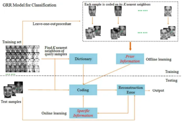
representation residuals and present a novel model named General Regression and Representation (GRR) for pattern classification. GRR mainly aims to take account of the prior information (e.g. the correlations between representation residuals and representation coefficients) and the specific information (weight matrix for each image pixel) so as to enhance the classification performance under different conditions. Specifically, GRR selects one image from training set and finds its K nearest neighbors in rest ones to code the image. In this way, all the training images can be coded on its K nearest neighbors. Subsequently, we calculate the correlations between representation residuals and representation coefficients by virtue of the reconstruction error and representation coefficient of each training image. For each test sample, we apply the iterative algorithm to achieve the weight of each image pixel. The overview of GRR is shown in Fig. 1. Compared with other regression based classification methods, the novelty of the proposed model is threefold:
N
Second, GRR captures the prior information from the training set via the generalized Tikhonov regularization in conjunction with the K Nearest Neighbor method and leaving-one-out procedure;N
Third, with the GRR model as a platform, we design two classifiers: Basic GRR (B-GRR) and Robust GRR (R-GRR) by combining the prior information and the specific information with different strategies.To evaluate the proposed model, we finally use four databases which involve different recognition tasks: the CENPARMI dataset for handwritten numerical recognition, the NUST603 dataset for handwritten Chinese character recognition, the AR dataset for face recognition and face occlusion recognition, and the Extended Yale B dataset for face recognition with extreme lighting changes and face recognition with random block occlusion. Experimental results demonstrate the effectiveness of the proposed model.
This paper is the extended version of our conference paper [36]. In this paper, we provide a more in-depth analysis and more extensive experiments on the proposed model.
Fig. 1. An overview of General Regression and Representation model for classification.
Current Methods and Their Problems
A. Current Methods
Suppose there are c known pattern classes. Let Ai be the matrix formed by the training samples of Class i, i.e.,Ai~½yi1,yi2, ,yiMi[RN
|Mi
, where Mi is the number of training samples of Class i. Let us define a matrix
A~½A1,A2, ,Ac[RN|M, whereM~Pc
i~1Mi. The matrix A is obviously
composed of entire training samples.
Sparse Representation based Classification
Given a test sample y, we present y in a over-complete dictionary whose basis vectors are training samples themselves. i.e., y5Ax. The sparse solution toy5Ax can be sought by solving the follow optimization problem:
^
x~arg mink kx
0 s:t: Ax~y, ð1Þ
However, solving theL0optimization is NP hard problem. Fortunately, recent
researches reveal that L0 optimization and L1 optimization are equivalent when the solution is sparse enough. In general, the sparse representation problem can be formulated as:
^
x~arg mink kx
1 s:t: Ax~y: ð2Þ
The problem is equivalent to^x~arg min
x ky-Axk 2
2zlk kx 1.
Then classification rule is:
identif y(y)~arg min
i fr(yi)g ð3Þ
where ri(y)~jjy{^yijj2~jjy{Adi(^x)jj2, di(^x)is the nonzero coefficient vector associated with class i.
Correntropy-based Sparse Representation
Correntropy-based Sparse Representation (CESR) leverages the maximum correntropy criterion to design the classifier for robust face recognition [17]. Similar with SRC, CESR aims to reconstruct a test sampleyusing existing training samples as well as possible. The correntropy-based sparse model is formulated as:
^
x~arg max
x
XN
j~1
g(yj{X c
i~1
Aijxi){lX c
i~1
xi, s:t: xiw0 ð4Þ
where g(x)~exp({x
2
s2 )is a gaussian kernel function. The above nonlinear
identif y(y)~arg max
i fc(yi)g ð5Þ
where c(yi)~g(y-^y
i)~g(y-Adi(^x)) ands2~
1
2cky{Aidi(^x)k
2 2.
Robust Sparse Representation
The robust sparse representation problem can be reformulated as the following minimization problem:
^
x~arg min
x
XN
j~1
w((y-Ax)j)zlk kx 1, ð6Þ
where w(:)is a robust M-estimator and can be optimized by half-quadratic (HQ) optimization,(:)jmeans thej-th dimension of input data. In HQ framework, RSR problem can be considered as an iterative regularization problem and applying a number of unconstrained quadratic problems to solve the optimization problem. The classification rule is
identif y(y)~arg min
i fw(y-Adi(^x))g ð7Þ
CRC with Regularized Least Square
CRC uses the regularized least square method to represent test sample can lead the similar results to L1-norm regularization but with low computation burden. The
model is formulated as:
^
x~arg min
x ky-Axk 2
2zlk kx 2
2 ð8Þ
where lis the regularization parameter. The regularization term can help us to achieve a stable solution. Meanwhile, it also introduces a little sparse constraint to
the ^x, which is much weaker than SRC. The solution of CRC in (8) with
regularized least square as follows:
^
x~(AATzlI)-1ATy ð9Þ
The classification rule of CRC is similar with SRC. However, ri(y)~jjy{Adi(^x)jj
2=jjdi(^x)jj2. We classifyyby checking the reconstruction error
of each class to yield the classification result.
Linear Regression Classification
^
xi~arg min
xi jjy-Aixijj 2
2 ð10Þ
The solution of^xi is:
^
xi~(AiAiT)-1AiTy ð11Þ
LRC is made in favor of the class with the minimum distancedi(y)~ y{^y i
2.
B. Problems
The most previous works, including RSC, SRC, CRC, CESR et al, assume that the representation residuals are homoskedastic and mutually uncorrelated. In real-world applications, these assumptions do not hold. In particular, when the elements of representation residuals have unequal variances and are correlated, variance of representation residuals is no longer a scalar variance-covariance matrix, and hence there is no guarantee that the least square estimator is the most efficient within the class of linear unbiased estimators [46,47]. Here, we also give an example to demonstrate this view. Fig. 2 shows the example, where 200 samples of each class are selected from the CENPARMI dataset, each sample is coded on its top 200 neighbors from the rest samples. The correlation matrix map of representation residuals is shown in Fig. 2, from which we can see that these representation residuals are actually correlated.
General Regression and Representation Model for
Classification (GRR)
This section mainly introduces two classifiers: Basic GRR and Robust GRR, which designed with the GRR model as a platform. Basic GRR is built to address the correlation problem of representation residuals in other regression models. Robust GRR is an extended version of the basic GRR model, which provides a mechanism to deal with noises in test samples.
A. Basic GRR
Let A be the matrix formed by the K nearest neighbors of the test sample from training set, M be the number of training samples, and ybe the test sample. Our model is
^
x~arg min
x ky-Axk
2
Pzk kx
2
Q ð12Þ
We call above model as the basic general regression and representation (B-GRR). Actually, this model can be reformulated as follows:
^
x~arg min
x (y-Ax)
T
P(y-Ax)zxTQx ð13Þ
IfP and Qare known, from the generalized Tikhonov regularization [30,44], we know there is a close-form solution:
^
x~(ATPAzQ)-1ATPy ð14Þ
However, P andQ are unknown beforehand. We here employ a generative method to estimate these two correlation matrices PandQin the training stage. Basically, we assume the representation residual e~y-Ax and representation coefficient vector x satisfy multivariate normal distributions. Then, P can be estimated by using the inverse covariance matrix ofe[30,44]. To explain why the matrix P can be estimated in this way, we first letR be a non-stochastic
transformed matrix and ignore the regularization term for the moment. Eq. (11) can be reformulated as
^
x~arg min
x k(Ry)-(RA)xk
2
2 ð15Þ
whereRydenotes the transformed dependent variable andRAis the matrix of the transformed explanatory variables. It can be seen that RA also has full column rank provided that R is nonsingular. The solution is
^
x~(ATRTRA)-1ATRTRy ð16Þ
Fig. 2. An example shows partial correlation matrix (only select top 50 from 121 ones) of representation residuals.
Obviously, we can see thatP~RTR. The natural question then is how to find a transformation matrix that yields the most efficient estimator among all linear unbiased estimators. Generally speaking, one should chooseRas a non-stochastic and non-singular matrix like RTPeR~s2
eI. It should be note that
P
e is symmetric and positive definite so that it can be orthogonally diagonalized as CTPeC~L, whereCis the matrix of eigenvectors corresponding to the matrix of eigenvalues L. For P{1=2
e ~L
{1=2
CT, we have P{1=2
e
P
e(
P{1=2
e )
T~I. This
result suggests that the transformation matrix R should be proportional to
P{1=2
e . Given this choice ofR, we have P~
P{1
e .
The matrix Qcan be estimated by using the inverse covariance matrix of x
[30,45]. Q is introduced to generate a Mahalanbios distance based regularization term. The main difference between ridge regression and the proposed method is that ridge regression uses Euclidean distance to constrain the representation coefficients and the proposed method applies Mahalanbios distance to constrain them. It’s believed that Mahalanbios distance might provide a better regulariza-tion term than Euclidean distance since there exists correlaregulariza-tions between representation coefficients. Ideally, we should maximize the correlation of representation coefficients of the homo-class samples and minimize the correlation of representation coefficients of the hetero-class samples simulta-neously in the training process. However, it is difficult to model this because we have different numbers of representation coefficients corresponding to homo-class and hetero-homo-class samples. A feasible way is to eliminate the correlations of all representation coefficients. This leads to more significant effects on the
representation coefficients of hetero-class samples than on those of homo-class samples, since the representation coefficients of hetero-class samples are much more than those of the homo-class samples in multi-class classification problems.
Based on the above analysis, we give the details of estimating Pand Q as follows.
Lety(itrain)be thei-th sample of the training set.A(itrain) is the matrix formed by the K nearest neighbors ofy(itrain) from the training set. We set P05I andQ05I. The coding coefficient vector of y(itrain) onto A(itrain) is:
^
x(itrain)~arg min
x(itrain)
y(itrain)-A
(train)
i x
(train)
i 2 P0
z x(itrain)
2
Q0 ð17Þ
Letei~y(train)
i {A
(train)
i ^x
(train)
i and m1~M1
PM
i~1
ei. ThenP can be estimated by
P~(X
e
zl1I){1 ð18Þ
whereP
e~M1
PM
i~1
(ei{m
1)(ei{m1)T.l1is the regular parameter. Note thatl1Iis
Letm2~1
M
PM
i~1
x(itrain). Then, Qcan be estimated by
Q~(X
x
zl2I){1 ð19Þ
where P
x~M1
PM
i~1
(x(train)
i {m2)(x
(train)
i {m2)
T. l
2is the regular parameter and l2 I
is also used to avoid the singularity of the covariance matrix.
In the testing stage, for a given test sampley, we find its K nearest neighbors from the training set to form the matrixA. Then, we calculate the representation coefficients vector ^x using Eq. (14). We can reconstruct the test sampley as ^
yc~Adc(^x)by employing the representation coefficients associated withc-th class. The corresponding reconstruction error of c-th class is defined:
rc(y)~ky{Adc(^x)k2
dc(^x)
k k2 ð20Þ
The decision rule is: if rl(y)~min
c rc(y), yis assigned to Class l.
B-GRR makes full use of the prior information of the training set. It works well when the testing samples share the same probability distribution with the training samples. The algorithm of B-GRR for classification is summarized in Algorithm 1.
Algorithm 1
B-GRR for Classification
Input: Dictionary A, test sample y. Initial values P0 and Q0
1. Normalize the columns of A to have unit L2-norm.
2. The prior information matrices P and Q are learned from training set by using Eq. (18) and Eq. (19).
3. The test sample yis coded on its K nearest neighborsA via Eq. (12). 4. Compute the residuals of each class.
Output: y is assigned to the class which yields the minimum residuals.
B. Robust GRR
In image classification problems, illumination, expression or pose changes may cause significant differences between test samples and training samples. Therefore, it is necessary to introduce the test sample specific information to alleviate the effect caused by the differences between test samples and training samples. This specific information is to give a weight to each feature (or image pixel) of the sample, which can be learned online via the iteratively reweighted algorithm.
^
x~arg min
x W
1=2(y
-Ax)
2
Pzk kx
2
Q ð21Þ
IfP, Q andW are known, the above model can be solved explicitly using the formula:
^
x~½AT(W1=2)TP(W1=2)AzQ-1AT(W1=2)TP(W1=2)y ð22Þ
Since PandQ can be learned offline using the same method as in Basic GRR, the remaining problem is to learn the specific informationWonline. Specifically, given a test sampley, we firstly compute the representation residualseofyso as to
initialize the weight. The residual eis initialized as e5y-yini, and yiniis the initial
estimation of the true images from the observe samples. In this study, we simply set yinias the mean image of all samples in the coding dictionary since we don’t know which class the test imageybelongs to. With the initializedyini, our method can estimate the weight matrixWiteratively.Wactually is a diagonal matrix,Wk,k (i.e. vh(ek)) is the weight assigned to the k-th pixel of test image. The weight function [16] is:
vh(ek)~
exp(ab{a(ek)2)
1zexp(ab{a(ek)2) ð23Þ where aand b are positive scalars.
In addition, Eq. (22) is the explicit solution of Eq. (21). The process is terminated when the difference of the weights between adjacent iterations satisfies the following condition:
W(t){W(t{1)
2= W
(t{1)
2vc ð24Þ
The R-GRR algorithm for classification is summarized in Algorithm 2.
Algorithm 2
R-GRR for Classification
Input: Dictionary A, test sample y. Initial values P0, Q0 and yini.
1. Normalize the columns of A to have unit L2-norm, test sample y with L2
-norm and yt initialized as yini.
2. The prior information matricesPand Qare learned from the training set by using the generalized Tikhonov regularization and KNN.
3. The test sample yis coded on its K nearest neighborsA.
a. Compute residual e(t)~y{y(t)
b. Estimate weights vh(e(kt))~
exp(a(t)b(t)
{a(t)(e(kt))2)
1zexp(a(t)b(t){a(t)(e(kt))2) c. Code ^x~arg min
x (W
(t))1=2(
y-Ax)
2 P
zk kx 2
d. Compute the reconstructed test sample y(t)~Ax(t), and let t 5 t + 1 e. Go back to step a) until the maximal number of iterations is reached, or
convergence is met as shown in Eq. (24)
4. Compute the residuals of each class.
Output: y is assigned to the class which yields the minimum residuals.
C. Robust GRR for Occlusion Cases
In real-world image recognition tasks, occlusion is one of the most challenge problems. To overcome this problem, we combine advantages of the prior information Q and the specific information W to enhance the classification performance. As we know, P reflects the correlations between representation residuals. If there are great differences between the test sample and the training samples, the resulting reconstruction error does not follow the original
distribution. In this case, we cannot employ the matrix Pto eliminate the correlations between representation residuals of test images. So, the matrix P is removed from the model when there is occlusion, real-disguise or noises in test image. In contrast, the matrix Q won’t be affected whether the test image has occlusion or not since it is mainly used as a regularization term. Therefore, we keep matrix Qin the model, which can have positive effect on the performance. Then Eq. (19) can be reformulated as:
^
x~arg min
x W
1=2(y
-Ax)
2 2zk kx
2
Q ð25Þ
The solution of this model is:
^
x~(ATWAzQ)-1ATWy ð26Þ
Further Analysis of GRR
In this section, we will further analyze the role of P andQ in GRR. P is a symmetric matrix which is learned from the training set and can be decomposed into RTR, whereRis a non-singular transformed matrix and is used to eliminate the correlations between representation residuals. The matrix Q in the
residual criterion, we know that B-GRR, using the prior information contained in
PandQ, achieves the right result, while CRC fails without using this information. We then compare the obtained representation coefficients of CRC and B-GRR. Fig. 3 (b)shows the representation coefficients of CRC and B-GRR for the same test image as shown in Fig. 3 (a). The representation coefficients of the homo-class samples are highlighted in blue. CRC provides a very dense representation, while B-GRR gives a sparser representation due to the KNN based dictionary selection. In comparison with CRC, the representation coefficients of B-GRR seem to be more congregated on the homo-class samples.
We also give an example to compare our methods with some state-of-the-art methods on handing occlusions. In the example, two classes of face images from the AR database, as shown in Fig. 4, are used for training. We test two cases of real-world disguise images: the images with sunglasses and the images with scarves. In Fig. 5 (a)andFig. 5 (b), the left column contains the disguise images. In our test, we use R-GRR, RRC_L2, RSC, B-GRR, SRC and CRC to deal with
occlusion. For each occluded image, the reconstructed images (recovered clean image) and the residual images (recovered occlusion) are shown in Fig. 5. From Fig. 5, we can see that R-GRR achieves comparable result with RRC_L2, RSC and
significantly outperforms other methods. However, R-GRR is slightly better than RRC_L2 and RSC from the viewpoint of weight maps.
Fig. 3. The example shows the importance of P and Q for classification.(a) The classification result is right when our model B-GRR using the prior informationPandQ. However, we obtain the wrong result using CRC. (b) The corresponding representation coefficients of B-GRR and CRC.
Experiments
In this section, we perform experiments on four benchmark databases and compare the proposed model GRR with state-of-the-art models. Note that here in SRC and RSC, the matlab function ‘‘l1-ls’’ [25] is used to calculate the sparse representation coefficient. In the following experiments, the parameterais 8 and Fig. 4. Two classes of samples from the AR database.(a) Recovered clean image and occluded part via six methods for the image with sunglasses. For R-GRR, RRC_L2 and RSC, we also give the corresponding weight maps. (b) Recovered clean image and occluded part via six methods for the image with scarf. For R-GRR, RRC_L2 and RSC, we also give the corresponding weight maps.
doi:10.1371/journal.pone.0115214.g004
Fig. 5. Examples for handing occlusion images.
b is 0.8 for image classification. b is set to 0.5 when dealing with occlusion cases [16].
A. Handwritten Numeral Recognition
CENPARMI Database
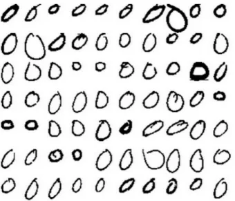
The experiment was done on Concordia University CENPARMI handwritten numeral database. The database contains 6000 samples of 10 numeral classes (each class has 600 samples). Some samples of ‘‘0’’ from the CENPARMI database are shown in Fig. 6.
In the first experiment, we choose the first 200 samples of each class for training, the remaining 400 samples for testing. Thus, the total number of training samples is 2000 while the total number of testing samples is 4000. PCA is used to transform the original 121-dimensional Legendre moment features [28] into D-dimensional features, where D varies from 10 to 100 with an interval 10. Based on the PCA-transformed features, NN, NFL, LRC, SRC, CRC, RSC, RRC_L2 and
B-GRR are employed for classification. The parameter K is set to 200. The
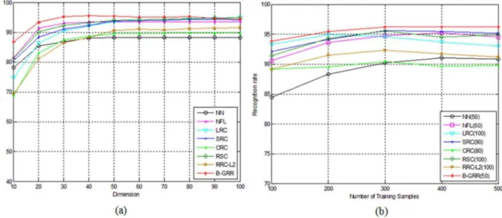
recognition results of each method corresponding to the variation of dimensions is shown in Fig. 7 (a). From Fig. 7 (a), we can see that B-GRR achieves the best results among all competing methods. The maximal recognition rate of B-GRR is 95.4%, compared to 88.3% for NN, 93.6% for NFL, 94.9% for LRC, 89.7% for CRC, 94.3% for SRC, 89.7% for CRC, 95.0% for RSC and 91.5 for RRC_L2. LRC
gives the comparable results since there are enough training samples in each class. In the second experiment, we let the number of training samples per class vary from 100 to 500 with an interval of 100, and the rest samples for testing. Then, PCA is used to transform the original Legendre moment features into low-dimensional features. We select the optimal dimension of each method based on Fig. 6. Some samples in CENPARMI database.
the above experiments as shown in Fig. 7 (b). The recognition rates of each method corresponding to the variation of training samples is shown inFig. 7 (b). From Fig. 7 (b), we can see that B-GRR still gives better results than other competing methods.
NUST603 Database
The experiment was performed on the NUST603 handwritten Chinese character database which was built in Nanjing University of Science and Technology. The database contains 19 groups of Chinese characters that are collected from bank checks, each group with 400 samples. Some images from the NUST603HW database are shown in Fig. 8.
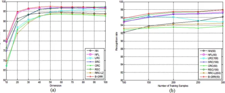
In this experiment, the first 200 samples of each class are used for training, and the remaining samples for testing. Similar to the experimental methodology adopted in the last experiment. PCA is used to transform the original 128-dimensional peripheral feature [29] into D-dimensional features. We thus let D varies from 10 to 100 with interval 10. The parameter K is set to 300. Then NN, NFL, LRC, SRC, CRC, RSC, RRC_L2 and B-GRR are employed for classification.
The performances of each method versus the variation of dimensions are shown in Fig. 9 (a). Additionally, we also let the number of training samples per class vary from 100 to 300 with an interval of 50, and the remaining samples for testing. PCA is then used to transform the original feature into low-dimensional features. We select the optimal dimension of each method based on the above experiments as shown in Fig. 9 (b). The recognition rates of each method are illustrated in Fig. 9 (b). The results inFig. 9are basically consistent with those inFig. 7. B-GRR Fig. 7. (a) The recognition rate of each method for handwritten numeral recognition on the CENPARMI database versus the variation of dimensions; (b) The recognition rate of each method corresponds to the number of classs training samples that varies from 100 to 500 with an inerval 100.The number in brakets of each method means the number of low dimentional trasforamation features.
still achieves the better performance than other methods, irrespective of the variation of dimensions or training sample sizes.
B. Face Recognition without Occlusion
We evaluate the performance of R-GRR on the AR and the Extended Yale B database with illumination and expression changes but without occlusion. In these experiments, PCA is first used to reduce the dimensionality of face image. Fig. 8. Some samples in NUST603HW database.
doi:10.1371/journal.pone.0115214.g008
Fig. 9. (a) The recognition rate of each method for handwritten numeral recognition on the NUST603 database versus the variation of dimensions; (b) The recognition rate of each method corresponds to the number of classs training samples that varies from 100 to 300 with an inerval 50.The number in brakets of each method means the number of low dimentional trasforamation features.
AR Database
The AR face database [26] contains over 4000 color face images of 126 persons, including frontal views of faces with different facial expression, lighting conditions and occlusions. The pictures of 120 individuals were taken in two sessions (separated by two weeks) and each session contains 13 color images. Fourteen face images (each session contains 7) of 100 individuals are selected and used in our experiment. The face portion of each image is manually cropped and then normalized to 60643 pixels.
In this experiment, images from the first session are used for training, and images from the second session are used for testing. Then NFL, LRC, SRC, CRC, B-GRR, RSC, RRC_L2 and the proposed R-GRR are employed for classification.
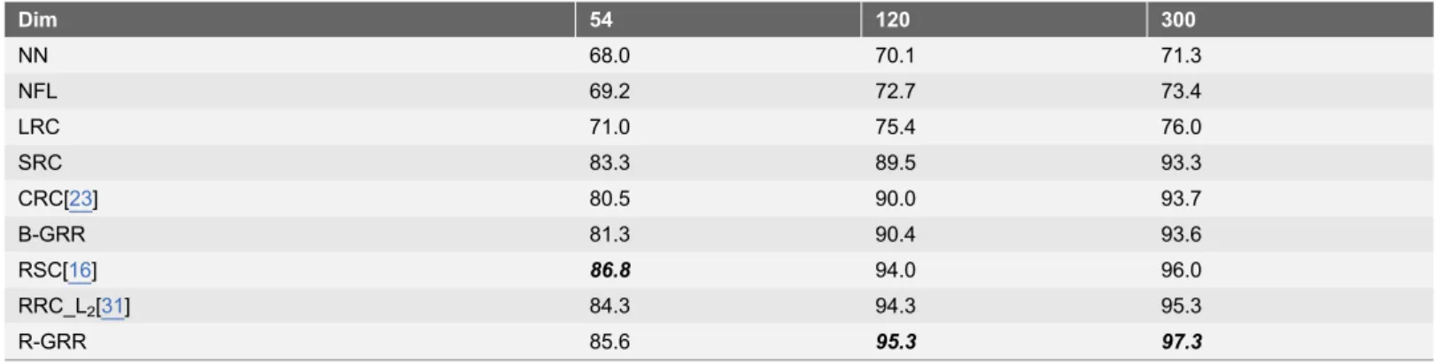
The NN classifier is also used to provide a baseline. The parameter K of R-GRR means we choose the K nearest neighbors of the test image from training set to form the coding dictionary. K is set to 650 here. The recognition rates of each classifier versus the variation of dimensions are listed in Table 1. From Table 1, we can see that our model R-GRR outperforms state-of-the-art methods in all dimensions except that R-GRR is slightly worse than RSC when dimension is 54. However, it’s difficult to achieve better performance when dimension is low for all the methods. The maximal recognition rates of NN, NFL, LRC, SRC, CRC, B-GRR, RSC, RRC_L2 and R-GRR are achieved when the dimension is 300.
Extended Yale B Database
The extended Yale B face image database [27] contains 38 human subjects under 9 poses and 64 illumination conditions. The 64 images of a subject in a particular pose are acquired at camera frame rate of 30 frames/second, so there are only small changes in head pose and facial expression for those 64 images. All frontal-face images marked with P00 are used in our experiment, and each is resized to 48642 pixels.
In our experiment, we use the first 32 images of each individual for training and the remaining images are used for testing. Based on the PCA-transformed features, NN, NFL, LRC, SRC, CRC, B-GRR, RSC, RRC_L2 and R-GRR are employed for classification. The parameter K is 800. The recognition rates of each classifier corresponding to the variation of feature dimensions are listed in Table 2.Table 2 shows that the proposed model R-GRR achieves the best recognition results in all dimensions for face recognition. When the feature dimension is 100, R-GRR gives about 3% improvement of recognition rate over LRC, SRC and CRC, respectively.
C. Face Recognition with Occlusion
In this section, we examine the robustness of R-GRR when face images suffer different occlusions, such as real disguise, block occlusion or pixel corruption. In the following experiments, we mainly compare our method with CRC, SRC, RSC, RRC_L2, correntropy-based sparse representation (CESR) [17] and Gabor-SRC
Face Recognition with Real Disguise
A subset of the AR face image database is used in our experiment. The subset includes 100 individuals, 50 males and 50 females. All the individuals have two session images and each session contains 13 images. The face portion of each image is manually cropped and then normalized to 42630 pixels.
In the first experiment, we choose the first four images (with various facial expressions) from the session 1 and session 2 of each individual to form the training set. The total training images is 800. There are two image sets (with sunglasses and scarves) for testing. Each set contains 200 images (one image per session of each individual with neutral expression). The parameter K is 300 for the test set with sunglasses and 760 for the test set with scarves. The face recognition results of each method on the two testing set are listed inTable 3. FromTable 3, we can see that R-GRR achieves the best recognition results among all the methods when the images with scarves and gives comparable result with the excellent method when the images with sunglasses. Additionally, the performances Table 1.The recognition rate of each classifier for face recognition on the AR database.
Dim 54 120 300
NN 68.0 70.1 71.3
NFL 69.2 72.7 73.4
LRC 71.0 75.4 76.0
SRC 83.3 89.5 93.3
CRC[23] 80.5 90.0 93.7
B-GRR 81.3 90.4 93.6
RSC[16] 86.8 94.0 96.0
RRC_L2[31] 84.3 94.3 95.3
R-GRR 85.6 95.3 97.3
doi:10.1371/journal.pone.0115214.t001
Table 2.The recognition rate of each classifier for face recognition on the Extended Yale B database.
Dim 50 100 200
NN 78.5 85.8 90.2
NFL 88.7 90.5 91.0
LRC 93.3 94.8 95.2
SRC 93.7 94.7 95.6
CRC 91.9 94.7 96.5
B-GRR 92.1 94.9 97.1
RSC 94.2 97.0 98.2
RRC_L2 93.4 97.0 98.3
R-GRR 94.3 97.6 98.4
of RRC_L2, RSC and CESR are higher when facial image with sunglasses.
However, CESR only achieves 42% when facial images with scarves.
In the second experiment, four neutral images with different illumination from the first session of each individual are used for training. The disguise images with various illumination and glasses or scarves per individual in session 1 and session 2 for testing. We set the parameter K as 220, 300, 240 and 320 for the four Table 3.The recognition rate of each classifier for face recognition on AR database with disguise occlusion.
Methods Sunglasses Scarves
CRC 65.5 88.5
SRC 87.0 59.5
GSRC[13] 93.0 79.0
CESR[17] 99.0 42.0
RSC[16] 99.0 97.0
RRC_L2[31] 99.5 96.5
R-GRR 99.5 99.0
doi:10.1371/journal.pone.0115214.t003
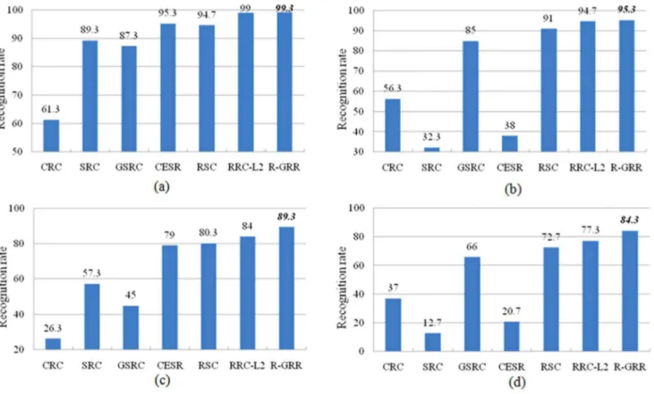
Fig. 10. The recognition rates of each classifier for face recognition on AR database with disguise occlusion.(a) The testing images with sunglasses from session 1; (b) The testing images with scarves from session 1; (c) The testing images with sunglasses from session 2; (d) The testing images with scarves from session 2.
different test sets, respectively. The recognition rates of each method are shown in Fig. 10. From Fig. 10, we can see clearly that R-GRR gives better performance than CRC, SRC, GSRC, CESR, RSC and RRC_L2on different testing subsets. Both
SRC and CESR do well on the subsets with sunglasses but poor in the cases with scarves. However, GSRC achieves better result on the subsets with scarves and worse result on the subsets with sunglasses. Compared to RSC, at least 4.3% improvement is achieved by R-GRR for different testing set. Meanwhile, it is worth noticing that the recognition rate of R-GRR is 67.6%, 59.6% higher than SRC and CESR on the testing images with scarves from session 2, and 43.7% higher than GSRC on the testing images with sunglasses from session 2. In the first two subsets from session 1, the performances of R-GRR and RRC_L2are similar.
However, R-GRR significantly outperforms RRC_L2in the last two subsets (more
challenge tasks) from session 2. Compared with RRC_L2, R-GRR usesk kx 2Q
instead of k kx 22 to refine the regularization term can further improve the classification performance.
Face Recognition with Block Occlusion
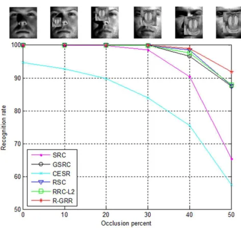
In this experiment, we use the same experiment setting as in [12,16] to test the robustness of R-GRR. Subsets 1 and 2 of the Extended Yale B database are used for training and Subset 3 is used for testing. The face images are resized to 96684.
The parameter K is 500. Fig. 11 shows recognition rates curve of SRC, GSRC, CESR, RSC, RRC_L2 and R-GRR versus the various levels of occlusion (from 0
percent to 50 percent). FromFig. 11, we can see that the proposed R-GRR overall outperforms SRC, GSRC, CESR, RSC and RRC_L2. When the occlusion
percentage is 50%, R-GRR achieves the best recognition rate 91.9, compared to 65.3 for SRC, 87.4 for GSRC, 57.4 for CESR, 87.6 for RSC, and 87.8 for RRC_L2.
It’s surprising that the performance of CESR is very poor. Probably, it is not suitable for dealing with this block occlusion case.
Face Recognition with Pixel Corruption
In this experiment, we chose the images from the Subsets 1 and 2 of the Extended Yale B database for training, and images from the Subset 3 with random pixel corruption (the image is corrupted by using uniformly distributed random values within [0, 255]) for testing. The face images were resized to 96684 pixels. The
corrupted pixels are randomly chosen for each test image and the locations are unknown to the algorithm. We vary the percentage of corrupted pixels from 0% to 90%. Since the most competing methods can achieve better performance from 0% to 40%. We only report the recognition rates for 50%–90% corruption. Fig. 12 plots the recognition rates of five methods under different levels of corruptions. From Fig. 12, we can see that R-GRR, RRC-L2, and RSC give the
D. Discussion
In this section, we first discuss the influences of the parameters K,l1andl2in our experiments. We then compare the running time of the proposed R-GRR with state-of-the-art methods.
The performances of the proposed method R-GRR (or B-GRR) with different parameters are evaluated on different recognition scenarios. The experiments setting are same with the above mentioned experiments in section 5.2 and 5.3. In our experiments, we just change one parameter when fixing the other ones. Fig. 13plots the recognition rates versus the variation of the parameter K on the CENPARMI database and NUST603 database. From Fig. 13, we can see that B-GRR can achieve the better recognition rates in conjunction with a smaller K. Fig. 14 plots the recognition rates versus the variation of the parameter K in different face recognition experiments. From Fig. 14 (a) and (b), we can see that the parameter K is relatively larger and smaller than total number of training samples will lead to higher performance when face images without occlusion. Fig. 14 (c) and (e) show that the recognition rates are not sensitive to the variations of the parameter K. In Fig. 14 (f), the proposed method achieves best results when the K is 200 for the test images with block occlusion. However, R-GRR gives the best performance when the K is set to 550 for the test images with Fig. 11. The recognition rates of SRC, GSRC, CESR, RSC, RRC_L2and R-GRR under the occlusion
percentage from 0 to 50.
pixel corruption as shown in Fig. 14 (g). Generally speaking, the parameter K is relatively smaller in the case that the feature dimension is much lower than the number of training samples, while the parameter K is relatively larger in the case that the feature dimension is much higher than the number of training samples. In this paper, we employ the cross-validation strategy to determine the parameter Fig. 12. The recognition rates of SRC, GSRC, CESR, RSC, RRC_L2and R-GRR under the pixel corruption percentage from 50% to 90%.
doi:10.1371/journal.pone.0115214.g012
Fig. 13. The recognition rate curves of B-GRR versus the variation of parameter K in handwritten numeral recognition tasks.(a) Experiment on the CENPARMI database; (b) Experiment on the NUST603 database.
K in the training stage. Specifically, we select one training sample as query sample and the rest training samples as gallery set. Thus, the recognition rate of all training samples can be achieved. We choose the best parameter K which achieves the best recognition rate.
Fig. 15plots the recognition rates versus the variation of the regularization parameters l1 andl2, respectively. FromFig. 15, we can see that the proposed model always achieves it optimal or nearly optimal performance when l2~1 under different face recognition scenarios. However, the performance of the proposed model is non-sensitive to the variation of l1. Thus, it’s easy to set the regularization parameters of the proposed methods in real-world applications.
The running time of the competing methods, including SRC, GSRC, CESR, RSC, RRC_L2 and R-GRR, are evaluated on the AR database (with sunglasses).
The programming environment is Matlab version 11b. The desktop used is of 2.93 GHz CPU and with 4G RAM. Table 4lists the computation time for one recognition operation of various methods with the same experiment setting in Fig. 14. The recognition rate curves of R-GRR versus the variation of parameter K on the different experiments.(a) the images without occlusion for test; (b) the images without occlusion for test; (c) the images with sunglasses for test; (d) the images with scarf for test; (e) the images with sunglasses (sg-X) or scarf (sc-X) in session X for test; (f) the images with block occlusion (50%) for test; (g) the images with pixel corruption (90%) for test.
Section 5.3.1. Note that we only compute the online running time for R-GRR. From Table 4, we can see that R-GRR is superior to SRC, GSRC and RSC due to less computation cost and better performance. RRC_L2 achieves the least
computation time. SRC has rather high computation burden. In addition, RSC is very time-consuming since it must solve L1 optimization problem in each
iteration process. Although CESR is also fast, its performance is not stable. R-GRR gives comparable computation time with RRC_L2 and achieves better
perfor-mance than RRC_L2 in most cases.
Conclusions and Future Works
In this section, we first conclude the paper and then give more discussions on potential future work.
Fig. 15. The recognition rate curves of the proposed model versus the variation of regularization parameters on the different experiments.(a) The influence ofl1. (b) The influence ofl2.
doi:10.1371/journal.pone.0115214.g015
Table 4.Computation time of R-GRR and state-of-the-art methods.
Methods Time (s)
SRC 96.5
GSRC 12.3
CESR 0.36
RSC 142.9
RRC_L2 0.21
R-GRR 0.24
This paper presents a general regression and representation (GRR) model for pattern classification. In GRR, we learn the prior information from the training set by using the generalized Tikhonov regularization and KNN, and obtain the specific information from the test sample by using the iteratively reweighted algorithm. Actually, we provide two classifiers: B-GRR and R-GRR, which combine the prior information and the specific information with different strategies. Experimentson character datasets and face datasets demonstrate that the validity of our model and its performance advantages over state-of-the-art classification methods. Particularly, R-GRR achieves encouraging recognition rates under different cases but with lower computational cost.
Although our model has demonstrated promising performance, there are still many issues requiring in-depth investigation in the future. Here, two improve-ments can be made for GRR. (1) Most classification methods perform well on the condition that they assume the training and testing data are drawn from the same feature space and the same distribution. However, it’s difficult to hold this assumption in real-world applications. To address this problem, transfer learning is proposed and aims to help improve the target predictive function using the knowledge in source domain [50]. Deng et al. presented the generalized hidden-mapping ridge regression method for various types of classical intelligent methods [51]. We can borrow the idea of transfer learning to improve the robustness of our model. (2) With the ever increasing size of training data sets, a challenge in our model is how to design an efficient learning algorithm. Actually, there are many literatures have been reported to overcome the similar problem. IvorW. Tsang et al. presented a core vector machine (CVM) to handle larger datasets.
Furthermore, CVM not only preserves the performance of SVM but also performs much faster than existing scale-up methods [52]. Deng et al also developed effective learning algorithms for fussy models when facing with large datasets [53,54].
Ethics Statement
Some face image datasets were used in this paper to verify the performance of our methods. These face image datasets are publicly available for face recognition research, and the consent was not needed. The face images and the experimental results are reported in this paper without any commercial purpose.
Author Contributions
Conceived and designed the experiments: JJQ JY. Performed the experiments: JJQ. Analyzed the data: JJQ JY YX. Wrote the paper: JJQ JY YX.
References
2. Chien JT, Wu CC(2002) Discriminant waveletfaces and nearest feature classifiers for face recognition, IEEE TPAMI, vol. 24, no. 12, pp. 1644–1649.
3. Laaksonen J(1997) Local subspace classifier. In Proc. Int. Conf. Artif. Neural Netw, pp. 637–642.23
4. Li SZ(1998) Face recognition based on nearest linear combinations, In CVPR, pp. 839–844.
5. Vinje W, Gallant J(2000) Sparse Coding and Decorrelation in Primary Visual Cortex During Natural Vision, Science, Vol. 287. no. 5456, pp. 1273–1276
6. Olshausen BA, Field DJ(2004) Sparse coding of sensory inputs, Current Opinion in Neurobiology, Vol. 14, No. 4, pp. 481–487.
7. Serre T(2006) Learning a Dictionary of Shape-Components in Visual Cortex: Comparison with Neurons, Humans and Machines, PhD dissertation, MIT.
8. Zhou H, Hastie T, Tibshirani R (2004) Sparse principle component analysis. Technical Report, Statistics Department, Stanford University.
9. Yang JC, Wright J, Huang T, Ma Y(2008) Image Super-resolution as Sparse Representation of Raw Image Patches, InCVPR.
10. Mairal J, Sapiro G, Elad M(2008) Learning multiscale sparse representations for image and video restoration,SIAM MMS7(1): 214–241.
11. Yang J, Yu K, Gong Y, Huang T(2009) Linear spatial pyramid matching using sparse coding for image classification, InCVPR.
12. Wright J, Yang A, Ganesh A, Sastry SS, Ma Y (2009) Robust face recognition via sparse representation.IEEE T PAMI31(2): 210–227.
13. Yang M, Zhang L(2010) Gabor Feature based Sparse Representation for Face Recognition with Gabor Occlusion Dictionary. InECCV.
14. Yang J, Zhang L, Xu Y, Yang JY (2012) Beyond Sparsity: the Role of L1-optimizer in Pattern Classification, Pattern Recognition 45: 1104–1118
15. Wright J, Ma Y, Mairal J, Sapiro G, Huang T, et al.(2010) Sparse representation for computer vision and pattern recognition. Proceedings of IEEE, Special Issue on Applications of Compressive Sensing & Sparse Representation 98(6): 1031–1044.
16. Yang M, Zhang L, Yang J, Zhang D(2011) Robust sparse coding for face recognition, InCVPR.
17. He R, Zheng WS, Hu BG (2011) Maximum correntropy criterion for robust face recognition, IEEE T PAMI., vol. 33, no. 8, pp. 1561–1576.
18. He R, Zheng WS, Hu BG, Kong XW(2011) A regularized correntropy framework for robust pattern recognition, Neural Computation vol. 23, pp. 2074–2100.
19. Naseem I, Togneri R, Bennamoun M (2010) Linear regression for face recognition. IEEE T PAMI 32(11): 2106–2112.
20. Xu Y, Zhu Q, Fan Z, Zhang David, Mi J, et al.(2013) Using the idea of the sparse representation to perform coarse-to-fine face recognition, Information Sciences 238: 138–148
21. Rigamonti R, Brown M, Lepetit V (2011) Are Sparse Representations Really Relevant for Image Classification? InCVPR.
22. Shi Q, Eriksson A, Hengel A, Shen C(2011) Is face recognition really a compressive sensing problem? InCVPR.
23. Zhang L, Yang M, Feng XC(2011) Sparse representation or collaborative representation which helps face recognition? InICCV.
24. Yang M, Zhang L, Zhang D, Wang SL (2012) Relaxed Collaborative Representation for Pattern Classification, InCVPR.
25. Kim SJ, Koh K, Lustig M, Boyd S, Gorinevsky D(2007) A interiorpoint method for largescale l1 -regularized least squares.IEEE Journal on Selected Topics in Signal Processing1(4): 606–617.
26. Martinez A, Benavente R(1998) The AR face database. Technical Report 24, CVC.
28. Liao SX, Pawlak M(1996) On image analysis by moments, IEEE T PAMI 18(3): 254–266.
29. Tseng YH, Kuo CC, Lee HJ (1998) Speeding Up Chinese Character Recognition in An Automatic Document Reading System, Pattern Recognition 31(11): 1601–1612.
30. Wikipedia.Available:http://en.wikipedia.org/wiki/Ridge_regression. Accessed 2014 Nov 27.
31. Yang M, Zhang L, Yang J, Zhang D(2013) Regularized Robust Coding for Face Recognition.IEEE Trans. on Image Processing22(5): 1753–1766.
32. Yang M, Zhang L, Simon CK, Zhang D (2013) Gabor feature based robust representation and classification for face recognition with Gabor occlusion dictionary, Pattern Recognition 46: 1865–1878.
33. Xu Y, Zhu X, Li Z, Liu G, Lu Y, et al.(2013) Using the original and ‘symmetrical face’ training samples to perform representation based two-step face recognition, Pattern Recognition 46: 1151–1158.
34. Zhang B, Karray F, Li Q, Zhang L(2012) Sparse Representation Classifier for microaneurysm detection and retinal blood vessel extraction, Information Sciences 200: 78–90.
35. He R, Hu B, Zheng W, Guo Y(2010) Two-stage Sparse Representation for Robust Recognition on Large-scale Database. In Twenty-Fourth AAAI Conference on Artificial Intelligence (AAAI).
36. Qian J, Yang J(2013) General Regression and Representation Model for Face Recognition, Biometrics workshop in conjunction with CVPR.
37. Theodorakopoulos I, Rigas I, Economou G, Fotopoulos S(2011) Face recognition via local sparse coding, InICCV1647–1652.
38. He R, Zheng WS, Tan T, Sun Z(2014) Half-quadratic based iterative minimization for robust sparse representation. IEEE Trans. on Pattern Analysis and Machine Intelligence (TPAMI) 36(2): 261–275.
39. Gao S, Tsang Ivor WH, Chia LT(2013) Sparse Representation with Kernels,IEEE Trans. on Image Processing22 (2): 423–434.
40. Zhou Z, Wagner A, Mobahi H, Wright J, Ma Y(2009) Face Recognition With Contiguous Occlusion Using Markov Random Fields. InICCV.
41. Li XX, Dai DQ, Zhang XF, Ren CX(2013) Structured Sparse Error Coding for Face Recognition With Occlusion,IEEE Trans.on Image Processing 22(5): 1889–1999.
42. Ou W, You X, Tao D, Zhang P, Tang Y, et al.(2014) Robust face recognition via occlusion dictionary learning,Pattern Recognition47(4): 1559–1572.
43. Theodorakopoulos, Economou, Fotopoulos (2013) Collaborative Sparse Representation in Dissimilarity Space for Classification of Visual Information,ISVC, LNCS 8033: 496–506.
44. Tikhonov AN, Goncharsky AV, Stepanov VV, Yagola AG(1995) Numerical Methods for the Solution of Ill-Posed Problems, Kluwer Academic Publishers.
45. Roy DM, Delphine JR, Massart De´sire´ L (2000) The Mahalanobis distance, Chemometrics and Intelligent Laboratory Systems, 50: 1–18.
46. Kuan CM(2004) Statistics: Concepts and Methods, 2nd edition (in Chinese), Taipei: Hua-Tai Publisher.
47. Kariya T, Kurata H(2004) Generalized least squares. John Wiley & Sons.
48. He R, Tan T, Wang L, Zheng W(2012) L21 Regularized Correntropy for Robust Feature Selection. In CVPR.
49. Zhang Y, Sun Z, He R, Tan T(2013) Robust Subspace Clustering via Half-Quadratic Minimization, In ICCV.
50. Pan J, Yang Q (2010) A survey on transfer learning. IEEE Transactions on Knowledge and Data Engineering 22.10: 1345–1359.
51. Deng Z, Choi K, Jiang Y, Wang S(2014) Generalized Hidden-Mapping Ridge Regression, Knowledge-Leveraged Inductive Transfer Learning for Neural Networks, Fuzzy Systems and Kernel Methods, IEEE Transactions on Cybernetics, DOI: 10.1109/TCYB.2014.2311014.
53. Deng Z, Choi K, Cao L, Wang S(2014) T2FELA: Type-2 Fuzzy Extreme Learning Algorithm for Fast Training of Interval Type-2 TSK Fuzzy Logic System. IEEE Trans. Neural Netw. Learning Syst 25(4): 664–676.