Solution of second order linear fuzzy difference equation by
Lagrange’s multiplier method
Sankar Prasad Mondal1*, Dileep Kumar Vishwakarma1, Apu Kumar Saha1
(1) Department of Mathematics, National Institute of Technology, Agartala, Jirania-799046, Tripura, India.
Copyright 2016 © Sankar Prasad Mondal, Dileep Kumar Vishwakarma and Apu Kumar Saha. This is an open access article distributed under the Creative Commons Attribution License, which permits unrestricted use, distribution, and reproduction in any medium, provided the original work is properly cited.
Abstract
In this paper we execute the solution procedure for second order linear fuzzy difference equation by Lagrange’s multiplier method. In crisp sense the difference equation are easy to solve, but when we take in fuzzy sense it forms a system of difference equation which is not so easy to solve. By the help of Lagrange’s multiplier we can solved it easily. The results are illustrated by two different numerical examples and followed by two applications.
Keywords: Fuzzy number, Second order fuzzy difference equation, Lagrange’s multiplier.
1 Introduction
1.1. Fuzzy sets, fuzzy number and generalized fuzzy number
In 1965, Lotfi A. Zadeh [1], a professor of electrical engineering at the University of California in Berkeley, published the papers on his new theory of Fuzzy Sets and Systems. After then various researcher contribute in that topic. Since the 1980s, this mathematical theory of the concept “un-sharp amounts” has been applied with great success in many different fields of research. Since Chang and Zadeh [2] introduced the concept of fuzzy numbers in 1972. A lot of mathematicians have been studying them (one-dimension or n-dimension fuzzy numbers, see for example [3,4,5,6]) and try to modeled with it. With the development of theories and applications of fuzzy numbers, this concept becomes more important for modeling.
Most of the researcher take a fuzzy number with maximum gradation one. Now it is not necessary that the maximum gradation is one. Ii is difference for one to one. So we can make it generalized. That is the gradation is greater than zero and less than or equal to one. Many researchers use the concepts of generalized fuzzy number for their research such as [7,8,9,10].
1.2. Necessity for difference equation and fuzzy difference
In modeling of real natural phenomena, difference equations also play an important role in many areas of discipline, exemplary in economics, biomathematics, science and engineering. Many experts in such areas
Available online at www.ispacs.com/jsca
Volume 2016, Issue 1, Year 2016 Article ID jsca-00063, 17 Pages
doi:10.5899/2016/jsca-00063
widely use difference equations in order to make some problems under study more comprehensible. In many cases, information about the physical phenomena related is always immanent with uncertainty.
1.3. Difference equation
Recently the study of the qualitative behavior of difference equation and difference equation system is a which topic of a great interest. A difference equation is an equation specifying the change in a variable between two periods. By using the difference equation we can study the concerning factors, which cause the change in the value of the given functions in different time periods. it is known that difference equation appears naturally as discrete analogous having many applications in computer science, control engineering, ecology, population dynamics, queuing problems, statistical problems, stochastic time sires, geometry, psychology, sociology physics economics engineering etc. The theory of difference equations developed greatly during last three decay. The theory of difference equation occupies a important position in different fields. No doubt the theory of difference equation in play important role in mathematics as well as its applications. More over the data are absorbed in relation with a real world phenomenon that can be described by difference equations.
1.4. Fuzzy difference equation
A difference fuzzy equation is a fuzzy difference equation when (i) initial condition is fuzzy number, (ii) coefficients is fuzzy number, (iii) initial conditions and coefficients are both fuzzy numbers. Fuzzy difference equation growing rapidly developed for the many years. Now the problem is that the solution procedure of difference equation and fuzzy difference are not same. To study the behavior and solutions of a fuzzy difference equation we need to study the concepts of fuzzy difference, since the fuzzy difference is not same as crisp difference. We can show that every fuzzy difference can converted to system of fuzzy difference equations.
1.5. Review on fuzzy difference equation
There exist several research papers where difference equation is solved with fuzzy environment. Now we concentrate some published paper:
In [11] Deeba et.al. solve a fuzzy difference equation with an applications. The model of CO2 level in blood is modeled with fuzzy difference equation and solved by Deeba et.al by [12]. Lakshmikantham and Vatsala [13] discuss the basic theory of fuzzy difference equations. Papaschinopoulos et.al. [14,15]. Papaschinopoulos and Schinas [16] discuss the behavior and solution of some different type of fuzzy difference equations. Papaschinopoulos and Stefanidou [17] give a description on boundedness and asymptotic behavior of the solutions of a fuzzy difference equation. Umekkan et.al. [18] give a application of finance in fuzzy difference equation. Stefanidou et.al. [19] give brief discussion on an exponential type fuzzy difference equation. The asymptotic behavior of a second order fuzzy difference equation is delivered by Din [20]. The behavior of solutions to a fuzzy non linear difference equation are treated by Zhang et.al. [21]. Memarbashi and Ghasemabadi [22] solved fuzzy defference equation of volterra type. A fuzzy difference equation of rational form were solved by Stefanidou and Papaschinopoulos [23]. The application of fuzzy difference equation in finance is consider by Konstantinos et.al. [24].
1.6. Motivation
1.7.Novelties
In spite the above mention developments few developments can still be done by our self which are:
(i) Difference equation is defined in fuzzy environment i.e., only initial conditions are fuzzy number, only coefficients are fuzzy number and both initial condition and coefficients are fuzzy number.
(ii) Difference equation is solved with fuzzy initial condition i.e, initial condition is fuzzy number. (iii) The solutions are found by Lagrange’s multiplier method.
(iv) Proposed method is illustrated by two numerical example and two applications.
1.8. Structure of the paper
The structure of the paper is as follows: In first section we introduce the previous work on fuzzy set theory and fuzzy difference equation. Second section goes to preliminary concept. We define difference equation in third section. In fourth section we define fuzzy difference equation. In fifth section we solve second order fuzzy difference equation with initial value as fuzzy number by Lagrange’s multiplier method. In sixth section the numerical examples are illustrated. The applications are given in seventh section. The conclusion is done in eighth section.
2 Preliminaries
Definition 2.1
Fuzzy Set: A fuzzy set �̃ is defined by �̃ = {( , �̃ ): ∈ �, �̃ ∈ [ , ]}. In the pair ( , �̃ ) the first element belong to the classical set �, the second element �̃ , belong to the interval [ , ], called Membership function.
Definition 2.2
�-cut of a fuzzy set: The �-level set (or interval of confidence at level � or �-cut) of the fuzzy set �̃ of X is a crisp set �� that contains all the elements of X that have membership values in �̃ greater than or equal to
� i.e. �̃ = { : �̃ �, ∈ �, � ∈ [ , ]}.
Definition 2.3
Fuzzy Number:[25] A fuzzy number is fuzzy set like : � → � = [ , ] which satisfies (1) is upper semi-continuous.
(2) = outside the interval [ , ]
(3) There are real numbers , such and
(3.1) is monotonic increasing on [ , ], (3.2) is monotonic decreasing on [ , ],
(3.3) = ,
Let be the set of all real fuzzy numbers which are normal, upper semi-continuous, convex and compactly supported fuzzy sets.
Definition 2.4
Fuzzy Number (Parametric form): [26] A fuzzy number in a parametric form is a pair , of
function , , , which satisfies the following requirments:
(1) is a bounded monotonic increasing left continuous function, (2) is a bounded monotonic decreasing left continuous function,
(3) , .
definitions, the fuzzy number space {( , )} becomes a convex cone which could be embedded isomorphically and isometrically into a Banach space [27, 28].
Definition 2.5
[29] Let = , , = , ∈ , and arbitrary � ∈ �.
Then
(1) = iff = and = ,
(2) + = + , + ,
(3) − = ( − , − ),
(4) � = {(�� , �, � ), � <, �
Definition 2.6
[30]For arbitrary = , , = , ∈ , the quantity
, = ∫ − + ∫ −
Is the distance between fuzzy numbers and .
Definition 2.7
Triangular Fuzzy Number: A Triangular fuzzy number (TFN) denoted by �̃ is defined as , , where the membership function
�̃ =
{
, −
− , , =
− − , ,
Definition2.8
�-cut of a fuzzy set �̃: The �-cut of �̃ = , , is given by
�� = [ + � − , − � − ], ∀ � ∈ [ , ]
Theorem 2.1
Let � be an interval of real numbers, and let �: � × � → �be a continuous function. Consider the difference equation
x + = f x , x − , n = , , …, (2.1)
Where the initial values − , ∈ �. and � satisfies the following conditions:
(1) There exist positive number and with < such that � , for all , ∈ [ , ].
(2) � , is increasing in ∈ [ , ] for each ∈ [ , ], and � , is decreasing in ∈ [ , ] for each
∈ [ , ].
Then there exists exactly one equilibrium solution x̅ (1) which lies in [a, b]. Moreover, every solution of (2.1) with initial conditions x− , x ∈ [a, b] converges to x̅.
3 Difference equation
A - th order linear difference equation (synonymously, a linear recurrence relation) is a set of equations of the form
�− ( �− �− + �− �− + ⋯ … … … + �−� �−�) = � (3.2)
For = , + , … … …
If �= , for all , the equation is said to be a homogeneous difference equation otherwise it is non homogeneous difference equation. The term � is called the forcing factor.
Now if � (� = , , … . , ) do not depend on then the equation said to have constant, coefficients.
4 Fuzzy difference equation
Consider the second order non homogeneous difference equation as
�+ + �+ + �= � (4.3)
With initial condition �= = and �= =
The above second order difference equation is called fuzzy difference equation if any of one case is followed by the above difference equation:
(1) The initial condition or conditions are fuzzy number (Type I) (2) The coefficient or coefficients are fuzzy number (Type II)
(3) The initial condition or conditions and coefficient or coefficients are fuzzy numbers (Type III)
5 Exact solution of second order difference equation with fuzzy initial value
5.1. Formulation of second order difference equation with fuzzy initial value
Consider the second order non homogeneous difference equation as
�+ + �+ + �= � (5.4)
With initial condition ̃�= = ̃ and ̃�= = ̃
Different cases can be arising. If we take different sign of , and then the different cases are as follows:
(i) > , > , >
(ii) > , < , > (iii) > , > , < (iv) > , < , <
(v) < , > , >
(vi) < , < , > (vii) < , > , < (viii) < , < , <
Note: In crisp sense the above all cases are equal. But in fuzzy sense they are not same.
For proving these we take the cases (iv) and (viii).
Case (iv): For case (iv) if we take the �-cut the we get
[ �+ , � , �+ , � ] + [ �+ , � , �+ , � ] + [ �, � , �, � ] = [� , � ]
{ �+ , � + �+ , � + �, � = �
�+ , � + �+ , � + �, � = � (5.5)
Case (viii):
For case (viii) if we take the �-cut the we get
[ �+ , � , �+ , � ] + [ �+ , � , �+ , � ] + [ �, � , �, � ] = [� , � ]
i.e.,
{ �+ , � + �+ , � + �, � = �
�+ , � + �+ , � + �, � = � (5.6)
Clearly (5.5) and (5.6) are not same.
5.2. Exact solution of second order difference equation with fuzzy initial value by Lagranges multiplier method
There can be various cases. For simplicity of the paper we take only one case Now consider a simple case: > and , <
Now taking the �-cut of the above equation we get
[ �+ , � , �+ , � ] + [ �+ , � , �+ , � ] + [ �, � , �, � ] = [� , � ]
Or,
�+ , � + �+ , � + �, � = � (5.7)
and
�+ , � + �+ , � + �, � = � (5.8)
With initial value
, � = �
, � = �
, � = �
, � = �
The above equations are system of difference equation
Multiplying the equation (5.8) by and adding with (5.7) we get
[ �+ , � + �+ , � ] + [ �+ , � + �+ , � ] + [ �, � + �, � ] = [� +
� ]
Or, [ �+ , � + �+ , � ] +�
� [ �+ , � +� �+ , � ] +
�
� [ �, � +� �, � ] = [ +
]� (5.9)
Take =
� i.e., = ±
When = the above equation becomes
[ �+ , � + �+ , � ] + [ �+ , � + �+ , � ] + [ �, � + �, � ] = � (5.10)
Or,
�+ � + �+ � + � � = �
Where, � � = �, � + �, �
When = − the above equation becomes
[ �+ , � − �+ , � ] − [ �+ , � − �+ , � ] − [ �, � − �, � ] = �
�+ � + �+ � + � � = (5.11)
Where, � � = �, � − �, �
Clearly it is easy to solve (5.10) and (5.11).
After solving the difference equation we can find � � and � � . Then we can write
�, � = �� + � � and �, � = � � − ��
The others cases can be done in similar way.
6 Numerical example
Example 6.1
Let the difference equation is �+ − �+ + � = with fuzzy initial condition = , , and =
, , . Then find �.
Solution: Taking � cut of the difference equation
( �+ , � , �+ , � ) − ( �+ , � , �+ , � ) + ( �, � , �, � ) = , (6.12)
i.e.,
�+ , � − �+ , � + �, � = (6.13) �+ , � − �+ , � + �, � = (6.14)
Multiplying by in equation (6.14) and adding with equation (6.13) we have
( �+ , � − �+ , � + �, � ) + ( �+ , � − �+ , � + �, � ) =
Or,
( �+ , � + �+ , � ) − � �+ , � + �+ , � + ( �, � + �, � ) = (6.15)
Taking =
� or, = ±
If = the above equation implies
( �+ , � + �+ , � ) − ( �+ , � + �+ , � ) + ( �, � + �, � ) = (6.16)
Let �, � + �, � = � �
Then obviously �+ , � + �+ , � = �+ � and �+ , � + �+ , � = �+ � Therefore the equation (6.16) becomes
�+ � − �+ � + � � = (6.17)
Put = − in equation (6.15)
( �+ , � − �+ , � ) + (− �+ , � + �+ , � ) + ( �, � − �, � ) = (6.18)
Let �, � − �, � = � �
Then obviously �+ , � − �+ , � = �+ � and �+ , � − �+ , � = �+ � Therefore the equation (6.18) becomes
�+ � − �+ � + � � = (6.19)
Solving (6.17) and (6.19) we can find � � and � �
Now we find the value of �, � , �, � from the above relation
{ �, � =
� � + ��
�, � = � � − ��
We have system of fuzzy difference equation (6.17) and (6.19) whose general solution is
� � = � �+ � �
� � = � ��+ � �
Therefore the general solution is
�, � = { � + � } �+ { � + � } �
�, � = { � − � } �+ { � − � } �
Therefore using initial condition we get from (6.17) and (6.19) we get
�, � = � − �+ − � �
and
�, � = + � �+ − � �
Therefore the general solution of the main equation is written as
�, � = (− + �) �+ ( + �) �
�, � = (− − �) �+ ( − �) �
Table 1: Solution for different values of
= =
� �, � �, � � �, � �, �
0 52.0000 80.0000 0 484.0000 728.0000 0.1 53.4000 78.6000 0.1 496.2000 715.8000 0.2 54.8000 77.2000 0.2 508.4000 703.6000 0.3 56.2000 75.8000 0.3 520.6000 691.4000 0.4 57.6000 74.4000 0.4 532.8000 679.2000 0.5 59.0000 73.0000 0.5 545.0000 667.0000 0.6 60.4000 71.6000 0.6 557.2000 654.8000 0.7 61.8000 70.2000 0.7 569.4000 642.6000 0.8 63.2000 68.8000 0.8 581.6000 630.4000 0.9 64.6000 67.4000 0.9 593.8000 618.2000 1 66.0000 66.0000 1 606.0000 606.0000
= =
� �, � �, � � �, � �, �
Figure 1: Figure of �, � and �, � for different values of
Description and discussion on the table: (i), (ii), (iii) and (iv) are the figure for
�, � and �, � for = , , and 8 respectively. Clearly for all fixed , �, � is increasing and �, � is a decreasing function as � goes from 0 to 1. Hence the solution is a strong solution.
Example 6.2
Let the difference equation is �+ − � = with initial condition = , , and = , , . Then find �.
Solution: Taking � cut of the difference equation
( �+ , � , �+ , � ) − ( �, � , �, � ) = , (6.21)
which implies
�+ , � − �, � = (6.22)
and
�+ , � − �, � = (6.23)
Multiplying by in equation (6.23) and adding with (6.22) we get
( �+ , � + �+ , � ) + (− �, � − �, � ) =
Or,
( �+ , � + �+ , � ) + −� �, � − �, � = (6.24)
Taking =
� i.e., = + , −
Now putting = in (6.24) we get
Putting = − in (6.24) we get
( �+ , � − �+ , � ) + � � − � � = (6.26)
Let � � = �, � + �, � and � � = �, � − �, � then (6.25) and (6.26) becomes
�+ � − � � = (6.27) �+ � + � � = (6.28)
The general solution of (6.27) and (6.28) are
� � = � cos��+ � sin�� and � � = � cos��+ � sin��
Therefore the general solution of main equation is written as
�, � = � � + � � = �− [{ � + � } cos �+ { � + � } sin �]
and
�, � = � � − � � = �− [{ � − � } cos �+ { � − � } sin �]
Therefore the solution is
�, � = + � cos �+ + � sin �
and
�, � = − � cos �+ − � sin �
Table 2: Solution for different values of
= =
� �, � �, � � �, � �, �
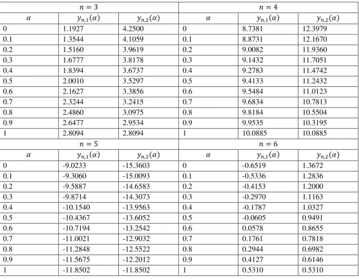
0 1.1927 4.2500 0 8.7381 12.3979
0.1 1.3544 4.1059 0.1 8.8731 12.1670 0.2 1.5160 3.9619 0.2 9.0082 11.9360 0.3 1.6777 3.8178 0.3 9.1432 11.7051 0.4 1.8394 3.6737 0.4 9.2783 11.4742 0.5 2.0010 3.5297 0.5 9.4133 11.2432 0.6 2.1627 3.3856 0.6 9.5484 11.0123 0.7 2.3244 3.2415 0.7 9.6834 10.7813 0.8 2.4860 3.0975 0.8 9.8184 10.5504 0.9 2.6477 2.9534 0.9 9.9535 10.3195
1 2.8094 2.8094 1 10.0885 10.0885
= =
� �, � �, � � �, � �, �
Figure 2: Figure of �, � and �, � for different values of
Description and discussion on the table: (i), (ii), (iii) and (iv) are the figure for
�, � and �, � for = , , and 6 respectively. Clearly for all fixed , �, � is increasing and �, � is a decreasing function as � goes from 0 to 1. Hence the solution is a strong solution.
7 Application
Application 1: In a new colony of geese there are 10 pairs of bird home of which procreate eggs in their first year. In each next year, pair of birds which are in there are in second or latter year have, on average 4 eggs (2 male or female). Assuming no death is in the problem.
The difference equation which describe the geese population is
+ = + −
Where represents the geese population (in pairs at the beginning of the -th year)
Application 2: A pair of hares required a maturation period of one month before they can make off spring. Each pair of mature hares presents at end of one month produce two new pairs by the end of next month. If indicate the number of pairs alive at the end of nth month and no hares die, satisfies the difference
equation = − + −
Solve the both problem (Application 1 and Application 2) with initial condition as. = ̃ = , , and
= ̃ = , , .
+ = + − with initial condition = ̃ , = ̃ (7.29)
Taking � cut of the difference equation is
( + , � , + , � ) = ( , � , , � ) + ( − , � , − , � )
i.e.,
+ , � − , � − − , � = (7.30) + , � − , � − − , � = (7.31)
We have from equation (7.30)
+ , � − , � − − , � =
The auxiliary equation is − − = , whose roots are = − , (Distinct real roots) So, the general solution is
, � = − +
Using initial condition we have
� = +
� = − +
, � = � − � − + � + �
From equation (7.31)
+ , � − , � − − , � =
The auxiliary equation is − − = , whose roots are = − , (Distinct real roots) The general solution is written as
, � = − +
Using initial condition
� = +
� = − + Solving we get
, � = � − � − + � + �
The required solution of fuzzy difference equation is
, � = � − � − + � + �
, � = � − � − + � + �
Numerical: The solutions are
, � = � − + + �
Table 3: Solution for different values of
= =
� , � , � � , � , �
0 64.0000 98.0000 0 256.0000 386.0000 0.1 65.7000 96.3000 0.1 262.5000 379.5000 0.2 67.4000 94.6000 0.2 269.0000 373.0000 0.3 69.1000 92.9000 0.3 275.5000 366.5000 0.4 70.8000 91.2000 0.4 282.0000 360.0000 0.5 72.5000 89.5000 0.5 288.5000 353.5000 0.6 74.2000 87.8000 0.6 295.0000 347.0000 0.7 75.9000 86.1000 0.7 301.5000 340.5000 0.8 77.6000 84.4000 0.8 308.0000 334.0000 0.9 79.3000 82.7000 0.9 314.5000 327.5000 1 81.0000 81.0000 1 321.0000 321.0000
= =
� , � , � � , � , �
Figure 3: Figure of , � and , � for different values of
Description and discussion the figure and table: (i), (ii), (iii) and (iv) are the figure for
, � and , � for = , , and 10 respectively. Clearly for all fixed , , � is increasing and , � is a decreasing function as � goes from 0 to 1. Hence the solution is a strong solution.
8 Conclusion
References
[1] L. A. Zadeh, Fuzzy sets, Information and Control, 8 (1965) 338-353. http://dx.doi.org/10.1016/S0019-9958(65)90241-X
[2] S. S. L. Chang, L. A. Zadeh, On fuzzy mappings and control, IEEE Trans. Syst. Man Cybernet, 2 (1972) 30-34.
http://dx.doi.org/10.1109/TSMC.1972.5408553
[3] P. Diamond, P. Kloeden, Metric Spaces of Fuzzy Sets: Theory and Applications, World Scientific, Singapore, (1994).
[4] D. Dubois, H. Prade, Operations on fuzzy numbers, Internat. J. Systems Sci. 9 (1978) 613-626. http://dx.doi.org/10.1080/00207727808941724
[5] R. Goetschel, W. Voxman, Elementary calculus, Fuzzy Sets and Systems 18 (1986) 31-43. http://dx.doi.org/10.1016/0165-0114(86)90026-6
[6] O. Kaleva, Fuzzy differential equations, Fuzzy Sets and Systems, 24 (1987) 301-317. http://dx.doi.org/10.1016/0165-0114(87)90029-7
[7] Sankar Prasad Mondal, Sanhita Banerjee, Tapan Kumar Roy, First Order Linear Homogeneous Ordinary Differential Equation in Fuzzy Environment, Int. J. Pure Appl. Sci. Technol. 14 (1) (2013) 16-26.
[8] Sankar Prasad Mondal, Tapan Kumar Roy, First Order Linear Non Homogeneous Ordinary Differential Equation in Fuzzy Environment, Mathematical theory and Modeling,3 (1) (2013) 85-95.
[9] Sankar Prasad Mondal, Tapan Kumar Roy, First Order Linear Homogeneous Ordinary Differential Equation in Fuzzy Environment Based On Laplace Transform, Journal of Fuzzy Set Valued Analysis, Article ID jfsva-00174, 2013 (2013).
http://dx.doi.org/10.5899/2013/jfsva-00174
[10] Sankar Prasad Mondal, Tapan Kumar Roy, First Order Linear Homogeneous Fuzzy Ordinary Differential Equation Based on Lagrange Multiplier Method, Journal of Soft Computing and Applications, Article ID jsca-00032, 2013 (2013).
http://dx.doi.org/10.5899/2013/jsca-00032
[11] E. Y. Deeba, A. De Korvin, E. L. Koh, A Fuzzy Difference Equation with an application, J. Diff. Equa. Appl, 2 (1996) 365-374.
http://dx.doi.org/10.1080/10236199608808071
[12] E. Y. Deeba, A. De Korvin, Analysis by Fuzzy Difference Equations of a model of CO2 Level in the Blood, Applied Mathematical Letters, 12 (1999) 33-40.
http://dx.doi.org/10.1016/S0893-9659(98)00168-2
[13] V. Lakshmikatham, A. S. Vatsala, Basic Theory of Fuzzy Difference Equations, J. Diff. Equa. Appl, 8 (2002) 957-968.
[14] G. Papaschinopoulos, B. K. Papadopoulos, On the fuzzy difference equation x + = A + B x⁄ , Soft Comput, 6 (2002) 456-461.
http://dx.doi.org/10.1007/s00500-001-0161-7
[15] G. Papaschinopoulos, B. K. Papadopoulos, On the fuzzy difference equation x + = A + x x⁄ − ,
Fuzzy Sets and Systems, 129 (2002) 73-81. http://dx.doi.org/10.1016/S0165-0114(01)00198-1
[16] G. Papaschinopoulos, C. J. Schinas, On the fuzzy difference equation x + ∑ Ai xpi−i
⁄ + x
−k pk
⁄
k=
k= , J.
Difference Equation Appl, 6 (7) (2000) 85-89.
[17] G. Papaschinopoulos, G. Stefanidou, Boundedness and asymptotic behavior of the Solutions of a fuzzy difference equation, Fuzzy Sets and Systems, 140 (2003) 523-539.
http://dx.doi.org/10.1016/S0165-0114(03)00034-4
[18] S. A. Umekkan, E. Can, M. A. Bayrak, Fuzzy difference equation in finance, IJSIMR, 2 (8) 729-735.
[19] G. Stefanidou, G. Papaschinopoulos, C. J. Schinas, On an exponential –type fuzzy Difference equation, Advanced in difference equations, Article ID 196920, 2010 (2010) 1-19.
http://dx.doi.org/10.1155/2010/196920
[20] Q. Din, Asymptotic behavior of a second –order fuzzy rational difference equations, Journal of Discrete Mathematics, Article ID 524931, 2015 (2015) 1-7.
http://dx.doi.org/10.1155/2015/524931
[21] Q. H. Zhang, L. H. Yang, D. X. Liao, Behaviour of solutions of to a fuzzy nonlinear difference equation, Iranion Journal of fuzzy systems, 9 (2) (2012) 1-12.
[22] R. Memarbashi, A. Ghasemabadi, Fuzzy difference equations of volterra type, Int. J. Nonlinear Anal. Appl, 4 (2013) 74-78.
[23] G. Stfanidou, G. Papaschinopoulos, A fuzzy difference equation of a rational form, Journal of Nonlinear Mathematical physics, Vol.12, supplement 2 (2005) 300-315.
http://dx.doi.org/10.2991/jnmp.2005.12.s2.21
[24] Konstantios A. Chrysafis, Basil K. Papadopoulos, G. papaschinopoulos, On the fuzzy difference equations of finance, science Direct, fuzzy sets and systems, 159 (2008) 3259-3270.
http://dx.doi.org/10.1016/j.fss.2008.06.007
[25] L. A. Zadeh, The concept of a linguistic variable and its application to approximate reasoning—I, Information Science, 8 (1975) 199-249.
http://dx.doi.org/10.1016/0020-0255(75)90036-5
[27] C. X. Wu, M. Ma, Embedding problem of fuzzy number space: Part I, Fuzzy Sets and Systems, 44 (1991) 33-38.
http://dx.doi.org/10.1016/0165-0114(91)90030-T
[28] C. X. Wu, M. Ma, Embedding problem of fuzzy number space: Part III, Fuzzy Sets and Systems, 46 (1992) 281-286.
http://dx.doi.org/10.1016/0165-0114(92)90142-Q
[29] D. Dubois, H. Prade, Operations on fuzzy numbers, J. Systems Sci, 9 (1978) 613-626. http://dx.doi.org/10.1080/00207727808941724