www.hydrol-earth-syst-sci.net/17/5127/2013/ doi:10.5194/hess-17-5127-2013
© Author(s) 2013. CC Attribution 3.0 License.
Hydrology and
Earth System
Sciences
Large scale snow water equivalent status monitoring: comparison of
different snow water products in the upper Colorado Basin
G. A. Artan1, J. P. Verdin2, and R. Lietzow2
1ASRC Federal InuTeq LLC, US Geological Survey (USGS) Earth Resources Observation and Science (EROS) Center,
Sioux Falls, SD, USA
2USGS Earth Resources Observation and Science (EROS) Center, Sioux Falls, SD, USA
Correspondence to:G. A. Artan (gartan@usgs.gov)
Received: 6 February 2013 – Published in Hydrol. Earth Syst. Sci. Discuss.: 19 March 2013 Revised: 4 November 2013 – Accepted: 19 November 2013 – Published: 18 December 2013
Abstract. We illustrate the ability to monitor the status of
snow water content over large areas by using a spatially distributed snow accumulation and ablation model that uses data from a weather forecast model in the upper Colorado Basin. The model was forced with precipitation fields from the National Weather Service (NWS) Multi-sensor Precip-itation Estimator (MPE) and the Tropical Rainfall Measur-ing Mission (TRMM) data-sets; remainMeasur-ing meteorological model input data were from NOAA’s Global Forecast System (GFS) model output fields. The simulated snow water equiv-alent (SWE) was compared to SWEs from the Snow Data Assimilation System (SNODAS) and SNOwpack TELeme-try system (SNOTEL) over a region of the western US that covers parts of the upper Colorado Basin. We also com-pared the SWE product estimated from the special sensor microwave imager (SSM/I) and scanning multichannel mi-crowave radiometer (SMMR) to the SNODAS and SNO-TEL SWE data-sets. Agreement between the spatial distri-butions of the simulated SWE with MPE data was high with both SNODAS and SNOTEL. Model-simulated SWE with TRMM precipitation and SWE estimated from the passive microwave imagery were not significantly correlated spa-tially with either SNODAS or the SNOTEL SWE. Average basin-wide SWE simulated with the MPE and the TRMM data were highly correlated with both SNODAS (r= 0.94 andr= 0.64; d.f.=14 – d.f. = degrees of freedom) and
SNO-TEL (r= 0.93 and r= 0.68; d.f. = 14). The SWE estimated from the passive microwave imagery was significantly corre-lated with the SNODAS SWE (r= 0.55, d.f. = 9,p= 0.05) but
was not significantly correlated with the SNOTEL-reported SWE values (r= 0.45, d.f. = 9,p= 0.05).The results indicate
the applicability of the snow energy balance model for mon-itoring snow water content at regional scales when coupled with meteorological data of acceptable quality. The two snow water contents from the microwave imagery (SMMR and SSM/I) and the Utah Energy Balance forced with the TRMM precipitation data were found to be unreliable sources for mapping SWE in the study area; both data sets lacked dis-cernible variability of snow water content between sites as seen in the SNOTEL and SNODAS SWE data. This study will contribute to better understanding the adequacy of data from weather forecast models, TRMM, and microwave im-agery for monitoring status of the snow water content.
1 Introduction
during winter and spring is important to water resources and disaster management entities.
Several methods have been used to monitor snowpack sta-tus: snow course surveys, remote sensing, and snow accumu-lation/ablation modeling. Worldwide, few areas have reliable ground-observed snowpack status data collected regularly on a large scale. One exception is the western US, which is mon-itored by the SNOwpack TELemetry system (SNOTEL). The representativeness of the snowpack characteristics estimated even from a data-extensive system such as SNOTEL is ques-tioned by some investigators (Daly et al., 2000; Molotch and Bales, 2006).
Because of the limitations of the observational data, several snowpack status monitoring systems that rely on snowmelt models (Pan et al., 2003; Watson et al., 2006) have been described in the literature: snowmelt models com-bined with remotely sensed data (Cline et al., 1998), remotely sensed data combined with observed snow data (Carroll, 1995; Dressler et al., 2006), and models based solely on remote sensing methods (Bales et al., 2008; Schmugge et al., 2002; Tekeli et al., 2005). A system that utilizes as-similation of data (remotely sensed and in situ measured) and snow accumulation/ablation modeling is the NOAA National Operational Hydrologic Remote Sensing Center (NOHRC; NOHRC, 2004) Snow Data Assimilation System (SNODAS).
Efforts to monitor snowpack status for large areas from remotely sensed data have mainly focused on snow covered area (SCA) mapping (Bales et al., 2008; Kelly et al., 2003; Robinson et al., 1993; Tekeli et al., 2005); however, the snow water equivalent (SWE) status is what interests water re-sources and disaster risk managers the most. Despite their coarse spatial resolution and known shortcomings (Kelly et al., 2003), passive microwave sensors like the scanning mul-tichannel microwave radiometer (SMMR) and the special sensor microwave imager (SSM/I) have gained some accep-tance as tools to map SWE (Chen et al., 2001; Sun et al., 1996).
The objective of this study is to explore the possibility of monitoring the status of the snowpack at regional scales in real time with models and data that are available in even the most data-scarce regions of the globe. The recent availabil-ity of precipitation data sets estimated from satellite-based methods (Janowiak et al., 2001; Joyce et al., 2004; Xie and Arkin, 1997) and the upcoming Global Precipitation Mea-surement (GPM) offers an opportunity to model snow ac-cumulation and ablation processes on regional-scales even for data-parse areas. The specific aim of our study is to in-vestigate how SWE that is modeled (with coarse resolution meteorological data) and one that was estimated from pas-sive microwave sensor data compared with SWE values mea-sured by SNOTEL and estimated by SNODAS. We intro-duce a spatially distributed snow accumulation and ablation model that is forced with remotely sensed data and near-real-time meteorological data from forecast models. We compare
model-simulated SWE with the best available regional SWE data sets. In the comparison, we include a SWE product es-timated from SSM/I and SMMR to substantiate how useful they are in lieu of snowmelt-predicted SWE products. This study will contribute to a better understanding of the ade-quacy of data from weather forecast models, TRMM, and microwave imagery for monitoring snow water status espe-cially in data-scarce regions of the world.
The snowmelt model we used is a spatially distributed ver-sion of the Utah Energy Balance (UEB) model (Tarboton and Luce, 1996). The UEB model has been applied successfully to several basins from different parts of the world (Koivusalo and Heikinheimo, 1999; Schulz and de Jong, 2004; Watson et al., 2006). We describe the model and data, and evaluate simulated SWE values over a region of the western US that covers parts of the upper Colorado Basin.
2 Study site
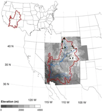
Figure 1 depicts the geographic extent of the study area and of the SNOTEL sites that were used in the model verifica-tion. The area (43◦48′N, 116◦06′W) encompasses a
model-ing domain of 1 504 800 km2. The area is rugged and
strad-dles the Continental Divide and has a mean elevation of 2203 m (σ= 517 m). The SNOTEL sites used for validation are mainly in the upper Colorado Basin. The average yearly precipitation that falls on the upper Colorado Basin, esti-mated from 39 SNOTEL stations, was 700 mm (±184 mm)
for the three water years of the study – 2006, 2007, and 2008. The area has a low (∼11 %) tree vegetation cover.
3 Model and data
SWE recorded from SNODAS and SNOTEL was compared with the SWE simulated by the UEB snowmelt model and SWE estimated from microwave imagery. In the following sections, we describe the UEB snowmelt model, model input data sets, and the results of the SWE product intercompar-isons. Because the SNODAS system assimilates most of the real-time recorded SWE data in the conterminous US, we assumed that the SNODAS SWE data were observed data. Although SNODAS SWE is the best regional-scale, spatially distributed SWE data available, we are not aware of a com-prehensive validation of the SWE estimated by the SNODAS system. The snowmelt model was run for the period Decem-ber 2005–April 2008.
3.1 Snow accumulation and ablation model
Table 1.Snowmelt model inputs, outputs, and state variables. The input includes static distributed parameters and dynamic meteorological data.
Dynamic inputs Static inputs Output fluxes State variables
Incoming shortwave rad. Elevation Latent heat flux Snow energy content Incoming longwave rad. Vegetation cover Sensible heat flux Snow water content Air temperature Vegetation height Ground heat flux Snow age
Average wind speed Soil bulk density Snow temperature Precipitation Melt advected energy Relative humidity Melt outflow flux Atmospheric pressure
by means of three state variables (snow water equivalence, snow water content, and the age of the snow surface) using a lumped representation of the snowpack as a single layer. Ta-ble 1 lists input, output, and model state variaTa-bles. By using spatially distributed meteorological fields, we assumed that we would be able to account for the snow cover heterogene-ity component caused by the variabilheterogene-ity of the precipitation and solar radiation fields.
For model parameters, we kept the values of the UEB model parameters from Tarboton and Luce (1996) un-changed, except for the snow density, which was changed from 450 to 320 kg m−3 – a value that is more
appropri-ate for the study area (Josberger et al., 1996; Molotch and Bales, 2005). To estimate model parameters, Tarboton and Luce (1996) have a calibration data set from the Central Sierra Snow Laboratory collected in the winter of 1985– 1986. Even though the model has snow redistribution capa-bility, there is no straightforward way to determine appro-priate drift factor for every modeling grid. Besides, the sizes of our modeling grids (0.05◦×0.05◦and 0.1◦×0.1◦) do not
warrant modeling snow redistribution processes that usually take place at smaller scales. Therefore, snow redistribution was not taken into account in the simulation results that are presented here.
3.2 Data
The snow energy balance model was run with inputs of air temperature, precipitation, wind speed, humidity, and radi-ation (longwave and shortwave) with a temporal resolution of 6 h time steps and spatial resolutions of 0.05◦×0.05◦and
0.1◦×0.1◦(about 5 and 10 km). Six hours is the maximum
time step that is sufficient to resolve the solar diurnal cy-cle (Tarboton and Luce, 1996). Precipitation is the most im-portant meteorological model input variable. The precipita-tion data used for the 0.05◦modeling resolution was the
Na-tional Weather Service (NWS) regional River Forecast Cen-ters (RFCs)’s Multi-sensor Precipitation Estimator (MPE) data set, where the precipitation input for the 0.1◦
resolu-tion runs was the TRMM precipitaresolu-tion estimates. In the sub-sequent paragraphs, we describe model input meteorological data and the data that were used to test simulated SWE ability
to monitor the snowpack water content through the season. Table 1 summarizes the data.
3.2.1 Meteorological data from weather forecast model
The air temperature (Ta), relative humidity (RH), direct and
diffuse solar radiation (Rs), and wind speed (U) were from
the NOAA Global Forecast System (GFS) model. To match the MPE resolution; the Ta, RH, and Rs were downscaled
from their original 0.375◦ resolution grid to a 0.05◦
reso-lution grid. The downscaling algorithms rely on the topo-graphic data to downscale the coarse weather forecasting model’s output fields to the higher resolution. To downscale the three variables, terrain geomorphometric characteristics (aspect, slope, and sky-view factor) calculated from a dig-ital elevation model (DEM) were utilized. To redistribute the solar radiation, we used the algorithms of Dozier and Frew (1990) and Dubayah and Van Katwijk (1992).Tawas
downscaled with a moist adiabatic lapse rate model (Stone and Carlson, 1979), and RH was downscaled with the re-estimatedTa.
3.2.2 Multi-sensor Precipitation Estimator (MPE)
The MPE data are made by combining data from rain gages, radars, and satellite sensors. The original format of MPE data is in the Hydrologic Rainfall Analysis Project (HRAP) grid format and has an approximate spatial resolution of 4 km. Since the radar coverage of the mountainous areas of the western US is poor (Wood et al., 2003), especially during the winter, the MPE product west of the Continental Divide is mainly made from gage reports and long-term climato-logic precipitation data (PRISM). The MPE has been oper-ational since 2002, but only data from 2005 were available for download from NOAA’s website at http://water.weather. gov/precip/download.php.
3.2.3 Tropical Rainfall Measuring Mission (TRMM)
We used TRMM precipitation data from the 3B42RT product at a 0.25◦
Table 2.Locations of the SNOTEL station where simulated SWE and MI-estimated SWE were validated.
Station Station name Lat Long Elevation ID
1 Brumley 39.08 −106.53 3231 2 Columbine Pass 38.42 −108.37 2865 3 Elk River 40.83 −106.97 2652 4 Lost Dog 40.80 −106.73 2841 5 Mccoy Park 39.60 −106.53 2890 6 Middle Fork Camp 39.78 −106.02 2725 7 Park Cone 39.82 −106.58 2926 8 Park Reservoir 39.03 −107.87 3036 9 Lone Cone 37.88 −108.18 2926 10 Elkhart Park 43.00 −109.75 2865 11 Battle Mountain 41.03 −107.25 2268 12 New Fork Lake 43.12 −109.93 2542 13 East Rim Divide 43.13 −110.20 2417 14 SandstoneRs 41.12 −107.17 2484 15 Hickerson Park 40.90 −109.95 2787 16 Trout Creek 40.73 −109.67 2901 17 Mosby Mtn 40.60 −109.88 2899 18 Lakefork #1 40.58 −110.43 3174 19 Loomis Park 43.17 −110.13 2512 20 Snider Basin 42.48 −110.52 2457 21 Kelley R. S. 42.27 −110.8 2493 22 Burro Mountain 39.87 −107.58 2865 23 Hams Fork 42.15 −110.67 2390 24 King’s Cabin 40.70 −109.53 2659 25 Lasal Mountain 38.47 −109.27 2914 26 Porphyry Creek 38.48 −106.33 3280 27 Slumgullion 37.98 −107.20 3487 28 Butte 38.88 −106.95 3097 29 Dry Lake 40.53 −106.77 2560 30 Gunsight Pass 43.37 −109.87 2993 31 Kendall R. S. 43.23 −110.02 2359 32 Stillwater Creek 40.22 −105.92 2658 33 Rock Creek 40.53 −110.68 2405 34 Indian Creek 42.30 −110.67 2873 35 Lizard Head Pass 37.78 −107.92 3109 36 Spring Creek Divide 42.52 −110.65 2743 37 El Diente Peak 37.78 −108.02 3048 38 Townsend Creek 42.68 −108.88 2652 39 McClure Pass 39.12 −107.28 2896
The microwave sensor provides the main estimates, and the IR sensors provide coverage for areas with gaps in the mi-crowave precipitation estimates. Although the TRMM 3B42 estimates are considered better than the 3B42RT product, the 3B42 is not available in real time as the 3B42RT product is. The 3B42RT products are usually posted to the TRMM Web site about 6 h after the event.
3.2.4 SWE from the microwave imagers
The SWE data sets estimated by microwave imagers that we used are from the Global Monthly EASE-Grid SWE Clima-tology (Armstrong et al., 2007). The EASE-Grid SWE data
Fig. 1.A shaded relief map of the study area and locations of the
SNOTEL sites with an outline of the Colorado Basin and western US states.
sets are monthly average values downloaded from the Na-tional Snow and Ice Data Center Distributed Active Archive Center (NSIDC, http://nsidc.org/data/), University of Col-orado at Boulder. The data are derived from the SMMR and selected SSM/Is. The EASE-Grid SWE data sets have a resolution of 25 km, about 0.25◦, but since the SSM/I
data used to produce the SWE are 19 and 37 GHz (the 19 GHz imagery has a footprint of 69 km×43 km), the
ac-tual resolution of the SWE could be coarser than the nominal 25 km. The microwave-based SWE (MI SWE) spans from December 2005 to April 2007. Only data from December to April were used in the intercomparison with the other SWE products.
3.2.5 SNOTEL
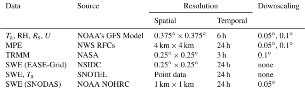
Table 3.Source and resolution of meteorological and snow data.
Data Source Resolution Downscaling
Spatial Temporal
Ta, RH,Rs,U NOAA’s GFS Model 0.375◦×0.375◦ 6 h 0.05◦, 0.1◦
MPE NWS RFCs 4 km×4 km 24 h 0.05◦, 0.1◦
TRMM NASA 0.25◦×0.25◦ 3 h 0.1◦
SWE (EASE-Grid) NSIDC 0.25◦×0.25◦ 24 h none
SWE,Ta SNOTEL Point data 24 h none
SWE (SNODAS) NOAA NOHRC 1 km×1 km 24 h 0.05◦
3.2.6 SNODAS
SNODAS is an NOAA NOHRC SWE data set (NOHRC, 2004). SNODAS is made by the assimilation of modeled SWE, remotely sensed SWE, and station-recorded SWE data. The SNODAS data set covers the conterminous US at 1 km spatial resolution and 24 h temporal resolution. Al-though we will consider hereafter the SWE as observed, we are not aware of any extensive validation done on the SNODAS SWE data sets. Because SNODAS assimilates all available observed snow data, it is difficult to validate the accuracy of the SNODAS product. Nevertheless, SNODAS has been used in several research studies and is the only pub-licly available large-scale SWE product. SNODAS data sets were downloaded from the NSIDC website (http://nsidc.org/ data). Before comparing SNODAS with other data sets, the SNODAS data were re-gridded to 0.05, 0.1, and 0.25◦
resolu-tion from the native 1 km resoluresolu-tion. Table 3 summarizes the spatial and temporal resolutions of the meteorological and snow data that were used in this study.
3.3 Performance indicators
For performance indicators, we used the percent of bias, coefficient of determination, total root mean square error (RMSE), and parameters that are based on the RMSE out-lined by Willmott (1982). Willmott (1982) decomposed the RMSE into the systematic error (RMSEs), which can be re-duced with small improvements in model parameters and in-put data, and unsystematic RMSE (RMSEu), which cannot be reduced without extensive changes in the model structure and input data. The RMSE, RMSEs, and RMSEu parameters are defined (Willmott, 1982) as
RMSE=
"
1
n
n X
i=1
(Pi −Oi)2 #1/2
,
RMSEs=
"
1
n
n X
i=1
ˆ
Pi −Oi
2 #1/2
,
RMSEu=
"
1
n
n X i=1
ˆ Pi −Pi
2 #1/2
,
wherenis the number of observations, Oi is the observed
value,Pi is the predicted value, and Pˆi=a·Oi+b. To
de-scribe how much the model underestimates or overestimates the variable of interest, the percent bias was calculated ac-cording to
Bias=100·
n P i=1
Pi −
n P i=1
Oi
n P i=1
Oi
.
4 Results and discussion
4.1 Snowmelt model meteorological inputs
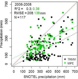
We tested the precipitation values reported by MPE and TRMM by comparing them to the precipitation values recorded at the 39 SNOTEL stations shown in Fig. 1. By comparing gridded data of varying spatial scales and point data, there should not be an expectation of perfect agreement even if both data are correct. We compared precipitation to-tals accumulated in the snow accumulation/ablation periods of the three years of the simulation period – 1 January 2006– 30 April 2006, 1 January 2007–30 April 2007, and 1 Jan-uary 2008–28 April 2008 (d.f. = 115). Both MPE and TRMM were negatively biased against SNOTEL precipitation as il-lustrated in Fig. 2; on average the percent bias of the MPE per season for the 39 locations was−26 % with a mean and
standard deviation of−84±110 mm, and for the TRMM the bias was−51 % (−164±124 mm). The correlation between the MPE and TRMM was even lower than the one the two data sets had with SNOTEL data (r= 0.53). Higher
propor-tions of the precipitation differences with SNOTEL sets were systematic errors for both the TRMM (86 % of RMSE) and the MPE data sets (77 % of RMSE), which means the data could be improved with simpler correction schemes.
Fig. 2.Scatterplots of the total precipitation recorded at 39 SNO-TEL sites for the periods of 1 January 2006–30 April 2006, 1 Jan-uary 2007–30 April 2007, and 1 JanJan-uary 2008–28 April 2008 com-pared with precipitation estimates for the same locations from MPE (black) and TRMM (green).
magnitude of the discrepancy between some of the SNOTEL station-recorded precipitation and the MPE suggests that the MPE estimation needs to be improved. Our results on the bias direction, being inclined for underestimation, are in line with what Habib et al. (2009) observed when they weighted precipitation values from MPE against rain-gage-recorded precipitation.
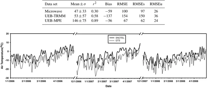
The GFS daily meanTaextracted from grid-cells was
com-pared to SNOTEL-recorded Ta from the 39 stations. The
GFSTa was created by averaging four 6 hTa. The
compar-ison period was the same as the precipitation evaluation pe-riod – winter and spring – when theTa influences the snow
process. The elevation at the 39 sites ranges from 2268 to 3487 m. Figure 3 shows the plots of the average daily GFS-and SNOTEL-recordedTa for the 39 sites for the three
sea-sons. GFSTaseasonally matches the SNOTEL-recordedTa
(Fig. 3). TheTaof both GFS and SNOTEL were significantly
correlated (R2= 0.61, d.f. = 171), but the GFSTawere
neg-atively biased versus theTa recorded at the SNOTEL sites.
The bias between GFS and SNOTELTa was not correlated
with elevation (Fig. 4). The negative bias of the GFSTa is
counterintuitive given that the SNOTEL sites are usually lo-cated at higher elevations than the surrounding terrain. The presence of a negative bias within all elevation bands sug-gests that the elevation correction applied to the original GFS data was not the cause of the biases, but a systematic GFS underestimation bias. Others have reported similar results of negative biases of weather forecast model air temperature in the western US during the winter months (Pan et al., 2003).
4.2 Spatial intercomparisons of the SWE data sets
The SWE grids simulated with the UEB model and the SWE grids estimated from MI were compared against SWE from SNOTEL and SNODAS. While the SWE from the UEB sim-ulations and the SNODAS system had only a few grids with missing data (grids over water bodies), the SWE estimated from the MI data sets has a high number of pixels with missing data. For example, MI-estimated SWE had missing data in 40 % of the area for February 2007 (Fig. 5). The evaluation of the SWE was done at the grids correspond-ing with the sites of the 39 SNOTEL sites shown in Fig. 1. The SNODAS grids used in the comparisons were upscaled from their native 1 km (∼0.01◦) resolution to grids with 0.05,
0.10, and 0.025◦ resolution. Statistical indexes (correlation
coefficients, percent biases, RMSE, RMSEs, and RMSEu) were calculated at each of the 39 validation sites between the SNODAS SWE and MI- and UEB-produced SWE. Ad-ditionally, to give a contextual frame-of-reference, the SWE products were compared to the SWE recorded at the 39 sites by the SNOTEL system.
The average monthly SWE value recorded at the SNO-TEL sites was 259±96 mm (mean±standard deviation) and
240±98 mm for the periods January 2006–April 2008 (UEB
simulations period) and January 2006–April 2007 (the pe-riod where MI-estimated SWE was available), respectively. Of the 39 sites, the SWEs simulated with the UEB were sig-nificantly correlated with the SNODAS SWE (p= 0.05) in
38 and 25 sites for the MPE and TRMM precipitation, re-spectively (Fig. 7a). The SWE estimated from MI was not significantly correlated (p= 0.05) with the SNODAS SWE at 12 sites (Fig. 7a). The correlation between the SWE prod-ucts and the SNOTEL recorded SWE was significant at 39, 27, and 2 sites for the UEB-MPE, UEB-TRMM, and MI-SWE products, respectively (Fig. 7b).
Figure 8a–f shows linear and box plots of the three SWE products contrasted with concurrent SNOTEL and SNODAS SWE. The MI-estimated SWE consistently underestimates the SWE depicted by the SNODAS or the SNOTEL (Fig. 8c). The SWE simulated with the UEB model forced with TRMM data for precipitation also consistently underpredicted the SWE most of the time (Fig. 8b). The SWE modeled with UEB driven with the MPE data was in good agreement with the SNODAS and SNOTEL SWE values, except for one lo-cation that had an extremely large SWE value (Fig. 8d).
Table 4.Statistical summary of the comparison between the SWE products and the SNOTEL data sets. The last row is the statistics summary of comparison between the 0.05◦resolution SNODAS and the point SNOTEL SWE.
Data set Mean±σ r2 Bias RMSE RMSEs RMSEu
Microwave 47±33 0.20 −167 % 184 182 28 UEB-TRMM 53±57 0.46 −186 % 203 199 41 UEB-MPE 146±75 0.87 −37 % 107 102 32 SNODAS 202±98 0.96 −37 % 43 39 18
Table 5.Statistical summary of the evaluation of SWE products compared to the SNODAS product. The SNODAS product compared to
each product had the spatial and temporal resolution as the products (0.05, 0.10, and 0.25◦resolution; daily or monthly).
Data set Mean±σ r2 Bias RMSE RMSEs RMSEu
Microwave 47±33 0.30 −59 100 97 26 UEB-TRMM 53±57 0.58 −137 154 150 36 UEB-MPE 146±75 0.89 −56 67 62 24
1/1/2006 2/1/2006 3/1/2006 4/1/2006
A
ir
T
em
p
er
atu
re(
oC)
-30 -20 -10 0 10 20
Date
12/1/2006 1/1/2007 2/1/2007 3/1/2007 4/1/2007
SNOTEL GTS
12/1/2007 1/1/2008 2/1/2008 3/1/2008 4/1/2008
Fig. 3.Average daily forecasted GFS air temperature (dotted) and SNOTEL-recorded daily average temperature (solid line) at the 39
SNO-TEL sites. GFS’s air temperatures were extracted from 0.05◦ resolution grids and an average of the 06:00, 12:00, 18:00 UTC, and the
following day 00:00 UTC forecasts.
Fig. 4.Bias of the GFS average daily air temperature from the air
temperature recorded at the SNOTEL sites and the sites’ elevations.
and f). We think that the lower variability of the TRMM-simulated SWE was in part due to the sub-optimal model grid resolution for modeling the snow accumulation/ablation pro-cesses in the study area (Artan et al., 2000; Blöschl, 1999) and the low accuracy of the TRMM 3B42RT product (see Fig. 2).
Tables 4 and 5 summarize the statistical indices of the SWE comparisons. Of the three SWE products, the SWE simulated with UEB when forced with NOAA’s MPE precip-itation was the best performer. The TRMM-simulated SWE and MI-estimated SWE are not adept as site specific snow-pack monitoring tools.
Fig. 5.Average SWE for February 2007 predicted with the distributed UEB model, microwave imagery, and SNODAS. Over 40 % of the area had missing data for the SWE data set estimates from the microwave imagery.
SNOTEL Locations
0 10 20 30 40
Correlat
ion
Coef
ficient
-1.0 -0.5 0.0 0.5 1.0
SWE MPE SWE-TRMM SWE-MI
SNOTEL Locations
0 10 20 30 40
-1.0 -0.5 0.0 0.5 1.0
SWE MPE SWE-TRMM SWE-MI
(A) (B)
Fig. 6.Correlation coefficients between the average seasonal(A)SNODAS SWE at various grid resolutions and(B)the SWE recorded by
the SNOTEL site at 39 sites in the upper Colorado Basin with the SWE estimate products from the MI imagery and UEB simulations.
SWE at lower elevation terrains. All three SWE products had the lowest skills in the southwestern part of the study area.
Among the three SWE data sets we evaluated to reproduce SWE values seen in the SNODAS and SNOTEL data sets, the performance of the MI-estimated SWE was the worst in most of the correlation metrics. The MI SWE had the lowest cor-relation with the SNODAS and SNOTEL SWE. Both the MI – estimated SWE and UEB-TRMM – simulated SWE had relatively large systematic errors. Both products also lack the
SNOTEL Station ID
0 10 20 30 40
S
W
E
(m
m)
0 200 400 600 800
Snotel Snodas - 0.250
Microwave - SWE
SNOTEL Station ID
0 10 20 30 40
0 200 400 600 800
Snotel Snodas - 0.10
UEB-TRMM
SNOTEL Station ID
0 10 20 30 40
0 200 400 600 800
Snotel Snodas - 0.050
UEB-MPE
SNOTEL SNODAS-0.25 Microwave
S
W
E
(m
m)
0 100 200 300 400 500 600
SNOTEL SNODAS-0.1 UEB-TRMM 0
100 200 300 400 500 600
SNOTEL SNODAS-0.05 UEB-MPE 0
100 200 300 400 500 600
(D) (F)
(B)
(A) (C) (E)
Fig. 7.Average SWE from SNOTEL and SNODAS for the winter and spring months compared with SWE estimated from(A)MI,(C)SWE
predicted with UEB when driven with TRMM precipitation, and(E)UEB forced with MPE precipitation. The SWE simulated with the UEB is for the period January 2006–April 2008, excluding the months from June to November.(B, D, F)are box plots of the data in the first three graphs.
678 679
Elevation(m)
2200 2400 2600 2800 3000 3200 3400 3600
C
or
relation
C
oef
fic
ient
-1.0 -0.8 -0.6 -0.4 -0.2 0.0 0.2 0.4 0.6 0.8 1.0
(A)
Elevation(m)
2200 2400 2600 2800 3000 3200 3400 3600
C
or
relation
C
oef
fic
ient
-1.0 -0.5 0.0 0.5 1.0
(B)
Elevation(m)
2200 2400 2600 2800 3000 3200 3400 3600
C
or
relation
C
oef
fic
ient
-1.0 -0.5 0.0 0.5 1.0
(C) R2 = 0.02
R2 = 0.12 R2 = 0.01
Fig. 8.Relationships between elevations and correlation between the three SWE products and SNODAS SWE plotted at the SNOTEL
Months Since Aug 2005
Aug Feb Aug Feb Aug Feb Aug
SW
E (
m
m
)
0 100 200 300 400 500
SNOTEL Microwave SNODAS 0.25o
Months Since Aug 2005
Aug Feb Aug Feb Aug Feb Aug
SW
E (
m
m
)
0 100 200 300 400 500
SNOTEL UEB-TRMM SNODAS 0.1o
Months Since Aug 2005
Aug Feb Aug Feb Aug Feb Aug
SW
E (
m
m
)
0 100 200 300 400 500
SNOTEL UEB-MPE SNODAS 0.05o
(A) (B)
(C)
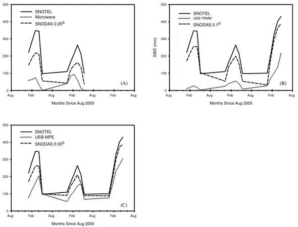
Fig. 9.Time series plots of averaged SWE (at the 39 SNOTEL sites) from SNOTEL and SNODAS and(A)the microwave imagers,(B)
sim-ulated with the UEB model with TRMM precipitation, and(C)modeled with UEB model and MPE precipitation.
SWE from microwave imagery. The low random error com-ponent, once the sources of the errors are fully known, should make possible the improvement of the UEB-TRMM and Mi-estimated SWE product.
4.3 Temporal intercomparisons of the SWE data sets
The average SWE value at the 39 SNOTEL sites was calcu-lated at every time step (16 months of data for all products except the MI-estimated SWE, which only had 11 months of data available) for the simulated and observed SWE data sets. Figure 9a–c shows the time series plots of the evolution through the season of the average SWE in the study area from SNOTEL, SNODAS, estimated from MI, and simulated by the UEB. All of the SWE products displayed a similar evalu-ation of the SWE temporal pattern. The SWE estimated from the MI showed (Fig. 9a) an earlier start of the melt season than either SNODAS or SNOTEL, but the snowpack simu-lated with the UEB model (Fig. 9b and c) showed a later start of the melt season than SNODAS. Although the SWE esti-mated from the MI has a monthly time step that makes it dif-ficult to accurately quantify the exact date of the start of the melt season, prediction of the start of the melt season of one month earlier by the MI will decrease the usefulness of the SWE-MI product for monitoring purposes. The SNODAS
SWE start of the melt period for two seasons (2005/2006 and 2006/2007) was about two weeks earlier than SNOTEL’s.
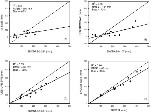
Figure 10a–d presents the linear relationships between the average monthly values of the SWE products. The SWE es-timated from the MI was not significantly correlated with the SNODAS SWE (Fig. 10a). But the SWE simulated with the UEB models was in good agreement with the SNODAS-estimated SWE (Fig. 10b and c) with a clear linear relation-ship. The UEB-MPE-simulated SWE mostly captured the SNODAS SWE evolution through the season. Figure 10d shows the average area-wide SWE from the SNODAS and SNOTEL data sets. The striking feature of Fig. 10d is the great agreement between the two products in the three years of the comparison (16 months).
The later start of the melt season seen in the plots of UEB-simulated SWE (Fig. 9b and c) was due to the negative bias seen in model input air temperature (Fig. 4) and elucidates the effects of the errors in the input meteorological data on the UEB-simulated SWE. To investigate the influence of the bias of the input air temperature, we re-ran the UEB-MPE by increasing the air temperature from GFS by 2◦
SNODAS-0.05o (mm)
0 100 200 300 400 500
UE B -M P E S W E ( m m ) 0 100 200 300 400 500 SNODAS-0.10o (mm)
0 100 200 300 400 500
UE B -T RM M S W E ( m m ) -100 0 100 200 300 400 500 SNODAS-0.25o (mm)
0 100 200 300 400 500
M I S W E ( m m ) 0 100 200 300 400 500 SNOTEL (mm)
0 100 200 300 400 500
S NODA S S W E ( m m ) 0 100 200 300 400 500
R2 = 0.89 RMSE = 67 mm Bias = -28%
R2 = 0.58 RMSE = 154 mm Bias = -72% R2
= 0.3 RMSE = 100 mm Bias = -65%
R2 = 0.96 RMSE = 43 mm Bias = -15%
(A) (B)
(C) (D)
Fig. 10.Averaged SWE (at the 39 SNOTEL sites) from the SNODAS and the(A)SWE estimated from the microwave imagers for December–
May between January 2006 and April 2007;(B)SWE from the DisUEB with TRMM precipitation, and(C)DisUEB with MPE for Jan-uary 2006–April 2008.(D)Average SWE of the SNODAS and SNOTEL data sets for the period January 2006–April 2008.
SNODAS-0.05o (mm)
0 100 200 300 400 500
U EB -M PE S W E (m m ) 0 100 200 300 400 500 SNODAS-0.05o (mm)
0 100 200 300 400 500
U EB -M PE S W E (m m ) 0 100 200 300 400 500
R2 = 0.89 RMSE = 64 mm Bias = -37%
R2 = 0.94 RMSE = 68 mm Bias = -43%
Fig. 11.Scatterplots of average daily SWE (at the 39 SNOTEL sites) from the SNODAS and the(A)SWE from simulated with UEB and MPE
precipitation and the original GFS air temperature for January 2006–April 2008, and(B)SWE simulated with UEB and MPE precipitation and the original GFS air temperature increased by 2◦C.
starts earlier and with a faster rate of melt, which improves the performance of the simulated SWE.
Most of the time, the UEB model underestimated SWE compared to the SWE values recorded at the SNOTEL sta-tions and SNODAS. Our findings, on the underestimation of the simulated SWE, are consistent with the findings of other research on the underestimation biases of simulated SWE
agreement between the SNODAS- and SNOTEL-recorded SWE was marginal. Although the TRMM-simulated SWE had low quantitative skills to predict snow water content it nevertheless had good qualitative skills to predict snow water given the high correlation it exhibited when compared with SNODAS time series data. The better correlation between SWE simulated with UEB-TRMM and SWE from SNODAS and SNOTEL when time series basin-wide values were used is due to seasonality of the precipitation occurrence being captured by TRMM.
From a practical point of view, we found the MI-estimated SWE and SWE simulated from TRMM data sets to be un-reliable sources for mapping SWE in the study area and to have a large underestimation bias compared with the SNO-TEL SWE or the SWE estimated by the SNODAS system. Our results on the negative biases of the MI-estimated SWE are different from what Mote et al. (2003) reported. Mote et al. (2003) found that SWE estimated from SSM/I overpre-dicted during the melting period for five sites in the northern Great Plains.
5 Conclusions
We presented a distributed snow accumulation and abla-tion model that is built on the UEB model that uses data from weather forecast models as forcing input. Besides the weather forecast model (GFS) data, the snowmelt model was forced with two precipitation data sets: the NWS MPE and the TRMM precipitation estimates. The model was run at a 0.050 and 0.100◦ resolution for the MPE and TRMM,
respectively. We compared model-simulated SWE and MI-estimated SWE with co-located SWE data sets recorded by the SNOTEL network or estimated by the SNODAS system. The SWE simulated by the UEB model was strongly corre-lated with the SWE estimated by SNODAS (R2= 0.58 and
R2= 0.89 for model input precipitation as TRMM and MPE, respectively) and the SWE recorded by SNOTEL (R2= 0.46 andR2= 0.87) when the seasonal average SWE values were compared. The MI-estimated SWE was significantly corre-lated with the SNOTEL and not correcorre-lated with the SNODAS SWE product (R2of 0.3 and 0.2, respectively).
Both of the UEB-simulated and MI-estimated SWEs un-derestimated the SWE reported by the SNOTEL or SNODAS systems. The MI-estimated and the UEB-simulated SWE underestimated the SWE values seen in the SNOTEL and SNODAS data sets and lacked a discernable variability be-tween sites seen in the SNOTEL and SNODAS SWE data and were found to be unreliable sources for mapping SWE in the study area. In the future, we will evaluate the effects of the parameterization of the snow albedo on the snowmelt processes by using remotely sensed snow albedo as input to the model. Notwithstanding their experimental nature, sev-eral snow albedo products with near-global coverage are now becoming available. Another area of future research is
quantifying the propagations of uncertainty of the input me-teorological data to the snow model output variables.
Acknowledgements. The authors would like to thank
Gabriel Senay, Lei Ji, and Thomas Adamson for helpful comments on an early draft of the manuscript. We also would like to thank two anonymous referees for their constructive comments, which led to substantial improvements in the manuscript. The work of Guleid Artan was performed under USGS contract G13PC00028.
Edited by: A. Langousis
References
Armstrong, R. L., Brodzik, M. J., Knowles, K., and Savoie, M.: Global monthly EASE-Grid snow water equivalent climatology, National Snow and Ice Data Center, Digital media, Boulder, CO, 2007.
Artan, G. A., Neale, C. M. U., and Tarboton, D. G.: Characteristic length scale of input data in distributed models: Implications for modeling grid size, J. Hydrol., 227, 128–139, 2000.
Bales, R. C., Dressler, K. A., Imam, B., Fassnacht, S. R., and Lampkin, D.: Fractional snow cover in the Colorado and Rio Grande basins, 1995–2002, Water Resour. Res., 44, W01425, doi:10.1029/2006WR005377, 2008.
Blöschl, G.: Scaling issues in snow hydrology, Hydrol. Process., 13, 2149–2175, doi:10.1029/2006WR005377, 1999.
Carroll, S. S.: Modeling measurement errors when estimating snow water equivalent, J. Hydrol., 172, 247–260, 1995.
Chen, C. T., Nijssen, B., Guo, J., Tsang, L., Wood, A. W., Hwang, J. N., and Lettenmaier, D. P.: Passive microwave remote sensing of snow constrained by hydrological simulations, IEEE T. Geosci. Remote, 39, 1744–1756, 2001.
Cline, D. W., Bales, R. C., and Dozier, J.: Estimating the spatial distribution of snow in mountain basins using remote sensing and energy balance modeling, Water Resour. Res., 34, 1275–1285, 1998.
Daly, S. F., Davis, R., Ochs, E., and Pangburn, T.: An approach to spatially distrubuted snow modelling of the sacramento and San Joaquin basins, California, Hydrol. Process., 14, 3257–3271, 2000.
Dong, J., Walker, J. P., and Houser, P. R.: Factors affecting remotely sensed snow water equivalent uncertainty, Remote Sens. Envi-ron., 97, 68–82, 2005.
Dozier, J. and Frew, J.: Rapid calculation of terrain parameters for radiation modeling from digital elevation data, IEEE T. Geosci. Remote, 28, 963–969, 1990.
Dressler, K. A., Leavesley, G. H., Bales, R. C., and Fassnacht, S. R.: Evaluation of gridded snow water equivalent and satellite snow cover products for mountain basins in a hydrologic model, Hy-drol. Process., 20, 673–688, 2006.
Dubayah, R. and Van Katwijk, V.: The topographic distribution of annual incoming solar radiation in the Rio Grande River Basin, Geophys. Res. Lett., 19, 2231–2234, 1992.
Habib, E., Larson, B. F., and Graschel, J.: Validation of NEXRAD multisensor precipitation estimates using an experimental dense rain gauge network in south Louisiana, J. Hydrol., 373, 463–478, 2009.
Janowiak, J. E., Joyce, R. J. and Yarosh, Y.: A real-time global half-hourly pixel-resolution infrared dataset and its applications, B. Am. Meteorol. Soc., 82, 205–217, 2001.
Josberger, E. G., Gloersen, P., Chang, A., and Rango, A.: The ef-fects of snowpack grain size on satellite passive microwave ob-servations from the Upper Colorado River Basin, J. Geophys. Res.-Oceans, 101, 6679–6688, 1996.
Joyce, R. J., Janowiak, J. E., Arkin, P. A., and Xie, P.: CMORPH: A method that produces global precipitation estimates from passive microwave and infrared data at high spatial and temporal resolu-tion, J. Hydrometeorol., 5, 487–503, 2004.
Kelly, R. E., Chang, A. T., Tsang, L., and Foster, J. L.: A prototype AMSR-E global snow area and snow depth algorithm, IEEE T. Geosci. Remote, 41, 230–242, 2003.
Koivusalo, H. and Heikinheimo, M.: Surface energy exchange over a boreal snowpack: Comparison of two snow energy balance models, Hydrol. Process., 13, 2395–2408, 1999.
Molotch, N. P. and Bales, R. C.: Scaling snow observations from the point to the grid element: Implications for observation network design, Water Resour. Res., 41, 1–16, 2005.
Molotch, N. P. and Bales, R. C.: SNOTEL representativeness in the Rio Grande headwaters on the basis of physiographics and remotely sensed snow cover persistence, Hydrol. Process., 20, 723–739, 2006.
Mote, T. L., Grandstein, A. J., Leathers, D. J., and Robinson, D. A.: A comparison of modeled, remotely sensed, and measured snow water equivalent in the northern Great Plains, Water Resour. Res., 39, 1209, doi:10.1029/2002WR001782, 2003.
NOHRC – National Operational Hydrologic Remote Sensing Cen-ter: Snow Data Assimilation System (SNODAS) data products at NSIDC, National Snow and Ice Data Center, Boulder, Colorado, USA, 2004.
Pan, M., Sheffield, J., Wood, E. F., Mitchell, K. E., Houser, P. R., Schaake, J. C., Robock, A., Lohmann, D., Cosgrove, B., Duan, Q., Luo, L., Higgins, R. W., Pinker, R. T., and Tarpley, J. D.: Snow process modeling in the North American Land Data As-similation System (NLDAS): 2. Evaluation of model simulated snow water equivalent, J. Geophys. Res.-Atmos., 108, 8850, doi:10.1029/2003JD003994, 2003.
Robinson, D. A. and Kukla, G.: Maximum surface albedo of sea-sonally snow-covered lands in the Northern Hemisphere, J. Clim. Appl. Meteorol., 24, 402–411, 1985.
Robinson, D. A., Dewey, K. F., and Heim Jr., R. R.: Global snow cover monitoring: an update, B. Am. Meteorol. Soc., 74, 1689– 1696, 1993.
Schmugge, T. J., Kustas, W. P., Ritchie, J. C., Jackson, T. J., and Rango, A.: Remote sensing in hydrology, Adv. Water Resour., 25, 1367–1385, 2002.
Schulz, O. and de Jong, C.: Snowmelt and sublimation: field ex-periments and modelling in the High Atlas Mountains of Mo-rocco, Hydrol. Earth Syst. Sci., 8, 1076–1089, doi:10.5194/hess-8-1076-2004, 2004.
Serreze, M. C., Clark, M. P., Armstrong, R. L., McGinnis, D. A., and Pulwarty, R. S.: Characteristics of the western United States snowpack from snowpack telemetry (SNOTEL) data, Water Re-sour. Res., 35, 2145–2160, 1999.
Stone, P. and Carlson, J.: Atmospheric lapse rate regimes and their parameterization, J. Atmos. Sci., 36, 415–423, 1979.
Sun, C., Neale, C. M. U., and McDonnell, J. J.: Snow wetness esti-mates of vegetated terrain from satellite passive microwave data, Hydrol. Process., 10, 1619–1628, 1996.
Tarboton, D. G. and Luce, C. H.: Utah Energy Balance Snow Accu-mulation and Melt Model (UEB): Computer model technical de-scription and users guide, Utah Water Research Laboratory and USDA Forest Service Intermountain Research Station, Logan, Utah, 64 pp., 1996.
Tekeli, A. E., Akyürek, Z., ¸Sorman, A. A., ¸Sensoy, A., and ¸Sorman, A. Ü.: Using MODIS snow cover maps in modeling snowmelt runoff process in the eastern part of Turkey, Remote Sens. Envi-ron., 97, 216–230, 2005.
Tian, Y., Peters-Lidard, C. , Choudhury, B., and Garcia, M.: Mul-titemporal analysis of TRMM-based satellite precipitation prod-ucts for land data assimilation applications, J. Hydrometeorol., 8, 1165–1183, 2007.
Watson, F. G. R., Newman, W. B., Coughlan, J. C., and Garrott, R. A.: Testing a distributed snowpack simulation model against spatial observations, J. Hydrol., 328, 453–466, 2006.
Willmott, C. J.: Some comments on the evaluation of model perfor-mance, B. Am. Meteorol. Soc., 63, 1309–1313, 1982.
Wood, V. T., Brown, R. A., and Vasiloff, S. V.: Improved detec-tion using negative elevadetec-tion angles for mountaintop WSR-88Ds, Part II: Simulations of the three radars covering Utah, Weather Forecast., 18, 393–403, 2003.