A METHOD FOR QUALITY POWER PROVIDER TO OPERATE IN DISTORTED SUPPLY CONDITION

18

A METHOD FOR QUALITY POWER PROVIDER TO

OPERATE IN DISTORTED SUPPLY CONDITION

1

K.CHANDRASEKARAN, 2K.S.RAMA RAO

1

PhD student, Electrical and Electronic Department, Universiti Teknologi PETRONAS, Malaysia

2

Assoc. Prof., Electrical and Electronic Department, Universiti Teknologi PETRONAS, Malaysia

E-mail: chandthi@streamyx.com, ksramarao@petronas.com.my

ABSTRACT

Power Quality is a major concern within power industry and consumers. Poor quality of supply will affect the performance of customer equipment such as computers, microprocessors, adjustable speed drives, power electronic controllers, life saving equipment in hospitals, etc. and result in heavy financial losses to customers due to loss of production or breakdown in industries or loss of life in a hospital. The two major power quality disturbances are voltage sag and harmonic distortion. In this paper, a Quality Power Provider (QPP) based on voltage source inverter is modeled by simulation to compensate the power quality disturbances such as voltage sag and voltage harmonics in the distorted supply condition. The phase locked loop (PLL) is an important control unit of the QPP control scheme. To obtain accurate phase information and frequency of the input supply, the dqPLL method has been proposed. Simulation results based on MATLAB and PSCAD software are presented to verify the performance of the proposed QPP. QPP has improved the quality of power supply at the sensitive load end.

Keywords:Voltage Sag, Harmonics, PLL, Dqpll, Double Frequency Component.

1. INTRODUCTION

The main causes of voltage disturbances in power system are due to insulation failure, tree falling, bird contact, lightning or a fault on an adjacent feeder. These disturbances may be in the form of voltage sags, swells, interruptions and harmonics. However, harmonic distortion in power system is caused by non-linear loads [1]. Voltage disturbances will cause problems to the industrial equipments ranging from malfunctioning of equipments to complete plant shutdowns [2]. A QPP is designed based on three single-phase IGBTs H-bridge inverters which are connected to the distribution system by three injection transformers. The QPP is connected at the point of common coupling in series with the sensitive load and in parallel with a three-phase uncontrolled bridge rectifier acting as a non-linear load. The PLL is an important control unit used with the QPP, to obtain the phase and frequency information of the input supply voltage. The PLL is used to generate unit sine and cosine signals to compute the feedback and modulating control signals. It is difficult for the PLL to generate these unit vectors when the input supply voltage is distorted like unbalanced, presence of

harmonics, voltage sag and phase jump. The PLL has to track the phase information accurately under distorted supply conditions. Some methods have been proposed in the literature as in [3][4][5] for accurate phase angle tracking in distorted supply conditions. Each method has its own drawbacks. In this paper, the dqPLL method based on the dq method is developed to improve the performance of the PLL and QPP under distorted supply conditions. The performance of QPP is investigated in balanced and unbalanced fault conditions, harmonics distortion, and balanced and unbalanced fault conditions together with harmonics. Simulation results indicate an improved performance by the QPP.

2. MATHEMATICAL MODELING OF PLL

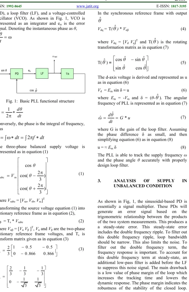
19 (PD), a loop filter (LF), and a voltage-controlled oscillator (VCO). As shown in Fig. 1, VCO is represented as an integrator and err is the error

signal. Denoting the instantaneous phase as θ,

ω =

dt dθ

PD LF 1/s

err

sin θ

cos θˆ

ωest

Fig. 1: Basic PLL functional structure

dt dθ

f ∗

π =

2 1

Conversely, the phase is the integral of frequency, thus

∫

ω

∗

=

∫

π

∗

=

dt

f

dt

θ

2

The three-phase balanced supply voltage is represented as in equation (1)

⎥ ⎥ ⎥ ⎥ ⎥ ⎥

⎦ ⎤

⎢ ⎢ ⎢ ⎢ ⎢ ⎢

⎣ ⎡

π +

π − =

) 3 2 cos(

) 3 2 cos(

cos

m sabc

θ θ

θ

V

V (1)

where Vsabc = [Vsa, Vsb, Vsc]T

Transforming the source voltage equation (1) into stationary reference frame as in equation (2),

Vαβ = Ts * Vsabc (2)

where Vαβ = [VαVβ ]T, Vα and Vβ are the two-phase

stationary reference frame voltages, and Ts is

transform matrix given as in equation (3)

⎥ ⎦ ⎤ ⎢

⎣ ⎡

−

− −

=

866 . 0 866 . 0 0

5 . 0 5

. 0 1 3 2

T_s (3)

or

⎥ ⎥ ⎥ ⎥

⎦ ⎤

⎢ ⎢ ⎢ ⎢

⎣ ⎡

−

− −

=

3 1 3 1 0

3 1 3

1 3 2

Ts

In the synchronous reference frame with output

θ

ˆ

Vdq = T(

θ

ˆ

) * Vαβ (4)

where Vdq = [Vd Vq]T and T(

θ

ˆ

) is the rotating

transformation matrix as in equation (7)

T(

θ

ˆ

) =

⎥ ⎥ ⎦ ⎤ ⎢

⎢ ⎣

⎡ ₋

θ θ

θ θ

ˆ cos ˆ

sin

ˆ sin ˆ cos

(5)

The d-axis voltage is derived and represented as u as in equation (6)

Vd = Em sin δ = u (6)

where Em = -Vm and δ = (θ-

θ

ˆ

). The angular

frequency of PLL is represented as in equation (7)

u G dt

θ

d

ωˆ = ˆ = * (7)

where G is the gain of the loop filter. Assuming the phase difference δ as small, and then simplifying equation (6) as in equation (8)

u = ≈Emδ (8)

The PLL is able to track the supply frequency ω and the phase angle θ accurately with properly design loop filter.

3. ANALYSIS OF SUPPLY IN

UNBALANCED CONDITION

20 Normally, the phase margin should be around 60 degrees [6]. This means that the frequency at which the open and close loop gains meet, the phase angle is -120 degrees. That is, (-1200 -(-1800)) equals 60 degrees. A phase margin of 600 allows fastest time when attempting to follow step input. Also, if the input supply voltage is distorted and unbalanced in a 50 Hz system, a ripple frequency of 100 Hz will appear in the d and q axis of the dq method along with the dc quantities which will result in error estimation of θ.

4. NEW PROPOSED dqPLL TECHNIQUE

The unbalanced supply phase voltages in symmetrical components are represented as in equation (9) ⎥ ⎥ ⎥ ⎦ ⎤ ⎢ ⎢ ⎢ ⎣ ⎡ + ⎥ ⎥ ⎥ ⎦ ⎤ ⎢ ⎢ ⎢ ⎣ ⎡ + ⎥ ⎥ ⎥ ⎦ ⎤ ⎢ ⎢ ⎢ ⎣ ⎡ = ⎥ ⎥ ⎥ ⎦ ⎤ ⎢ ⎢ ⎢ ⎣ ⎡ = − − − + + + c0 b0 a0 c b a c b a c b a sabc V V V V V V V V V V V V

V (9)

Using αβ transform, Tαβ

abc

αβ _V T V

V V _αβ β α ₌ ⎥ ⎦ ⎤ ⎢ ⎣ ⎡

= (10)

⎥ ⎥ ⎥ ⎦ ⎤ ⎢ ⎢ ⎢ ⎣ ⎡ + ⎥ ⎥ ⎥ ⎦ ⎤ ⎢ ⎢ ⎢ ⎣ ⎡ + ⎥ ⎥ ⎥ ⎦ ⎤ ⎢ ⎢ ⎢ ⎣ ⎡ = − − − + + + c0 b0 a0 αβ c b a αβ c b a αβ

αβ T T T

V V V V V V V V V

V (11)

representing ) 3 2π sin( ; ) 3 2π sin( ; sin ) 3 2π sin( ; ) 3 2π sin( ; sin -c -b -a c b a − = + = = + = − = = − − − − + + + + + + + + + θ V V θ V V θ V V θ V V θ V V θ V V then

⎥

⎥

⎦

⎤

⎢

⎢

⎣

⎡

+

−

+

=

⎥

⎦

⎤

⎢

⎣

⎡

=

− − + + − − + +

θ

V

θ

V

θ

V

θ

V

V

V

V

cos

cos

sin

sin

αβ β α (12) performing

dq Transform, Tdq (

θ

ˆ

) on αβ

⎥ ⎥ ⎦ ⎤ ⎢ ⎢ ⎣ ⎡ + + − − + + − = ⎥ ⎦ ⎤ ⎢ ⎣ ⎡ + − + ⎥ ⎥ ⎦ ⎤ ⎢ ⎢ ⎣ ⎡ − = ⎥ ⎦ ⎤ ⎢ ⎣ ⎡ + − + = = − − + + − − + + − − + + − − + + − − + + − − + + αβ ) ˆ ( cos ) ˆ ( cos ) ˆ ( sin ) ˆ ( sin cos cos sin sin ˆ cos ˆ sin ˆ sin ˆ cos cos cos sin sin ) ˆ ( T ) ˆ ( T dq dq dq θ θ V θ θ V θ θ V θ θ V θ V θ V θ V θ V θ θ θ θ θ V θ V θ V θ V θ V θ V (13)

The estimated phase angle =

θ

ˆ

Assuming, that the PLL successfully track the

phase at

θ

ˆ

=

θ

₋

=

θ

₊ , then

⎥

⎥

⎦

⎤

⎢

⎢

⎣

⎡

+

−

=

+ − + + −

θ

V

V

θ

V

V

ˆ

2

cos

ˆ

2

sin

dq (14)

+

θ

ˆ

2

is the double frequency, to be eliminated.

Ideally it is necessary to obtain

⎥

⎦

⎤

⎢

⎣

⎡

−

=

+

V

V

_dq

0

To eliminate the double frequency component, a new technique is introduced. An all pass function is used to introduce + 900 shift on the d-q values to eliminate the double frequency component. This is implemented with the proposed dqPLL schematic circuit as shown in Fig. 2.

abc to dq Vsa Vsb Vsc Vd Vq APF + 900

APF + 900

V- cos 2θ+

-V+ COS -V- sin 2θ+ 0

0

-V+ + -+ + -+ + -kp

ki/s + + -ω + θˆ θˆ -V- sin 2θ+

Fig. 2: Proposed dqPLL

An evaluation of the synchronization algorithms described above is explained in the following example: Consider a simulation with SLGF voltage sag of 20 %, the unbalanced supply voltage as Vsa = 184 V, Vsb = 220 V and

21 parameters of the dqPLL are adjusted as kp = 1.536 and ki = 272, where kp is proportional

gain and ki is integral time constant.

Th proposed technique is tested in PSCAD and in MATLAB / SIMULINK. The simulation results are discussed in section 7.

5. TRANSIENT ANALYSIS OF PLL

The stability condition of the PLL is obtained by investigating the PLL transfer function. The second-order transfer function of PLL linearized model is 2 n n 2 2 n n

s

2

s

s

2

)

s

(

)

s

(

ˆ

ω

+

ζω

+

ω

+

ζω

=

θ

θ

(15)

Let the input θ(t) be a unit step, u(t), so that

θ(s) = 1/s, Therefore,

⎟⎟

⎠

⎞

⎜⎜

⎝

⎛

ω

+

ζω

+

ω

+

ζω

=

₂ n n 2 2 n n

s

2

s

s

2

s

1

)

s

(

ˆ

θ

= ₂

n n 2

s

2

s

s

s

1

ω

+

ζω

+

−

=

)

1

(

)

s

(

s

s

1

2 2 n 2

n

+

ω

−

ζ

ζω

+

−

= 2 n 2 n 2 n 2 2 n 2 n n ] 1 [ ) s ( 1 1 ] 1 [ ) (s s s 1 ζ − ω + ζω + ζ − ω ζ − ζ − ζ − ω + ζω + ζω + −

In time domain,

) t ( t ) 1 sin( 1 1 t ) 1 cos( 1 ) t ( ˆ 2 n 2 2 n t t n

n _{e u}

e θ ⎥ ⎥ ⎦ ⎤ ⎢ ⎢ ⎣ ⎡ ζ − ω ζ − − ζ − ω −

= −ζω −ζω

From the analysis, it is observed that the second-order function is stable.

6. TUNING SECOND-ORDER PLL

From Fig. 3,

Fig. 3 : Linearized model of PLL

The closed loop transfer function of the linearized model of PLL is

s

1

)

s

(

1

s

1

)

s

(

)

s

(

)

s

(

ˆ

)

s

(

i p i p

k

k

V

k

k

V

θ

θ

G

+

+

+

=

=

=

V

k

V

k

V

k

V

k

i p 2 i p

s

s

s

+

+

+

(16)

Comparing equation (16) with the general form of second order transfer function

2 n n 2 2 n n

s

2

s

s

2

ω

ω

ω

ω

+

ζ

+

+

ζ

kpV = 2ζωn kiV =

ω

_n2

V

ω

k

n p

2

ζ

=

V

ω

k

2 n i

=

The PLL must be tuned to get the desired transient performance. The gains of the PI controller are adjusted to obtain the desired performance. If the PLL is fast, the proportional gain must be high and the stability limit is reached. Slow response PLL is able to cope with phase-angle jump at the sensitive load end, but not suitable for QPP design. Slow response will not disturb the phase-angle jump at the sensitive load end but the PLL is not able to lock to the supply voltage during voltage sag. Hence, the PLL is tuned such that the loads are not disturbed during voltage sag. To achieve sufficient phase margin and higher bandwidth, value of kp and ki

is adjusted accurately. Lower value of ki will

ensure fast tracking and value of kp influences the

phase margin and bandwidth.

7. RESULTS

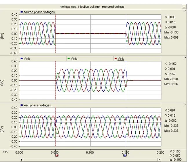
22 Fig. 7 and 8, respectively. Fig. 9 is a sample result for three-phase fault and restored voltage and Fig.10 is a sample result for three-phase fault with voltage harmonics compensation and restored voltage. The QPP is connected at 0.05 sec and off at 0.15 sec. Total simulation time with QPP is 0.1 sec and total simulation duration is 0.2 sec. QPP has restored the voltage at the sensitive load end to sinusoidal.

8. CONCLUSION

In this paper, the design of PLL with dqPLL technique, for improved performance of QPP in distorted supply condition is discussed.

The operation of the proposed scheme is verified by simulation using PSCAD and MATLAB / Simulink. The proposed system with dqPLL algorithm has superior performance and is able to operate in distorted supply conditions with high accuracy and has good dynamic time response. The simulation result shows the steady-state error is zero and the 2ω frequency oscillation error automatically goes to zero. Hence, this control approach achieves zero steady-state error voltage regulation. The proposed improvised technique is the most appropriate solution for the proposed control scheme for the QPP. The performance of the proposed dqPLL has been tested in all cases of voltage sags as well as with harmonics. The PI controller must be well tuned for optimum performance.

REFERENCES:

[1] Grady W.M, Samotyj M.J, Noyola A.H, “Minimizing Network Harmonic Voltage Distortion with an Active Power Line Conditioner”, IEEE Transaction on Power Delivery, pp. 1690-1697, Oct. 1991.

[2] Agileswari K.Ramasamy, Rengan Krishnan Iyer, Dr, Vigna K Ramachandaramuthy, Dr. R.N. Mukerjee, “Dynamic Voltage Restorer For Voltage Sag Compensation”, Power Electronics and Drives System, International Conference 28. Nov. 2005, Vol. 2, Pages 1289-1294.

[3] Timothy Thacker, “Phase locked loops using state variable feedback for single-phase converter systems”, IEEE, Applied Power Electronics Conference, pp. 864-870, 2009.

[4] H. Award, “Double Vector Control for series connected Voltage Source Inverter”, IEEE, Power Engineering Society, Vol.2, pp.707-712, 27-31 Jan. 2002.

[5] Adrian V. Timbus, “PLL Algorithm for Power Generation Systems Robust to Grid Voltage Faults”, IEEE, 37th Power Conference, pp.1-7, 18-22 June 2006.

[6] Sergio Franco, “Design with Operational Amplifiers and Analog Integrated Circuits”, 3rd Edition, Mc Graw-Hill, 2002.

AUTHOR PROFILES:

K. Chandrasekaran received the MSc degree in electrical and electronics engineering from University Technology PETRONAS in 2005. He is a PhD research scholar with the department of electrical and electronics engineering, UTP. His interest are power quality disturbances, FACT devices, active power filters and power systems.

Dr. K. S. Rama Rao received

23

24

T(sec) _{0.000 0.020 0.040 0.060 0.080 0.100 0.120 0.140 0.160 0.180} 0.0

1.0 2.0 3.0 4.0 5.0 6.0 7.0

P

L

L ang

le

in

(

rad

)

pll

ˆ θ

Fig. 5: Tracking of supply phase angle with dqPLL algorithm under distorted

and unbalanced condition in PSCAD

25

sec

P

L

L a

ng

le i

n

(

ra

d)

sec

P

L

L a

ng

le i

n

(

ra

d)

Fig. 7: Tracking of supply phase angle with dqPLL algorithm under distorted and unbalanced condition in SIMULINK

Time (sec)

P

LL an

gul

ar

f

re

q

ue

n

c

y

Time (sec)

P

LL an

gul

ar

f

re

q

ue

n

c

y

26

27