Data Processing Languages for Business Intelligence. SQL vs. R

Data Processing Languages for Business Intelligence. SQL vs. R

Marin FOTACHE

Al.I. Cuza University of Iasi, Romania fotache@uaic.ro

As data centric approach, Business Intelligence (BI) deals with the storage, integration, pro-cessing, exploration and analysis of information gathered from multiple sources in various for-mats and volumes. BI systems are generally synonymous to costly, complex platforms that re-quire vast organizational resources. But there is also an-other face of BI, that of a pool of data sources, applications, services developed at different times using different technologies. This is “democratic” BI or, in some cases, “fragmented”, “patched” (or “chaotic”) BI. Fragmenta-tion creates not only integraFragmenta-tion problems, but also supports BI agility as new modules can be quickly developed. Among various languages and tools that cover large extents of BI activities, SQL and R are instrumental for both BI platform developers and BI users. SQL and R address both monolithic and democratic BI. This paper compares essential data processing features of two languages, identifying similarities and differences among them and also their strengths and limits.

Keywords: Business Intelligence, Data Processing, SQL, R

Introduction

Often seen as a reincarnation of Decision Sup-port Systems [1] and sometimes referred as Business Intelligence and Analytics [2], Busi-ness intelligence (BI) is a broad category of

applications, technologies, and processes for gathering, storing, accessing, and analyzing data to help business users make better deci-sions [3]. Figure 1 displays a classical BI ar-chitecture [4].

Fig. 1. Typical BI architecture [4]

Common business intelligence related tasks are:

 data storage

 data extraction-transformation-load from various sources in a different for-mats, more or less structured, to the stor-age layer

 data processing

 information integration

 visualization

 exploratory analysis

 data mining/data science etc.

Analytics (BI&A) systems whore core tech-nologies have been:

 data management and warehousing [5] [6]

 text and web analytics for unstructured web contents [7]

 mobile technologies [8].

Implementation of BI platforms requires vast

quantity of organizational resources. Some of the most important current BI solutions are shown in figure 2 [9]. As with Enterprise Re-source Planning applications, BI systems im-plementation requires extensive organiza-tional changes and business expertise and sometimes it requires full vendor participa-tion.

Fig. 2. BI platforms [9]

Apart from impressive costs, BI platforms have the drawback of keeping captive the cus-tomer. Every organizational change and also new or updated external data source and ser-vice must be negotiated with BI platform pro-vider, which usually attracts new costs and also delays.

In this paper we scrutinize two languages, SQL and R, involved not only in BI applica-tion development but especially in the “de-mocratization” of BI as they allow various types of data professionals and users to access and process vast quantity of data in an inter-active, ad-hoc, way. Using two reliable sources, their role and popularity in current BI market will be outlined, taking into account job demand and a survey concerning BI tools and languages usage. Next the range of BI ac-tivities that can be supported by each SQL and R will be presented. The main section will compare SQL and R features syntax for the

most common data processing/reporting prob-lems, particularly important for BI users.

2 Languages and Tools for Business Intel-ligence

There is a vast array of tools, languages and technologies covering large extents of BI tasks. Some of them target regular users who are unable to write code and scripts in any pro-gramming language. Others are BI application

developer’s toolbox. But there some

technol-ogies that serve both users and developers in data processing, integration, visualization and analysis. Comparison of BI tools and lan-guages is also problematic because they can be available as programming languages, de-velopment environments, ecosystems or inte-grated platforms.

job trends. Figure 3 compares job demand in 2012-2016 interval for some of the most im-portant data processing and analysis lan-guages [10].

Fig. 3. Demand for main BI languages/tools [10]

SQL and R share most of the job postings. In 2012 SQL was by far the most demanded data language. Its share decreased slightly and seems to have stabilized since the end of 2014. R grew spectacularly in 2012-2014 interval, overpass SQL in 2014 for a brief period, and then fell back. Since 2014 it has fluctuated around 2% share. After SQL and R, the next popular is Python followed by SAS, SPSS, Stata and Julia. Currently there is still a visible lag between SQL-R group and the rest of the

languages/tools, although Python seems to in-crease steadily and might catch up with the leading group. SAS is not only a language, but also an integrated platform covering large sec-tions of BI applicasec-tions, whereas low figures for SPSS and Stata suggest they are used mainly in academia/research. Julia is a new-comer and it is unsure if it will reach the criti-cal mass adoption for being an important player.

The second source is annual KDnuggets Soft-ware Poll [11]. In the most recent edition, the 16th (2015), nearly 3000 voters choose from 93 different analytics and data mining tools. Results are displayed in figure 4. Survey re-vealed that R is the most popular overall tool among data miners, and Python is gathering traction steadily. RapidMiner continues to be most popular suite for data mining/data sci-ence. Hadoop/Big Data increased to 29%, up from 17% in 2014, and the fastest growth is for Spark whose usage share grew over 3-fold. KDnuggets Software Poll and indeed.com job trends confirm the centrality of both SQL and R as tools for BI users and developers.

3 SQL vs. R. The extent of analysis

As a data centric approach, BI heavily relies on various advanced data collection, extrac-tion, and analysis technologies, from Data Warehouse, extract – transform –load (ETL) tools, analytical processing (OLAP), ad-vanced reporting to adad-vanced knowledge dis-covery tools and techniques [2][12].

SQL and R languages are pivotal in BI data processing, as will be detailed in section 4. SQL and R are not only contenders, but also partners, especially when accessing and pro-cessing huge volumes of data stored in data-bases, data warehouses and Hadoop ecosys-tems. Feature comparison of table 1 is not in-tended to rank the first of two languages, but to outline the main areas SQL and R can be analyzed and compared, and also some areas where they do not really match, so the com-parison is fruitless.

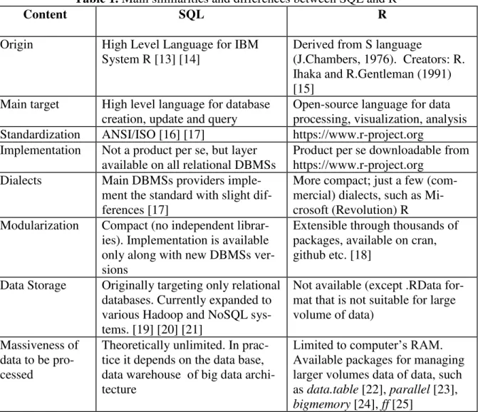
Table 1. Main similarities and differences between SQL and R

Content SQL R

Origin High Level Language for IBM System R [13] [14]

Derived from S language

(J.Chambers, 1976). Creators: R. Ihaka and R.Gentleman (1991) [15]

Main target High level language for database creation, update and query

Open-source language for data processing, visualization, analysis Standardization ANSI/ISO [16] [17] https://www.r-project.org

Implementation Not a product per se, but layer available on all relational DBMSs

Product per se downloadable from https://www.r-project.org

Dialects Main DBMSs providers imple-ment the standard with slight dif-ferences [17]

More compact; just a few (com-mercial) dialects, such as Mi-crosoft (Revolution) R Modularization Compact (no independent

librar-ies). Implementation is available only along with new DBMSs ver-sions

Extensible through thousands of packages, available on cran, github etc. [18]

Data Storage Originally targeting only relational databases. Currently expanded to various Hadoop and NoSQL sys-tems. [19] [20] [21]

Not available (except .RData for-mat that is not suitable for large volume of data)

Massiveness of data to be pro-cessed

Theoretically unlimited. In prac-tice it depends on the data base, data warehouse of big data archi-tecture

Limited to computer’s RAM.

Available packages for managing larger volumes data of data, such as data.table [22], parallel [23],

Data Sources Not related to the language, but dependent of DBMs. Usually lim-ited to databases created with a couple of SQL/relational DBMSs

Almost every data source (.csv, .xlsx, xml/html tables, relational databases, NoSQL data stores, Ha-doop etc.)

Table 1 (continued). Main similarities and differences between SQL and R

Content SQL R

Procedularity Implemented through section Per-sistent Stored Modules of the SQL standards; big differences among procedural extensions (PL/SQL, T-SQL, SQL PL, etc.) [17]

Native

Data Processing Best known language for pro-cessing data

Various features included in base R and especially a large number of packages.

SQL queries can be run with pack-age sqldf [26].

Two workhorses – packages dplyr

[27] and tidyr [28] OLAP Functions Implemented since SQL:2009

standard [16] [17] [29]

Implemented in dplyr package

Pivoting “Manual” [16], with recursive que-ries, or with pivot or model clauses [29] [30]

Package tidyr

Data Visualiza-tion

Simple (text-only) histograms [29] Excellent features and packages [31]: ggplot2 [32], lattice [33],

ggvis [34], googleVis [35] Data Analysis Initially only basic descriptive

sta-tistics [16]

Limited to some ANOVA, t-tests and basic non-parametric tests in some dialects (e.g. Oracle) [6]

Unlimited

Dynamics Mature.

Slow pace of implementing new features because of multitude of in-stitutions and companies involved in the standardization process

(Still) young.

Accelerate evolution, dozens of new packages every week.

Worries of becoming out of control

Learning curve Easy to learn Steep

Due to its processing power and accessibility, SQL has become the lingua franca of data pro-cessing. Its leading position seemed many times in jeopardy by the launch of languages like OQL and, more recently, NoSQL data stores and Hadoop systems [19]. But currently there is visible trend for adapting SQL even for NoSQL and Hadoop ecosystems [6] [19] [20]. That will reinforce SQL ubiquity since it

can process data stored on every data plat-form.

had been no match to the expressive power of SQL in terms of data processing options. Things are going to change, as seen in the next section. R is a vast endeavor. Data processed in R or within R but with SQL queries are ready to be explored, visualized, analyzed, and mined for patterns. In this respect, SQL cannot compete with R. Also R provides many other tools such as reporting (R Markdown), or even application development (Shiny) [36].

4 Main Data Processing Features in SQL

and R

The main area for a proper comparison be-tween SQL and R is data processing. This sec-tion will compare SQL and R features for some of the most frequent types of queries re-quired in BI. All the queries below were run on the database schema proposed by TPC-H benchmark [37], whose schema is depicted in figure 5. Tables were created in PostgreSQL and populated with random data using freely available dbgen tool [38].

Fig. 5. TPC-H benchmark database schema [37]

As in the current paper we did not test the per-formances of two systems, data were gener-ated just for scale factor of 0.1 with the fol-lowing number of records:

 5 in table REGION

 25 in table NATION

 15000 in table CUSTOMER

 1000 in table SUPPLIER

 20000 in table PART

 80000 in table PARTSUPP

 150000 in table ORDERS

 600572 in table LINEITEM

selected the shortest or the most readable. As SQL is a mature technology, we will provide some details just for the R queries.

Base R options are no match for SQL in terms or querying power. For displaying basic infor-mation about the quantity and prices of items sold within orders of January 1996 (second simple query in section 4.1), base R solution (with a little help from lubridate package) is:

library(lubridate) # package needed for functions "year" and "month"

t1 <- merge(orders, lineitem, by.x = "o_orderkey", by.y = "l_orderkey") t2 <- subset(t1, year(o_orderdate) == 1996 & month(o_orderdate) == 1,

select = c(o_orderkey, l_lin-enumber, l_partkey, l_quantity,

l_extendedprice, l_discount)) t2 <- transform(t2, line_amount = l_quantity * (l_extendedprice - l_dis-count))

t3 <- t2[order(t2$o_orderkey, t2$l_lin-enumber),]

The query is divided into a number of steps. The result of each step is a table that is pro-cessed by subsequent steps. The operating logic might be obvious, but the solution is cumbersome by any standard.

A series of packages, mainly dplyr and tidyr injected elegance and power into data pro-cessing in R. It is the main reason that on the subsequent examples, SQL syntax will be matched to syntax of (mainly) these two pack-ages).

4.1 Basic Queries (Selection, Projection, Join)

First simple query requires a few basic opera-tion: selection, projection, computed column, and sort - Display some basic information about the quantity and prices of items sold within orders 1284 and 1731. Below is the syntax for both SQL and R:

SQL: R (dplyr):

select l_or-derkey, l_lin-enumber, l_partkey, l_quantity, l_extend-edprice, l_dis-count, l_quantity *

(l_extend-edprice –

lineitem %>% filter(l_orderkey %in% c(1284, 1731)) %>% select (l_orderkey, l_linenumber, l_partkey, l_quan-tity, l_extend-edprice, l_discount) %>% mutate(line_amount = l_quantity * l_discount) as line_amount from lineitem where l_or-derkey in (1284, 1731) order by l_or-derkey, l_lin-enumber (l_extendedprice - l_discount)) %>% arrange(l_orderkey, l_linenumber)

The “pipe” operator (%>%) passes current op-eration result to the next opop-eration within the same query so there is no need to save inter-mediary results in separate data frames. Main predicate. Dplyr provides functions for each basic verb of data manipulation [27], from which in the query just

 filter() for selection of records

 arrange() for sorting records

 select() for (attributes) projection

 mutate() for adding computed columns.

The second simple query joins tables (data frames) orders and lineitem - Display basic in-formation about the quantity and prices of items sold within orders of January 1996:

SQL: R (lubridate and

dplyr): select o_or-derkey, o_order-date, l_linenumber, l_partkey, l_quantity l_extend-edprice, l_dis-count, l_quantity * (l_extendedprice – l_discount) as line_amount from orders in-ner join linei-tem

on o_orderkey = l_orderkey where extract (year from o_or-derdate)

= 1996 and ex-tract (month from

o_orderdate) = 1

order by o_or-derkey, l_lin-enumber

library(lubridate) orders %>%

inner_join(lineitem, by = c('o_orderkey'= 'l_orderkey' )) %>%

filter(year(o_order-date) == 1996 & month(o_orderdate) == 1) %>%

Syntax for the inner join is close enough to that of SQL. Similarly dplyr implements outer joins and semi joins, but also the anti-join, which is not available in too many SQL dia-lects.

4.2 Aggregate Queries

Similar to SQL, dplyr offers group_by() func-tion. It breaks down a dataset into specified groups of rows so that when applying a verb to the resulting object, the verb will be per-formed for each group. Grouping affects the verbs as follows:

 grouping variables are always retained in the result

 grouped arrange() orders first by the grouping variables (which is not the case in SQL)

mutate() and filter() are most useful in conjunction with window functions

 slice() extracts rows within each group.

 summarise() allows defining aggre-gate variables

First problem requiring basic aggregation with group filter is Display monthly sales for years 1996-2000 that are greater than one bil-lion:

SQL: R (lubridate and

dplyr):

select extract (year from o_or-derdate)

as year, ex-tract (month from

o_orderdate) as month, sum( l_quan-tity *

(l_ex-tendedprice –

l_discount)) as monthly_sales from orders in-ner join linei-tem

on o_orderkey = l_orderkey where extract (year from o_or-derdate)

between 1996 and 2000 group by year, month

orders %>%

inner_join(lineitem, by = c('o_orderkey' = 'l_orderkey' )) %>%

filter(year(o_order-date) >= 1996 & year(o_orderdate) <= 2000) %>%

group_by(year = year(o_orderdate), cmonth =cmonth(o_order-date)) %>% summa-rise(monthly_sales = sum(l_quantity *(l_extendedprice - l_discount)) ) %>% filter (monthly_sales > 1000000000) %>% arrange(year, month) having sum( l_quantity * (l_extend-edprice - l_dis-count)) > 1000000000 order by year, month

Here there is a slight advantage of dplyr due to the pipe operation, so that the expression for group filtering does not have to define repeat-edly the expression for aggregation.

Second aggregate queries answers a problem with subtotals - Display monthly sales for years 1996-2000 with subtotals on each year:

SQL: R (lubridate and

dplyr):

select extract (year from o_or-derdate) as year, extract (month from o_orderdate) as month, sum( l_quantity * (l_extend-edprice - l_dis-count)) as

monthly_sales from orders in-ner join linei-tem on

o_orderkey = l_orderkey where extract (year from o_or-derdate) between 1996 and 2000

group by year, month

union select extract (year from o_or-derdate) as year, null as month, sum( l_quantity * (l_extend-edprice - l_dis-count)) from orders in-ner join linei-tem

on o_orderkey = l_orderkey where extract (year from o_or-derdate) between 1996 and 2000 bind_rows (orders %>% inner_join(linei-tem, by =

c('o_orderkey' = 'l_orderkey' )) %>% filter(year(o_or-derdate) >= 1996 & year(o_orderdate) <= 2000) %>%

group_by(year = year(o_orderdate), month = month(o_orderdate)) %>% summa-rise(monthly_sales = sum(l_quantity *

(l_extendedprice –

l_discount)) ),

orders %>%

inner_join(linei-tem, by c(

'o_orderkey' = 'l_orderkey' )) %>% filter(year(o_or-derdate) >= 1996 & year(o_order-date) <= 2000) %>% group_by(year = year(o_orderdate), month = NA) %>%

summa-rise(monthly_sales = sum(

l_quantity *

(l_extendedprice –

l_discount)) ) ) %>%

group by year order by year, month

Pipe operator was no useful in this case, so SQL query is shorter. Function bind_rows() in dplyr is the equivalent of UNION SQL opera-tor.

4.3 Subqueries

There are numerous problems to be answered using what is SQL are called as subqueries. In SQL queries can be part of WHERE, HAV-ING, FROM, SELECT and WITH clauses. In dplyr there are no such differences.

First problem answered in SQL with a subquery placed into WHERE clause is Re-trieve orders issues in the same day as the or-der 3271:

SQL: R (lubridate and

dplyr): select o_orderkey, o_custkey, o_orderstatus, o_orderdate, o_orderpriority from orders where o_orderdate in (select o_orderdate from or-ders where o_orderkey = 3271)

orders %>% filter (o_order-date %in% ( orders %>% fil-ter (o_orderkey == 3271)) [['o_orderdate']]) %>% select (o_or- derkey:o_order-priority)

Here required attributes were consecutive. That shortened the projection clause (select) in the dplyr query. Also notice %in% opera-tor, which is the counterpart of SQL IN. The second problem for illustrating subqueries implies group filtering is Extract day (or days, if there are more than one) with the maximum number of orders. Three SQL solutions and two dplyr “counterparts” will be provided as follows:

SQL – solution based on a subquery in

HAVING clause:

R (lubridate and dplyr):

select o_order-date, count(*) as n_of_orders from orders orders %>% group_by(o_order-date) %>%

group by o_order-date

having count(*) = (select count(*) as n_of_orders from orders group by o_orderdate order by n_of_orders desc limit 1) summa-rize(n_of_orders = n()) %>% filter (n_of_orders >= max(n_of_orders))

SQL – solution based on a subquery in

FROM clause

R (lubridate and dplyr): select dates_n_of_or-ders.* from (select o_order-date, count(*) as n_of_orders from orders group by o_or-derdate) dates_n_of_orders inner join (select count(*) as n_of_orders from orders group by o_or-derdate order by n_of_orders desc limit 1) max_n_of_orders on dates_n_of_or-ders.n_of_orders = max_n_of_or-ders.n_of_orders orders %>% group_by(o_order-date) %>% summarize(n_of_or-ders = n()) %>% inner_join( orders %>% group_by(o_or-derdate) %>% summa-rize(n_of_orders = n()) %>% arrange (desc(n_of_orders) ) %>% top_n(1))

SQL – solution based on table ex-presssion

R (lubridate and dplyr) – repeated:

Now dplyr syntax looks more powerful and elegant. Second dplyr solution contains an OLAP (window) function – top_n().

The third problem involves group comparison - Extract dates with at least the number of or-ders issued on 1993-04-21:

SQL – solution based on table ex-presssion R (dplyr): with dates_n_of_orders as (select o_order-date, count(*) as n_of_or-ders

from orders group by o_or-derdate) select * from dates_n_of_orders where n_of_orders >= (select n_of_orders from dates_n_of_orders where o_or-derdate = DATE'1993-04-21') orders %>% group_by(o_order-date) %>% summarize(n_of_or-ders1 = n()) %>% mutate(

n_of_orders2 = ifelse(o_or-derdate == '1993-04-21',

n_of_or-ders1, 0), n_of_orders3 = sum(n_of_orders2) ) %>% filter (ders1 >= n_of_or-ders3)

Here a dplyr trick was needed in order the groups to be compared. After computing the number of orders for each date (n_of_or-ders1), we create a variable (n_of_orders2), which is zero for all of the dates except the date of reference (1993-04-21). Only for this date n_of_orders2 has the same value as n_of_orders1. The third new variable (n_of_orders3) stores the number of orders for the reference date and it was used for filtering the groups.

4.4 Pivoting

Pivot tables is one the key features in BI re-porting and analysis. Many relational/SQL DMBSs have implemented PIVOT clause for answering this type of problems [29] [30]. Un-fortunately, currently PostgreSQL does not support dynamic pivoting. Function CROSS-TAB requires explicit definition of all column of the pivoting operation. This is acceptable from small number of columns and awkward

for the rest of the cases. Consequently, for the problem Display product sales for sales years between 1991 and 2000 only dplyr solution will be presented:

orders %>%

inner_join(lineitem, by = c('o_orderkey' = 'l_orderkey' )) %>%

filter(year(o_orderdate) >= 1991 &

year(o_orderdate) <= 2000) %>%

inner_join(part, by = c('l_partkey' = 'p_partkey' )) %>%

group_by(products = p_name, year =

year(o_orderdate)) %>%

summarise(sales = sum(l_quantity * (l_extendedprice - l_discount))) %>% spread (year, sales, fill=0)

4.5 Recursivity

Introduced by ANSI SQL:1999 standard and implemented almost all major relational DBMSs, recursive queries (WITH RECUR-SIVE) are extremely powerful tools for data-base processing and remains largely un-derused by database professional. Recursivity is needed, for example, when the number of levels in tree (hierarchical structure) varies from one organization to another and there is a need to display, for each employee, the en-tire managerial path (from she/he until the top manager).

TPC-H schema does not contain a proper hi-erarchical structure. Nevertheless, the are types of problems that require recursivity. For example, Display, for each product, a string with the list of first 5 customers (in alphabetic order) that have purchased it:

SQL – solution based on recursive query built with a table ex-presssion

R (dplyr and tidyr):

with recursive prod__cus-tomer_list (p_name, p_part-key, cust_no, cust_list) as ( select pc.p_name, pc.p_partkey, pc.cust_no, cast (pc.c_name as var-char(100000) ) from pc part %>% inner_join(lin-eitem, by = c('p_partkey' = 'l_partkey')) %>%

inner_join(or-ders, by = c( 'l_orderkey' = 'o_orderkey')) %>%

where cust_no = 1

union all

select pc.p_name, pc.p_partkey, prod__cus-tomer_list.cust_no + 1,

cast

(prod__cus-tomer_list.cust_li st ||

', ' || pc.c_name AS var-char(100000) ) from pc inner join prod__cus-tomer_list

on pc.cust_no =

prod__cus-tomer_list.cust_no

+ 1 ),

pc as (select * from ( se-lect p_name, p_partkey, c_name, row_num-ber() over (partition by p_name

or-der by c_name) as cust_no

from

part inner join lineitem on p_partkey = l_partkey

inner join orders on

l_orderkey =

o_orderkey

inner

join customer on o_custkey = c_cus-tkey) x

where cust_no <= 5)

select p_name, cust_list from prod__cus-tomer_list order by p_name

select (p_name, c_name) %>% group_by(p_name) %>%

slice(1:5) %>% group_by(p_name)

%>%

summa-rise(five_cust_li st =

paste(c_name,

collapse=", "))

From this example one might conclude that dplyr syntax is considerable more elegant in solving problems requiring recursive queries.

4.6 OLAP functions

In SQL OLAP functions, labeled also as ana-lytic or window functions were added in SQL:1999 standard. In R dplyr provides a large number of window functions such as:

 lead - to copy with values shifted by 1

 lag - to copy with values lagged by 1

 dense_rank - to rank with no gaps

 min_rank – ranks; ties get min rank

 percent_rank - ranks rescaled to [0, 1]

 row_number - ranks; ties got to first value

 ntile - bin vector into n buckets

 cume_dist - cumulative distribution

 cumall - cumulative all.

An example of such analytic function was in-cluded in a previous query. Because the logic of these functions is quite similar to their SQL counterparts, no additional example will be provided.

5 Conclusions

For Business Intelligence SQL and R are core technologies. Addressing all the range of pro-fessionals between BI application developers and qualified users, both languages support BI decentralization, modularization, flexibility and, ultimately, the BI democratization. SQL is the real Esperanto of the data pro-cessing languages. Since now, all the chal-lengers (OQL, NoSQL and some Hadoop sys-tems) ended in adopting a more SQL look or face extinction.

Various information sources show that both SQL and R have leading positions in profes-sional BI profesprofes-sionals and job market de-mand.

Covering different segments of BI activities, both languages share data processing and re-porting segment. This paper argues that, with new packages like dplyr and tidyr, R can com-pete with SQL in terms of processing power and syntax elegance.

References

for Information Systems, vol. 13, Special Issue, pp. 315-340, May 2012

[2] H. Chen, R.H.L. Chiang, and V.C. Storey,

“Business Intelligence and Analytics: From Big Data to Big Impact,” MIS Quar-terly, vol. 36, no. 4, pp. 1165-1188, De-cember 2012

[3] H.J. Watson (2009). Tutorial: Business In-telligence – Past, Present, and Future,"

Communications of the Association for In-formation Systems [Online]. Vol. 25, Ar-ticle 39. Available: http://ai-sel.aisnet.org/cais/vol25/iss1/39

[4] S. Chaudhuri, U. Dayal, and V. Narasayya,

“An overview of business intelligence technology,“ Communications of the ACM, vol. 54, no. 8, pp. 88-98 (August 2011)

[5] C. Strimbei. (2012). OLAP Services on Cloud Architecture. Journal of Software & Systems Development [Online]. 2012, Ar-ticle ID 840273. Available: http://www.ibimapublishing.com/jour-nals/JSSD/2012/840273/840273.pdf

[6] M. Fotache and C. Strîmbei, “SQL and Data Analysis. Some Implications for Data Analysts and Higher Education,” in

Proc. of the Globalization and Higher Ed-ucation in Economics and Business Ad-ministration (GEBA 2013), Al.I.Cuza University, Iasi, 2013, published in Proce-dia Economics and Finance, 20 (2015), pp. 243 – 251.

[7] G. Zheng and S. Peltsverger. Web Analyt-ics Overview in Encyclopedia of Infor-mation Science and Technology, Third Edition, Chapter: 756, IGI Global, 2014. Available: https://www.re-

searchgate.net/publica- tion/272815693_Web_Analytics_Over-view

[8] O. Dospinescu and M. Perca. (2013). Web Services in Mobile Applications.

Infor-matica Economică Journal [Online]. 17(2), pp.17-26. Available: http://re-

vistaie.ase.ro/content/66/02%20-%20Dospinescu,%20Perca.pdf

[9] B. Evelson (2015, September 25). The Forrester Wave: Agile Business Intelli-gence Platforms, Q3 2015. Available:

http://go.sap.com/docs/download/2015/09

/541ccd61-437c-0010-82c7-eda71af511fa.pdf

[10] *** (2016, April 30). Python, SQL, R, SPSS, SAS, Stata, Julia Job Trends. Avai-lable: http://www.indeed.com/job- trends/q-Python-q-SQL-q-R-q-SPSS-q-SAS-q-Stata-q-Julia.html

[11] *** (2015, December 20). Analytics, Data Mining, Data Science software/tools used in the past 12 months. Available: http://www.kdnuggets.com/polls/2015/an alytics-data-mining-data-science-soft-ware-used.html

[12] E.P. Lim, H. Chen, G. Chen, "Business Intelligence and Analytics: Research Di-rections," ACM Transactions on Manage-ment Information Systems, Vol. 3, No. 4, Article 17, January 2013.

[13] D. Chamberlin, R.F. Boyce (1974). SE-QUEL. A Structured English Query Lan-guage. Available: http://www.alma- den.ibm.com/cs/people/chamberlin/se-quel-1974.pdf

[14] D.D. Chamberlin, M.M. Astrahan, M.W. Blasgen, J.N. Gray, W.F. King, B.G. Lind-say, R. Lorie, J.W. Mehl, T.G. Price, F. Putzolu, P. Griffiths Selinger, M. Schkol-nick, D.R. Slutz, I.L. Traiger, B.W. Wade, and R.A. Yost, “A history and evaluation

of System R,” Communications of the ACM, vol. 24, no.10 , pp.632-646, October 1981

[15] R. Ihaka, R. Gentleman, "R: A Language for Data Analysis and Graphics," Journal of Computational and Graphical Statis-tics, vol. 5, no. 3, pp.299–314, 1996 [16] J. Celko, SQL for Smarties. Advanced

SQL Programming (3rd edition). San Fran-cisco: Morgan Kaufmann, 2005

[17] A. Kriegel and B.M. Trukhnov, SQL Bi-ble (2nd edition). Indianapolis: Wiley, 2008 [18] A. Decan, T. Mens, M. Claes, and P. Grosjean, “On the Development and Dis-tribution of R Packages: An Empirical Analysis of the R Ecosystem,” in Proceed-ings of the 2015 European Conference on

Software Architecture Workshops

[19] I. Hrubaru and M. Fotache, “On a Ha-doop Cliché: Physical and Logical Models Separation,” in Proc. of the 14th Interna-tional Conference on Informatics in Econ-omy (IE 2015), Bucharest, Romania, 2015, pp. 357-363

[20] M. Armbrust, R. S. Xin, C. Lian, Y. Huai, D. Liu, J. K. Bradley, X. Meng, T. Kaftan, M.J. Franklin, A. Ghodsi, and M. Zaharia,

“Spark SQL: Relational Data Processing

in Spark,“ in Proc. of the 2015 ACM SIG-MOD International Conference on Man-agement of Data (SIGMOD '15). Mel-bourne, Victoria, Australia, pp. 1383-1394.

[21] Y.N. Silva, I. Almeida, and M. Queiroz,

“SQL: From Traditional Databases to Big Data,” in Proc. of the 47th ACM Technical Symposium on Computing Science Educa-tion (SIGCSE '16). Memphis, Tennessee, USA, pp. 413-418.

[22] M. Dowle, A. Srinivasan, T. Short, S. Li-anoglou, R. Saporta and E. Antonyan (2015). data.table: Extension of Data.frame. R package version 1.9.6. Available: https://CRAN.R-pro-ject.org/package=data.table

[23] R Core Team (2016). R: A language and environment for statistical computing. R Foundation for Statistical Computing, Vi-enna, Austria. Available: https://www.R-project.org/

[24] M.J. Kane, J. Emerson, and S. Weston,

“Scalable Strategies for Computing with Massive Data,” Journal of Statistical Soft-ware, vol. 55 no. 14, pp.1-19, 2013. [25] D. Adler, C. Gläser, O. Nenadic, J.

Oehlschlägel and W. Zucchini (2014). ff:memory-efficient storage of large data on disk and fast access functions. R pack-age version 2.2-13. Available: https://CRAN.R-project.org/package=ff [26] G. Grothendieck (2014). sqldf: Perform

SQL Selects on R Data Frames. R package version 0.4-10. Available:

https://CRAN.R-project.org/pack-age=sqldf

[27] H. Wickham and R. Francois (2015). dplyr: A Grammar of Data Manipulation. R package version 0.4.3. Available:

https://CRAN.R-project.org/pack-age=dplyr

[28] H. Wickham (2016). tidyr: Easily Tidy Data with `spread()` and `gather()` Func-tions. R package version 0.4.1. Available:

https://CRAN.R-project.org/pack-age=tidyr

[29] A. Molinaro, SQL Cookbook. Sebastopol

(CA): O’Reilly, 2006

[30] S. Faroult, The Art of SQL. Sebastopol (CA): O’Reilly, 2006

[31] W. Cho, Y. Lim, H. Lee, M. K. Varma, M. Lee, and E. Choi, “Big Data Analysis with Interactive Visualization using R packages,“ in Proc. of the 2014 Interna-tional Conference on Big Data Science and Computing (BigDataScience '14), Beijing, China, 2014, Article 18, 6 pages [32] H. Wickham, ggplot2: Elegant Graphics

for Data Analysis. New York: Springer-Verlag, 2009.

[33] Sarkar, Deepayan, Lattice: Multivariate Data Visualization with R. New York: Springer Verlag, 2009

[34] W. Chang and H. Wickham (2015). ggvis: Interactive Grammar of Graphics. R package version 0.4.2. Available:

https://CRAN.R-project.org/pack-age=ggvis

[35] M. Gesmann and D. de Castillo, “Using

the Google Visualisation API with R,” The R Journal, vol 3, no. 2, pp. 40-44, Decem-ber 2011.

[36] A. Cirillo, RStudio for R Statistical Com-puting Cookbook, Birmingham, UK: Packt Publishing, 2016

[37] TPC BENCHMARK H (Decision Sup-port) Standard Specification Revision

2.17.1, 2014, Available:

http://www.tpc.org/tpc_documents_cur-rent_versions/pdf/tpc-h_v2.17.1.pdf [38] T. Kejser (2014).Tpch-dbgen Overview,

Internet:

https://bit-bucket.org/tkejser/tpch-dbgen