Product Design and Process Planning in Using the Process Capability Index

! "

# "

" # ! $ "

! $

# ! % "

&

" !

' " "

!

"

! $

! $

! $

!

"

!

(

) !

I. INTRODUCTION

Today's manufacturing industry is facing intensive competition, so both the cost and quality aspects have become important issues among management concerns. Thus producers thrive on providing economical processes which are also capable of meeting the customer's quality requirement. In recent years, as the concept of concurrent engineering has become widely accepted, design engineers hope to achieve simultaneous product design and process planning, side by side, at an early stage of product development [4]. The goals are to shorten the time span required for introducing the new product onto the market and to attain the lowest production cost and premium product quality. Hence, what is needed is a way to measure the degree of the producer's process capability, in satisfying the customer's quality requirement. More importantly,

Manuscript received December 9, 2008. This work was carried out in the Design, Quality, and Productivity Laboratory (DQPL) at the Department of Industrial Engineering and Systems Management at Feng Chia University, Taichung, Taiwan under Grant no. 97822218E80358058 from the National Science Council of the Republic of China.

Angus Jeang is with the Department of Industrial Engineering and Systems Management, Feng Chia University, Taichung, Taiwan, R.O.C. (e8mail: akjeang@fcu.edu.tw).

Chien8Ping Chung is with the Department of Industrial Engineering and Systems Management, Feng Chia University, Taichung, Taiwan, R.O.C. (corresponding author to provide phone: +88684824517250; fax: +88684824510240; e8mail: p9317369@ fcu.edu.tw).

a growing number of producers include this measurement value in their purchase contracts with customers, as a documentation requirement. One such measurement is the process capability index (PCI).

The process capability index (PCI) is a value which reflects real8time quality status. The PCI acts as the reference for real8time monitoring that enables process controllers to acquire a better grasp of the quality of the_mon site processes [6,7]. Although the PCI is considered as one of the quality measurements employed during on8line quality management, several authors have pointed out that the PCI should be addressed at the beginning of the design stage rather than at the production stage, where process capability analysis is typically done [12]. For the sake of convenience, let us call the PCI for the former one, off8line PCI, and the latter one, on8line PCI. The on8line PCI has process mean and process variance that are obtained from the existing process. Conversely, the off8line PCI has the process mean and process variance as two unknown variables, which the process planner would have to determine. When cost is not considered as a factor for off8line PCI analysis; normally the process planners would do their best to set the process mean close to the design target, and minimize the process variance. Because the additional cost incurred for tightening the variance is not considered, obviously, the establishment of mean and variance values will result in a high PCI scale [9]. Thus, this research intends to develop an Off8line PCI that expression which contains cost factors.

The PCI value is typically defined as the ability to carry out a task or achieve a goal. In process capability analysis, the lower and upper limits are initially assumed to be firm and non8negotiable, unless it can be proven that the quality of the final product will not be lessened by changing these limits. The controllable factors are the process mean and process variance [8]. The deviation between process mean and design target can be reduced by locating the process mean close to the design target without additional cost being incurred. The process variance can be lowered by tightening the process tolerance, with extra cost incurred. In case the conventional on8line PCI is used for process capability analysis during the product development, designer engineers naturally intend to raise the PCI value by locating the process mean near the target value, and by reducing the tolerance value to ensure a better product quality. However, simply increasing the PCI value can easily create additional and unnecessary production costs that result from extra efforts and expensive devices for ensuring tolerance control. Hence, there is a need to balance customer demands for quality and production costs. In this regard, the off8line PCI value is introduced, in consideration of quality loss and production cost, simultaneously in this research. The quality loss is expressed by quality loss function, and the production cost is represented by tolerance cost function. Then, this new PCI expression can be used as linkage for concurrent product design and process planning, prior to actual production. The

*

+

-II. BACKGROUND REVIEW

The process design requires determining the best quality value of process setting and process tolerance so that unit8to8unit variation is reduced to a minimum. Process tolerance is defined as the maximum range of variation for the quality value of interest in a particular process. By following the selected process setting and process tolerance, the quality value of production output is randomly distributed, with the average and variability being process mean and process variance. To reduce the variation of production output so that the functionality of a produced product can be accomplished, we usually have a process specification as maximum value of production output, which allows for deviation from the target value.

The process mean may or may not be same as the quality value of the process setting. By the same token, the process variance may or may not be the same as the quality value established by the process tolerance. However, having the process setting and process tolerance established at process design, with the possibility of process drifting or systematic error being excluded in the production process, we believe that the process mean will be close to the selected process setting, and that the process variance will be less than the process tolerance after production process. Suppose that X1, X2, …, Xn

are the produced quality values. The sample average is:

1

=

∑

(1)

The sample standard deviation is: 1

2

2

1

(

)

[

]

=

−

∑

(2)

The parameter is the established process setting (process mean), and parameter

σ

is the process standard deviation estimated from determined process tolerance Obviously, and

σ

are population mean and population standard deviation of the produced quality values. Thus, assume that the probability distribution of population representing the produced quality values, forms a normal distribution with X ~ N( ,

σ

2) from which the sample was taken. Both the mean and tolerance are two controllable variables which can be decided at the very beginning of the process or product design, namely, pre8production stage. It is believed that and observed from the samples will be close to and

σ

as the sample size becomes great. For the sake of convenience, we will call these two statistics the process mean and process tolerance, in the following discussion.

In the product life cycle, quality values will vary under different circumstances. Fig. 1 is a typical quality loss function. Let X1,X2,…, Xnbe the quality values appearing in

different situations. The average quality loss in its symmetric quality loss function is the following [11,14]:

E[L(X)] =

[(

−

)

2

+

σ

2

]

(3)

U represents the average value of the quality characteristic, while σ2is the variance of the quality characteristic. Equation (3) tells us that there are two sources of quality loss. (a) K(U–T)2is the deviation between the process mean and the design target. Examples are blade damage, machine breakdown, problems with raw materials and worker carelessness, which are usually easy to handle without cost becoming a factor. (b) Kσ2is the loss resulting from process variances. To eliminate this source, better equipment, materials, and processes are usually required. There is cost containment in this effort. Hence, we usually improve (a) first, and then (b), for economic considerations.

Usually, a high tolerance cost is associated with a tight process tolerance, while a low tolerance cost results from a loose process tolerance. Fig. 2 is a typical tolerance cost function. The tolerance cost can be formulated in various function expressions. To evaluate the tolerance cost, this paper adopts the tolerance cost function as developed in the literature [3].

CM(t) = a＋b．exp (–c．t ) (4)

where a, b, and c are the coefficients for the tolerance cost function, and t is the process tolerance. From the above cost expression, it can be noted that a tight process tolerance results in a higher tolerance cost, due to additional manufacturing operations, more expensive equipment needed and slower production rates, while a loose process tolerance results in a lower tolerance cost [8810].

T8S T T+S

L(X)

0

X

Fig. 1. Quality loss function

t

CM(t)

0

! " !#

The frequently seen PCI includes Cp, Cpk, and Cpm

expressions. Cpcan be defined as follows [1,2,5,6,7].:

σ $

% % &

% ₍₅₎

The expression (USL8LSL) refers to the difference between the upper and lower limits which are specified by the customer's quality requirement;

σ

is the standard deviation which is actually incurred in the production process. However, during the production process, the process means U can be located at positions other than design target. If the process variance

σ

2 did not change, the above Cp value would also remain

unchanged; this was the major defect owing to the facts that only the spread of the process is reflected, and the deviation of process mean can not be reflected in the measurement. These are the main reasons why Cpkwas developed; the Cpkexpression

is defined as below:

) 3 , 3 (

σ σ

% % & &

% '

( (6)

There is still a deficiency for Cpk expression: the same Cpk

values may be constituted with different process means and variances. This situation has created a great deal of confusion, and uncertainty as to which would be the best process capability among the alternatives. To cope with the above arguments, another form of PCI, Cpm, was developed. Cpm is defined as

follows:

# & " ) $

% % & %

* *

σ

(7)

When the process mean is equal to design target, the Cpmcan be

simplified as Cp. For the purpose of comparison, three

processes: A, B, and C are depicted in Fig. 3. The Cp, Cpk, and

Cpmvalues from processes A, B, and C are shown in Table 1.

Because process C has the greatest Cpvalue, it is might be

mistakenly concluded that process C had the best process capability among processes A, B, and C, when Cpis considered

as a reference value. However, this erroneous conclusion originates from the fact that the Cpvalue is solely based on the

magnitude of variance, and disregards the negative impact from the process deviation. Similarly, when Cpk was used in

representing the levels of process capability, the process Cpk

values for processes A, B, and C, are all just equal to one. Thus again, quite obviously, there is difficulty in ordering the superiority of process capability of the three processes. To overcome the defects appearing in Cp and Cpk expressions,

another PCI expression, Cpm,is introduced. Unlike the previous

two expressions, Cpm can simultaneously reflect the impact

from process deviation and process variance. This feature is particularly important because process mean and process variance are generally changed at the same time in most production process. Unfortunately, with Cpm, processes A and

B are the best two choices. The non8different outcomes between processes A and B result from the fact that the contribution of Cpm value, from process mean deviation and

process variance magnitude, is identical. Hence, there must be a way of measurement being provided to make mean deviation and process variance magnitude distinguishable in PCI expression.

Fig. 3. The distribution for process A, B and C

Note: Process A: UA= 50.0,

σ

=5.00, CM(t)=$2000,

Process B: UB= 53.0,

σ

=3.83, CM(t)=$3500,

Process C: UC= 57.5,

σ

=2.50, CM(t)=$6000

Table 1 PCI values for process A, B, and C

Process Cp Cpk Cpm Cpmc

A 1 1 1 0.051298

B 1.25 1 1 0.047673

C 2 1 0.632456 0.031782

+ ,

-An assembled product consists of several components created by different processes; hence, determining which combination of component tolerances is best, is an important issue. In addition to tolerance design for a single component of a product, most design problems should allocate component tolerances so that the assembly dimensions of a completed product fall into acceptable quality and functionality limits. The assembly dimension of a completed product is a combination of the dimensions of several components from assembly chains; therefore, the overall assembly dimensions vary within a distributed range. As a result, most tolerance analyses with assembly dimensions relate the variation of assembly tolerances (resultant tolerances) to the variation of the component tolerances, whereby appropriate component tolerances are determined.

Thus, to extend tolerance design for a completed dimension, tolerance stack8up and variance build8up models will be applied. Tolerance stack8up and variance build8up are estimated by using the assembly chain, where the formation of tolerance stack8up is accumulated by the product/process tolerances appearing in the related components in the assembly chain. Similarly, the variance build8up possesses the same features, that is, worse cases of tolerance stack8up and variance build8up can be represented as:

0

1

'

.=

≈

_∑

Y j

t

t

(8)

0

1

'

.=

≈

∑

2 2

Y j

σ

σ

(9)

where tjis the process tolerance of the jthcomponent/process,

Y

total number of the components in a product. The term

σ

2_j is the process variance of the jthcomponent/process, which can also be estimated as: ₍ tj ₎2

P

, where P is a given value [10], while

σ

_Y2 is the process variance build8up of the product quality value (also called resultant process variance).

Let XYrepresent the resultant product quality value that is

summed up from several single component product quality values:

0

1

'

. . / .=

× =

∑

(10)

Ajis the assembly chain vector for the jthcomponent. The

example in this study discusses an assembly chain vector that involves linear equations with coefficients being 1 or 81; Xjis

the single product quality value. By taking the expectation on both sides of (10), the expected value of the resultant product quality value is:

0

1

'

. . / .=

× =

∑

(11)

Ujis the process mean of a single product quality value and

UYis the resultant process mean.

III. SIMULTANEOUS DETERMINATION OF PARAMETER AND TOLERANCE VALUES

Product functionality is achieved through the assignment of appropriate design target and design tolerance, at the stage of product design and process planning. Generally, when the manufacturer attempts to attain a high process capability with a small process tolerance, a higher manufacturing cost will usually result. But when the design tolerance exceeds the process tolerance, additional space or process distribution is provided for a possible shift or drift. Consequently, the parameter value may be set at various positions within a feasible range, which in turn, can lead to quality improvement and cost reduction. The mathematical relationship of the design target , design tolerance , parameter value and process tolerance , can be represented as [8]:

∣ 0 ∣∣ 0 (12)

The tolerance value is constrained by %and which refer to

upper and lower process capability limits, respectively. However, the parameter value is also contained within an acceptable range, between and %. That is,

%

≤ ≤

(13)

%

≤ ≤

(14)

The values of %, , , %, , and are known in advance.

Equation (12) states that the deviation between design target and parameter value should be less than the distance between design tolerance and process tolerance. By satisfying (12), manufacturability for all possible combinations will be ensured. As a result, the feasible combinations increase the flexibility of both product design and process planning, to a great amount. In addition, the effort of obtaining the precision required for the control of the process is reduced. Quality improvement and cost reduction are thus achieved. In general, there are no costs associated with the parameter design which changes the nominal value of a parameter value; conversely, there are costs involved in the tolerance design. Hence, the best setting of the nominal values is often determined prior to the tolerance design,

for the sake of economics. However, based on the discussion regarding (12), in some situations it is important to simultaneously determine parameter and tolerance values, due to the dependency between these two values on the quality characteristics of interest. The dependency phenomena discussed in (12) mainly focus on one single quality characteristic. However, the dependency phenomena are still true in a design with multiple quality characteristics. This is due to the fact that (20) and (23) or (26) and (29), shown in Appendix, are mutually dependent when design function "1#is a nonlinear function. The mutual dependency can be explained by the fact that /and /are in a functional relationship with

component parameter value , and tolerance value concurrently. Because /and /still need to be constrained by

(12), and will be substituted into the PCI expression eventually, the degree of dependency will be even greater than in the former situation. Although, most of the time design function "1# is unknown, we believe that it should inherently exist in a nonlinear function form, for all product design and process planning. Based on the above discussion, both the parameter and tolerance values have to be simultaneously determined in order to optimize the design.

IV. PROCESS CAPABILITY INDEX FOR OFF8LINE APPLICATION

2

-The conventional PCI values are mainly applied to measure the on8line spread resulting from actual process deviation and process variance. The reality of this spread is a consequence of the production process, in which there are no more controllable elements. Hence, the conventional PCI expression is valid only in the on8line application. In this regard, there is an attempt to explore the process capability analysis, at the pre8production stage, to enable designers to integrate the aspects of product design and process planning at an early time. According to the preceding discussion, unlike the other two PCI expressions, Cpm

is able to simultaneously reflect the influences of process deviation and process variance. However, this is only legitimate at the post8production stage, due to the fact that U and t are realized values which are not controllable for design. However, when Cpmis used as a measurement scale in the pre8production

stage, U and t become controllable variables. Then, it is possible that various combinations of U and t will result in the same Cpmvalue. Thus, it is difficult to make a distinction among

alternatives, in order to make a correct choice from among them. As is known, the process mean U can be adjusted at no additional cost. The designers would most likely establish the process mean U as close as possible to the design target T, within the process feasible range, and attempt to decrease the process variance as much as possible within the process capability limits in order to attain a higher PCI value. In other words, with the exclusive use of the process mean and process tolerance as the determinants of conventional PCI, regardless of the cost impact on customer and production, there is a tendency for designers to position the process mean as close to the target value as possible, and solely cut down the process tolerance to lower capability limit in order to increase the PCI value. Apparently, the found PCI value is erroneous.

value through tolerance design which usually involves additional cost. Therefore, in addition to the constraints from feasible ranges and capability limits, the influence exerted by the relevant costs representing the selected process mean and process tolerance, should be considered as well. This brings us to the next section, a discussion on the requirement that costs related to process mean and process tolerance must be contained in PCI expression, when referred to as off8line process capability analysis, during product design and process planning.

As indicated in Fig. 4, various combinations of U and t will result in the same Cpmvalue, 1.2. This unhelpful facet will

prevent the conventional Cpmfrom being a suitable index for

differentiating possible alternatives during product design or process planning. To overcome the above weakness, the lack of consideration of the cost influence from various U and t values, should be resolved. As is known, all costs incurred within a product life cycle, include the material and production costs which are incurred before the product reaches the consumer, and quality loss, which occurs after a sale. In these regards, let the denominator of Cpmbe replaced

with the sum of quality and production related cost, which includes quality loss 4

_σ

*)" & #*3 _{and tolerance cost}

'" #. Have both U and t be controllable variables so that a

maximum Cpmccan be achieved. This cost effectiveness PCI

expression Cpmcis shown as follows. m

6 * *

'

% & % %

4σ )" & # 3 ) " #

(15)

where

σ

is [10].

Fig. 4 depicts that there are infinite combinations of U and t which have Cpmas 1.2. Table 2 shows that different Cpmc

values can be obtained under various combinations of U and t,

when Cpmis fixed as 1.2. Apparently, the conventional Cpmis

not capable of representing all possible alternatives for off8line application during design and planning stage. Table 1 shows that processes A and B are identical choices based on Cpm; however, process A is the only selection based on Cpmc

value. Different selections are being made because Cpmlacks

consideration of the combined influence from quality loss for customers and tolerance costs for production.

Let design target value T = 30 mm, design tolerance S = 0.05mm, quality loss coefficient K = 1200, coefficients of tolerance function a = 50.11345, b = 119.3737, c= 31.5877, P = 3,

t

_L= 0.024 mm,

t

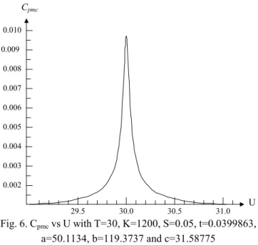
_U= 0.086 mm. Substitute these values into (12), (13), (14), and (15), to proceed the following discussion.

The optimal Cpmc*is 0.0019. The optimal process mean U*

is 30.0000 mm and the process tolerance t*is 0.05 mm. Figs. 5 and 6 show that when the process mean is located at the target with fixed tolerance value, the maximum Cpmand Cpmccan be

reached. The explanation is discernable by looking into the common expression, (U8T)2, in the denominator of (7) and (15). On the other hand, in Fig. 7, with fixed process mean at the target value, the maximum value Cpm, which is infinite, is

reached when t is near to zero and the maximum Cpmc, which is

finite, arrives when t is 0.04. The same conclusions are derived by examining Figs. 7 and 8. The fact behind different optimal t values being found when the PCI is at its maximum, is comprehensible because the variance in Cpmc is cost related,

while the variance in Cpmis cost unrelated. The t value in Cpm

can be any small value regardless of the cost impact resulting from tolerance cost.

Table 2 Various Cpmcwhen Cpmis 1.2

(U,t) (50.00,12.50) (50.05,12.49) (51.00,12.13) (51.05,12.09) (52.00,10.96) (52.05,10.88)

Cpm 1.2000000 1.2000000 1.2000000 1.2000000 1.2000000 1.2000000

Cpmc 0.0345994 0.0346019 0.0356385 0.0357504 0.0394258 0.039727

0.0025 0.0030 0.0035 0.0040 0.0045

28 29

t

U

30 31

0.0015 0.0050 0.0055 0.0060

Fig. 4. Feasible range for various combination of U and t with T=30, S=0.05, and P =3 when Cpm=1.2

U

0.3 0.4 0.5 0.6 0.7

29.5 30.0

Cpm

30.5 31.0

0.2 0.8 0.9 1.0 1.1 1.2

0.003 0.004 0.005 0.006 0.007

29.5 30.0 30.5 31.0 U

0.002 0.008 0.009

0.010

Fig. 6. Cpmcvs U with T=30, K=1200, S=0.05, t=0.0399863,

a=50.1134, b=119.3737 and c=31.58775

5.00 7.50

0.02 0.04

t

0.06 0.10

2.50 10.00 12.50

Fig. 7. Cpmvs t with T=30, U=30, S=0.05, and P=3

t

0.0100 0.0105

0.02 0.04 0.06 0.08 0.0095

0.0110 0.0120

0.0090 0.0115 0.0125 0.0130 0.0135

Fig. 8. Cpmcvs t with T=30, K=1200, S=0.05, a=50.11345,

b=119.3737, and c=31.58775

'

-As discussed in the preceding section, a lower quality loss (better quality) implies a higher tolerance cost, and a higher quality loss (poorer quality) indicates lower tolerance cost. Hence, the design parameters must be adjusted to reach an economic balance between reduction in quality loss and tolerance cost, so that the cost effectiveness PCI expression, , is maximized. The model developed in the following illustration attempts to achieve this objective in the case of multiple quality characteristics.

Before model development, a functional relationship between the dependent variable/and independent variable should be identified and thoroughly understood. Based on this relationship, the resultant overall quality characteristic such as

/

σ

and /can be estimated from the set of individual quality

characteristics in both product and process. The proposed process capability index, for the multiple quality characteristics is:

0

2 2

1

6 [( ) ] ( )

' / / / '

% % %

σ =

− =

− + +

∑

(16)

where '5 is the total number of quality characteristics in a

product or process.

Assembly is the process by which the various components and sub8assemblies are brought together to form a completed product which is designed to fulfill a certain product function. Tolerance design as well as parameter design should be considered simultaneously, particularly when the aspects of quality loss, tolerance cost, minor maintenance cost, and major maintenance cost are included in the objective function of interest. Therefore, to ensure that the required functionality and quality of a product are met, a proper determination of process mean and process tolerance among the assembly components is of critical importance.

The assembly application shown in Fig. 9 is a classic gearbox assembly which consists of five components: X1, X2,

X3, X4, and X5. In this example M0is 5 and the assembly

chain vector is: Aj= [1,1, –1, –1, –1]; the assembly chain

describing the product quality value XYof interest is:

XY= X1＋X2– X3– X4– X5 (17)

Thus, the assembly chain in describing the resultant process mean of the product quality value XYof interest is:

UY= U1＋U2–U3–U4– U5 (18)

Associated process means that U1, U2, U3, U4, and U5, as well

as process tolerances t1, t2, t3, t4, and t5must be determined so

that the gap XYbetween the bushing and gearbox falls within

the specification limits, USL and LSL, where T1is 0.9 mm,

USL is 0.985 mm, and LSL is 0.825 mm. Let K be $1500. The P value for estimating the process variance is assumed to be 3. Table 3 provides the upper and lower process capability limits for each component. Table 4 provides the coefficients a, b, and c for the tolerance cost functions, which can be found based on actual data collected in factories and analyzed through a statistical regression method. Based on given conditions from these tables, the problem is formulated via one of the optimization techniques such as mathematical programming. The objective intends to find optimal parameter and tolerance values so that the Cpmcis maximized

U1*= 16.0121 mm, U2*= 18.0150 mm, U3*= 29.0056 mm,

U4*= 1.8078 mm, U5*= 2.3087 mm, t1*= 0.0140 mm, t2*=

0.0196 mm, t3* = 0.0240 mm, t4* = 0.0115 mm and t5* =

0.0107 mm, and Cpmc*= 0.003844.

For the purpose of comparison, a further study is carried with the same formulation except that objective function Cpmc

is replaced with the expression of Cp, Cpk, or Cpm. The results

along with the above outcomes are summarized in Table 5. Clearly, Cpmc mirrors relevant quality and cost sensitively

and is most applicable during the stage of product design. In other words, is an appropriate expression for application in the process capability analysis during off8line application; particularly, for product design and process planning at the stage of blueprint.

Table 3 Upper and lower process capability limits for component j

j tLj[mm] tUj[mm]

1 0.014 0.042

2 0.018 0.052

3 0.024 0.072

4 0.009 0.027

5 0.010 0.030

Table 4 Tolerance cost function coefficients

j aj bj cj

1 10.0045 1.0036 4.0773

2 12.0127 1.0189 6.0921

3 10.0045 1.0036 4.0773

4 5.0981 0.9871 7.6381

5 6.5690 0.7621 5.9331

x1 x2

x4

x5

xY

x3

Fig. 9. A classic gearbox

Table 5 PCI values under various quality loss coefficient K K

PCI 15 150 1500 15000 150000

Cpmc 0.003846 0.003844 0.003832 0.003728 0.003005

Cpm 1.865577 1.865577 1.865577 1.865577 1.865577

Cpk 0.874489 0.874489 0.874489 0.874489 0.874489

Cp 1.865577 1.865577 1.865577 1.865577 1.865577

V. CONCLUSION

In the past, in using conventional PCI for measuring the process consequence, designers normally establish the process mean close to the design target, and minimize the process variance to small process capability limits so that the PCI value will be maximized. This one8way attitude in establishment will drive the PCI value to be unusually high since conventional PCI expression lacks consideration of quality loss and production cost involved during variance reduction and mean adjustment. Moreover, these are some of the reasons that concurrent engineers suggesting that possible issues occurring in the production stages should first be considered at the time that the new product is developed. That can reduce the time span for introducing a new product onto

market, and increase the chance for obtaining a superior edge among competitors. Thus, the present research introduces a PCI measurement, Cpmc, for the process capability analysis, to

ensure that lower production cost and high product quality can be achieved at the earlier time of the blue print stage. As a result, an effective PCI for product life cycle becomes actualized. In this regard, a new PCI expression Cpmc is

APPENDIX. PROOF THE DEPENDENCE BETWEEN PROCESS MEAN AND PROCESS TOLERANCE

Case 1 – Single quality characteristic

The expansion of/ " #about the point by Taylor's series up to the first three terms is:

/ " # " # ) " – #" ( )

1

∂

∂ #)

1 2!

" – #*" ( )

1

∂ ∂

#)

ℜ

(19)

where

ℜ

is the remainder. Taking the expectation of (19), the outcome is

/ ,"/# " # )

1

2

2 2

( )

∂

∂

6" # ) ,"

ℜ

#

≈

" # )

1

2

2

2

( )

∂

∂

6" #

≈

" # )

1

2

2 2

( )

∂

∂

2

σ

where

σ

=

≈

" # )

1

2

2 2

( )

∂

∂

2

(

)

(20)

To have an approximate value of V(Y), consider the Taylor’s series expansion up to the first two terms. That is:

/ " #

" # ) " – #"

( )

1

∂

∂

# (21)

Then 2

/

σ

≈

V(Y) = V (" #) + V(" – #" ( )

1

∂

∂ #]) =

_∑

[

"

( )

1

∂

∂

#

*

σ

2

] (22)

Because

σ

= , (22) can be further arranged as: 2

/

σ

"

( )

1

∂

∂

#

* 2

(

)

(23)

Case 2 8 Mutiple quality characteristics

Extending the above derivation to the design factors; assuming X1, X2, ..., Xnare independent; such as Y = f(X1,

X2, ..., Xn); that is:

/ "X1, X2, ..., Xn#

"U1, U2, ..., Un# )

[

∑

" – #"

1 2 3

1 2 3

, , , ..., ( , , , ..., ) ∂ ∂ #]) 1 2!

[

.

∑∑

" – #" .– .#

"

1 2 3

2

1 2 3

, , , ...,

( , , , ..., )

.

∂

∂ ∂ #])

ℜ

(24)

/ ,"/#

"U1, U2, ..., Un# )

1

2

∑

[

1 2 3

2

1 2 3

2

, , , ...,

( , , , ..., )

∂

∂ 6" #]

) ,"

ℜ

#

≈

"U1, U2, ..., Un#

) 1

2

∑

[

1 2 3

2

1 2 3

2

, , , ...,

(

,

,

, ...,

)

∂

∂

6" #]

(25) Assuming the relationship between tolerance value and standard deviation is

σ

, (25) can be further expressed as:

/

≈

"U1, U2, ..., Un# )

1

2

∑

[

1 2 3

2

1 2 3

2 , , , ...,

(

,

,

, ...,

)

∂

∂

2

( ) ] (26)

To have an approximate value of V(Y), consider the Taylor’s series expansion up to the first two terms. That is:

Y = "X1, X2, ..., Xn#

"U1, U2, ..., Un# )

∑

[

" – #

"

1 2 3

1 2 3

, , , ...,

(

,

,

, ...,

)

∂

∂

#] (27)

Then 2

/

σ

≈

V(Y) = V ("X1, X2, ..., Xn#) +

V(

∑

[

" – #"

1 2 3

1 2 3

, , , ...,

( , , , ..., )

∂

∂ #])

=

∑

[

"

1 2 3

1 2 3

, , , ...,

(

,

,

, ...,

)

∂

∂

#

*

σ

2 ] (28) Because

σ =

t

P

, (28) can be further arranged as:

2

/

σ

∑

[

"

1 2 3

1 2 3

, , , ...,

(

,

,

, ...,

)

∂

∂

#

*_{( )}2_]

(29) 2

/

∑

[

"

1 2 3

1 2 3

, , , ...,

(

,

,

, ...,

)

∂

∂

# * 2 ] (30) REFERENCES

[1] Boyle, R. A., "The Taguchi Capability Index," Journal of Quality Technology, Vol.23, 1991, pp.17826.

[3] Chase, K. W., Greenwood, W. H., Loosli, B. G., and Haugland, L. F., "Least Cost Tolerance Allocation for Mechanical Assemblies with Automated Process Selection," Manufacturing Review, Vol.3, No.1, 1990, pp. 49859.

[4] Carter, D. E. and Baker, B. S., , 2 27

-+ , - 8995. New York:

Addison8Wesley, 1992.

[5] Kane, V. E., "Process Capability Index," Journal of Quality Technology, Vol.18, 1986, pp.41852.

[6] Kotz, S. and Johnson, N. L., ! . London:

Chapman and Hall, 1993.

[7] Kotz, S. and Lovelace, C. R., !

-. London: Oxford University Press Inc-., 1998-.

[8] Jeang, A., "Economic Tolerance Design for Quality," Quality and Reliability Engineering International, Vol.11, No.2, 1995, pp.1138121.

[9] Jeang, A., "Combined Parameter and Tolerance Design Optimization with Quality and Cost Reduction," International Journal of Production Research, Vol.39, No.5, 2001, pp. 9238952.

[10]Jeang, A., Chung, C. P., and Hsieh, C. K., "Simultaneous Process Mean and Process Tolerance Determination with Asymmetric Loss Function," International Journal of Advanced Manufacturing Technology, Vol. 31, 2007, pp. 6948704..

[11]Phadke, M. S., , 2 2 2 : + 2 . New Jersey: Prentice Hall, Englewood Cliffs, 1989.

[12]Shina, S. G., "The Successful Use of the Taguchi Method to Increase Manufacturing Process Capability," Quality Engineering, Vol. 8, No. 3, 1991, pp.3338349.

[13]Taguchi, G. and Wu, Y.,! ; & .