Statistical downscaling of air temperature in the Douro Valley for agronomic applications

UNIVERSIDADE DE LISBOA

FACULDADE DE CIÊNCIAS

DEPARTAMENTO DE ENGENHARIA GEOGRÁFICA, GEOFÍSICA E ENERGIA

Statistical downscaling of air temperature in the Douro

Valley for agronomic applications

Andreia Filipa Silva Ribeiro

Dissertação

Mestrado em Ciências Geofísicas

Especialização em Meteorologia

FACULDADE DE CIÊNCIAS

DEPARTAMENTO DE ENGENHARIA GEOGRÁFICA, GEOFÍSICA E ENERGIA

Statistical downscaling of air temperature in the Douro

Valley for agronomic applications

Andreia Filipa Silva Ribeiro

Dissertação

Mestrado em Ciências Geofísicas

Especialização em Meteorologia

Dissertação orientada pela Doutora Susana M. Barbosa e co-orientada pelo Professor Pedro

Miranda

A Andreia Filipa Silva Ribeiro usufruiu de uma bolsa ANICT para o desenvolvimento da

Dissertação de Mestrado “

Statistical downscaling of air temperature in the Douro Valley for

“Começa por fazer o que é necessário, depois o que é possível e de repente estarás a

fazer o impossível”

À minha orientadora Doutora Susana Barbosa pela sua disponibilidade e apoio em vários momentos durante este Mestrado. O meu mais sincero agradecimento por todos os estímulos durante a orientação deste trabalho e por ter elevado os meus conhecimentos académicos e científicos, contribuindo para o meu crescimento pessoal e profissional. Nunca vou conseguir retribuir o constante incentivo e o testemunho pessoal que me serviram de inspiração e que tornaram possível a conclusão desta tese. Ao Professor e co-orientador Pedro Miranda pela oportunidade em trabalhar neste tema e pela oportunidade de me ter integrado no seu grupo de investigação. Agradeço igualmente todas as discussões e sugestões relevantes para este trabalho, que permitiram uma maior profundidade na interpretação dos resultados.

Ao Doutor Alexandre Ramos expresso a minha gratidão pela partilha dos dados das estações meteorológicas utilizados neste trabalho. Agradeço igualmente a disponibilidade e amabilidade na revisão dos primeiros resultados obtidos deste trabalho. A sua contribuição foi fundamental para este estudo.

À Doutora Rita Cardoso por disponibilizar os dados de reanálise e do modelo WRF e pelo auxílio prestado numa fase inicial do trabalho. As suas sugestões e recomendações foram de elevada importância para a realização desta tese.

Ao André Amaral e à Sofia Ermida, pela presença, pela força, pela amizade, e por me encorajarem sempre durante este Mestrado. As lágrimas e gargalhadas partilhadas não foram menos importantes para a conclusão deste curso.

A toda a minha família, em particular, aos meus pais, cujas palavras de coragem, apoio e amor incondicionais foram determinantes ao longo de todo o meu percurso académico e pessoal. À minha mana, por todo o carinho e doçura, e por ser sempre um motivo de alegria na minha vida.

A Deus, por mais um motivo de gratidão na minha vida. Obrigada por Seres fonte de inspiração e coragem em todos meus passos.

Agronomic activities are very dependent on local climatic conditions. The vineyard in particular is very sensitive to temperature, which significantly affects the composition of grapes and hence the final quality of the produced wine. In a climate change context knowledge of future temperature variability is important to minimize impacts and promote adaptation measures often entailing high costs. However, given the local character of agronomic activities, temperature projections are required at very small spatial scales, and downscaling of climate variables is therefore required. In this thesis temperature data from the high resolution (9km) meteorological model WRF and reanalysis data from ERA-interim are analyzed. Statistical downscaling techniques are applied to the ERA-interim data in order to obtain local temperature estimates for the wine producing region of the Douro valley. Several bioclimatic indices based on downscaled temperature are further calculated in order to evaluate the climatic potential of the Douro Wine Region.

Key-words: Statistical downscaling, Temperature, Bioclimatic indices, Douro Wine Region

Resumo

No contexto das alterações climáticas os impactos da variabilidade da temperatura têm sido um dos principais objectos de estudo ao longo do último século. A prática vitícola, em particular, é uma das actividades agronómicas mais influenciadas pela temperatura, e a sua importância económica para Portugal conduziu a vários estudos sobre este tópico. A Região Vinhateira do Douro constitui um excelente exemplo da contribuição dos produtores de vinho para o crescimento económico, e de como a complexa topografia da região contribui para a variabilidade climática, muitas vezes com consequências directas na qualidade final do vinho. Esta tese contribui para o conhecimento das condições climáticas locais da Região Vinhateira do Douro que influenciam a composição das uvas e a consequente qualidade do vinho produzido.

O impacto das alterações climáticas na qualidade do vinho da Região Vinhateira do Douro usando GCMs (General Circulation Models também conhecidos como Global Climate Models) e RCMs (Regional Climate Models) é discutido por vários autores. Contudo, a baixa resolução das grelhas dos GCMs, dos RCMs e da reanálise negligenciam aspectos regionais, e técnicas que permitam a obtenção de informação de menor escala surgem como um requisito essencial nas ciências agronómicas. A Região Vinhateira do Douro em particular é um excelente exemplo da necessidade de climatologia de alta resolução, motivada pela geomorfologia complexa da região. O objectivo deste trabalho é a realização de um downscaling estatístico da temperatura do ar para locais particulares de modo a focar em áreas localizadas da Região Vinhateira do Douro, com a intenção de poder ser aplicado no estudo de uma vinha em particular.

Existem vários métodos de downscaling com o propósito de colmatar o problema de baixa resolução dos GCMs e RCMs, que são geralmente subdivididos em duas categorias: downscaling dinâmico e estatístico. O downscaling dinâmico é uma abordagem numérica que consiste na utilização de modelos globais ou reanálise como forçadores de modo a obter simulações de dados mais detalhadas para uma região particular. O downscaling estatístico utiliza modelos estatísticos simples, de modo a estabelecer a relação estatística entre variáveis de grande escala e variáveis locais. Os modelos de regressão são bastante utilizados para downscaling estatístico destacando-se pelo seu custo computacional reduzido e a sua fácil aplicação.

Neste trabalho são consideradas três estações meteorológicas na Região Vinhateira do Douro, Vila Real, Pinhão e Régua, representando duas das três sub-regiões da Região Demarcada do Douro: Baixo Corgo (Régua e Vila Real) e Cima Corgo (Pinhão). Baixo Corgo é a sub-região que apresenta as temperaturas mais baixas devido à influência dos ventos do Atlântico, sendo protegida pelas serras do Marão e Montemuro, enquanto Cima Corgo apresenta temperaturas mais elevadas. Em contraste, a sub-região mais a este, Douro Superior, é a sub-região mais quente e mais seca e que tem as plantações de vinhas mais recentes, marcada por episódios de seca recorrentes. As estações

downscaling estatístico da temperatura do ar para a localização das estações. A suave topografia da reanálise ERA-Interim e do modelo WRF são ajustadas através de um gradiente de temperatura constante de 6ºC/km.

O downscaling estatístico realizado neste trabalho é baseado em métodos de regressão. Como pré-processamento na análise dos dados de temperatura é aplicada uma decomposição das séries temporais utilizando o método STL (Seasonal-Trend decomposition procedure based on Loess), um algoritmo iterativo e robusto baseado em regressão local. O ajuste sazonal das séries temporais é um passo fulcral para a análise de regressão e, neste trabalho, é obtido pela remoção da componente sazonal obtida pelo método STL.

Neste trabalho, a técnica de regressão baseada em mínimos quadrados ordinários é primeiro considerada, e posteriormente o método de regressão robusta é aplicado de modo a reduzir o impacto de eventuais outliers nos resultados. A relação estatística entre a reanálise/WRF e as observações é estabelecida a partir das séries temporais ajustadas sazonalmente para o período de calibração de 1989-2003. O downscaling estatístico da reanálise ERA-Interim e a combinação de downscaling dinâmico e estatístico do modelo WRF é realizado no período de validação de 2004-2006. O correspondente ciclo sazonal da reanálise ERA-Interim e do modelo WRF são adicionados posteriormente às séries temporais downscaled, dado que o ciclo sazonal médio é semelhante ao das observações. O ciclo sazonal das observações não é considerado neste trabalho dado que não seria possível a sua utilização no caso da aplicação desta técnica de downscaling para linhas temporais no futuro. De modo a avaliar o downscaling estatístico, quatro medidas de precisão estatística são utilizadas: o viés, a raiz do erro médio quadrático, o erro absoluto médio e o erro percentual absoluto. Como etapa final, as séries locais de temperatura obtidas por downscaling estatístico são utilizadas para avaliar o potencial climático para crescimento da uva, nas estações em estudo da Região Vinhateira do Douro. A caracterização do clima nesta região é realizada a partir de índices bioclimáticos baseados na temperatura durante o período de crescimento das videiras (Abril a Outubro). A temperatura média do período de crescimento (GST, Average growing season temperature) é calculada a partir da soma da média da temperatura média, durante os sete meses do período de crescimento. O índice GDD (Growing degree-days) corresponde à temperatura média acima de uma temperatura base de 10ºC, uma vez que não existe crescimento da uva abaixo desta temperatura, e permite descrever o tempo envolvido nos processos biológicos da videira. Semelhante a este último é o índice helio-térmico de Huglin (HI, Heliothermal Index of Huglin) que dá mais peso à temperatura máxima e considera um coeficiente de ajustamento devido à variação em latitude. A duração do período de crescimento é dada pelo LGS (Length growing season) que considera o número de dias em quem a temperatura média está acima dos 10ºC. O CI (Cool Nigth Index) é complementar ao HI e tem conta a média da temperatura mínima durante o período de maturação (Setembro). De acordo com os valores de cada índice é possível definir classes climáticas características do potencial climático de cada região.

Um dos principais resultados deste trabalho reside na excelente representação da variabilidade da temperatura máxima, mínima e média pelas séries temporais downscaled estatisticamente. De um modo geral, a regressão baseada em mínimos quadrados ordinários e a regressão robusta apresentam resultados semelhantes, indicando que o impacto de eventuais outliers não é significativo na variabilidade média. Verifica-se que o downscaling estatístico reduz significativamente as diferenças entre a ERA-Interim/WRF e as observações, revelando a importância do downscaling estatístico em aumentar a performance da reanálise ERA-Interim e do modelo WRF, e o valor adicional em combinar downscaling dinâmico e estatístico. Os índices bioclimáticos calculados a partir das séries downscaled estatisticamente destacam-se como sendo uma excelente aproximação dos índices calculados a partir das observações e constituem uma melhoria significativa do que se obteria a partir apenas da reanálise ERA-Interim e do modelo WRF. No que diz respeito à aplicação na vinha, o downscaling estatístico revela ser uma mais-valia ao capturar características locais, tal como a influência da altura das estações.

Palavras-chave: Downscaling estatístico, Temperatura, Índices bioclimáticos, Região

Vinhateira do Douro

Índice ... ix

1. Introduction ... 1

1.1 Agrometeorology and vineyard ... 1

1.2 Douro Valley case study ... 5

1.3 Climate downscaling ... 9

1.4 Goals and research objectives ... 13

2. Data and pre-processing ... 14

2.1 Observational data ... 14

2.2 WRF and ERA-Interim reanalysis data ... 16

2.3 Seasonal decomposition ... 19

2.3.1 Seasonal cycle ... 20

2.3.1 Seasonal adjustment ... 22

3. Methods ... 25

3.1 Ordinary linear regression ... 26

3.2 Robust regression ... 27

4. Results ... 28

4.1 Statistical downscaling of ERA-Interim reanalysis ... 28

4.2 Statistical downscaling of WRF model data ... 33

4.3 Application of statistically-downscaled data to viticulture ... 38

5. Discussion ... 44

6. Concluding remarks and future work ... 47

7. References ... 49

1. Introduction

During the last century the climate system has been suffering changes caused by human interference leading to increased vulnerability of various natural systems. Agronomic sciences have been facing major challenges in the last few years, trying to optimize systems and techniques to help endure and overcome climatic change impacts. Viticulture is one of the agronomic activities most directly influenced by climatic conditions and with high economic relevance for many countries, in particular Portugal. Recently, there has been an effort to bring together the scientific community and the wine-making sector to understand how climate affects wine production and quality and thus minimize the impacts and promote adaptation measures.

The Douro region is a good example of the importance of vineyards cultures to Portugal’s economic growth. Composed by a rugged terrain with a particular topography, this wine region was crafted giving rise a stunning stairway covered by vineyards that produce excellent wine grapes. Among other high quality wines, the Douro region produces the world famous Porto Wine that has the highest wine classification in Portugal, exerting a strong economic and cultural contribution. A combination of numerous factors contributes to this distinctive wine region, and climate characteristics are a key factor to understand the dynamics behind this high quality wine production. Understanding how temperature affects yield and the composition of grapes is important to assess the impacts in the final quality of the produced wine. In this context, the study of relationships between temperature and wine production is a bridge to quantify the effects of global warming and promote adaptive measures. Portugal, in particular the Douro region, is a fine example of the need of high resolution climatology, motivated by both geomorphologic complexity and large climate gradients. Downscaling techniques allow to obtain regional information, overcoming the problem of misrepresentation of small-scale features of the most widely used models for climate studies. In the next sub-chapter a literature review summarizing introductory concepts is followed by a brief overview of statistical downscaling techniques and its scientific motivation. Emphasis is given on the influence of climate variability in the vineyards of the Douro region, and climate scenarios associated to higher wine production.

1.1

Agrometeorology and vineyard

The importance of agriculture in human history arises when man began to domesticate animals and grow food, and soon realized that agriculture is dependent on climate. Particularly the characteristics of the Mediterranean climate make it unique in all climates of the world with both advantages and disadvantages for agriculture. Qualitatively the climate of the Portuguese territory is temperate with hot and dry summers, and rainfall concentrated in winter (see Koppen’s classification in “Atlas Climático Ibérico (1971-2000)”). Some major drawbacks for agriculture are the lack of rain during the

summer which limits the moisture available for plant growth, and excessive rains in winter that compromise the soils with poor drainage. However, these characteristics can be beneficial for some species, revealing to be favorable for a couple of agricultural practices. Vineyards are generally located in regions with climate as described above, in particular the most common species Vitis vinifera which requires long, warm-to-hot, dry summers and cool winters (Winkler et al. 1974). In fact, humid conditions are susceptible to certain fungus diseases causing vining plants to be poorly suited to humid summers, and long and dry summers are required for a desirable maturation of grapes (Mariano Feio, 1991). During the winter it is a plant with an extremely high resistance when faced with cold conditions, dying only with negative temperatures between -13º and -15ºC, which never happens in Portugal (Mariano Feio, 1991). Moreover, the consequences of climate change depend on the characteristics of each region and the capacity of grape varieties and producers to adapt (Jones et al. 2005).

In viticulture, climate is assessed differentiating three levels of climate: macroclimate, mesoclimate and microclimate (Smart and Robinson, 1991). While macroclimate refers to the climate of a region, extending over tens of kilometers depending on e.g. topography and distance from ocean, mesoclimate refers to a particular site, generally associated to a particular vineyard. Mesoclimate effects concern to e.g. sunlight, conditioning if vineyards are planted in hill-sides facing south or north in order to promote sunlight absorption. Microclimate is the climate within a surrounding plant canopy (above ground part of a particular vine), whose effects can occur over few centimeters. Using again the sunlight example, in the top of the canopy the sunlight may affect far more than in the center. Microclimate is appropriate when an individual vine is considered, while the climate of a vineyard is concerned with macroclimate or mesoclimate. In addition to the spatial scale, climate operates in temporal scales varying from broad to singular weather events, such as extreme weather events, manifested in temperature, precipitation and humidity parameters.

A set of climate conditions influence the grapevine depending on the region of viticulture, the most influential factor in growth of wine grapes being the temperature (Mullin et al. 1992), and generally temperatures of grapevine parts are at or near air temperature (Smart and Robinson, 1991). One effect of air temperature in the plant is water lost through transpiration: the higher the air temperature the most water is loss through transpiration, which enables to regulate the temperature of the leaf. The temperature has also a very important role in photosynthesis, varying with the stage of development of the grapes. Other factors, such as precipitation, radiation, humidity, fog, may also have effects, but much more limited (Winkler et al. 1974). In fact, although Vitis vinifera grows best in regions that have few or no summer rains, winter must be rainy in order to store water in the soil to carry vines through the summer, although irrigation can mitigate these deficiencies (Weaver, 1976).

Due to the important role of temperature in almost all biological aspects of the vine, knowledge of the developmental stages of the grapes is significant to understand how climate influences the different growth stages (Figure 1). Each year, the grapevine growth starts with the budburst corresponding to the growing point when the leaves are separated at the tip. After the budburst, the flowering begins, followed by the stage of fruit set where a grape berry begins to develop. The stage when grape berries start a color change and maturation is called véraison followed by the harvest that corresponds to the grape maturity. The grapes are then removed from the vine and are ready to begin the wine making process. The temperature largely influences the growing season length, which is crucial in the optimization of the maturation of grapes, determining the levels of sugar and the final wine (Jones et al. 2005). For many of the world benchmark regions, a study based on both climate and plant growth shows that high quality wine production is limited to 13 to 21ºC average temperatures during the growing season (Jones, 2006). Average temperatures higher than 21ºC are possible, but are mostly limited to fortified wines, table grapes and raisons (Jones and Alves 2012).

Figure 1 – Vegetative cycle of Vitis vinifera. Photos source: Sogrape Vinhos, S.A. (http:/ http://www.sograpevinhos.eu/)

The time between the different developmental stages of Vitis vinifera greatly depends on climate and geographic location (Jones and Davis 2000). In order to define climate regions more favorable to the development of grapes there are several bioclimatic indices based directly or indirectly on temperature during the growing season. Based on the values of each index it is possible to fit groups or classes varying from very cool to very hot regions characterizing the climatic potential of a geographic location. One of the earliest indices was intended to determine the time required for grapes to reach maturity, expressed by the total amount of heat received, yielding the concept of temperature-time values called degree days or heat units (Amerine and Winkler, 1944). Heat summation corresponds to the sum of the mean monthly temperature above 10ºC, since there is no growth below that temperature. Winkler et al. (1974) adopted this concept to the growing season (April 1 to October 31) at various locations in California and as a result it was classified into five regions according to heat summations values. Also called the Winkler index (WI), Jones et al. (2010) derived this variable for the western United States, classifying it as Growing Degree-Days (GDD), and a further Growing Season average Temperature index (GST) calculated by taking the average of the seven months of the growing season. With similar information, Malheiro et al. (2010) calculated the Length Growing

Season (LGS) as the number of days with mean temperatures above 10ºC, considering 182 days or higher an appropriate LGS for vine growing (Jackson, 2001).

Table 1 - Bioclimatic indices resumed in this work, their equations and references. Variables: GDD (Growing degree-days), GST (Average growing season temperature), LGS (Length growing season), HI (Heliothermal Index of Huglin), CI (Cool night index), DI (Dryness index),

HyI (Hydrothermic Index of Branas) and CompI (Composite Index).

Index Equation References (e.g.)

GDD (ºC)



Oct Apr

T

T ]/2) 10]

max[([ max min

Winkler (1974) Jones et al. (2010) Santos et al. (2012) GST (ºC)



Where N is the number of observations

Jones et al. (2010)

LGS

(days) Number of days with

T



10

º

C

Jackson (2001) Malheiro et. al. (2010)

HI



Where d is an adjustment for latitude

Tonietto and Carbonneau (2004) Malheiro et. al. (2010) Blanco-Ward et al. (2007)

Santos et al. (2012)

CI September averageT_min

Tonietto (1999) Malheiro et. al. (2010) Blanco-Ward et al. (2007) Santos et al. (2012) DI



Where

W

T

transpiration and

E

Riou et al. (1994) Tonietto and Carbonneau (2004)

Malheiro et. al. (2010) Blanco-Ward et al. (2007) Santos et al. (2012) HyI



Malheiro et. al. (2010) Blanco-Ward et al. (2007)

Santos et al. (2012)

CompI _{HyI ≥ 1400, DI ≥-100, HyI≤5100 and} Ratio of years combining 4 criteria:

min

T always ≥-17ºC

Malheiro et. al. (2010) Santos et al. (2012)

Similar to the heat summation concept, the classical Heliothermal Index of Huglin (HI) (Huglin, 1978) is widely used, giving more weight to maximum temperatures above mean temperatures and applying a coefficient which expresses the day-length adjustment due to latitude varying, which takes into account the average daylight period for the latitude studied (e.g., Tonietto and Carbonneau 2004, Jones et al. 2010, Malheiro et al. 2010). Complementary to HI is the Cool Night Index (CI) which provides a relative measure of maturation potential taking into account the minimum temperatures (mean of minima) during maturation period (September in the Northern Hemisphere and March for the Southern Hemisphere (Tonietto 1999)). This index allows to assess grape and wine qualitative potential, such as color and aroma, supplementing the Dryness Index (DI) which gives information about soil-water availability based on an adaptation of the potential water balance of Riou (Riou et al.

1994). HI, CI and DI combined define the Multicriteria Climatic Classification System (Géoviticulture MCC System) developed by Tonietto and Carbonneau (2004) for 97 grape-growing regions in 29 countries, among them Portugal. This system is a research tool for grape-growing and wine-making zoning, distinguishing 36 different climate types, recognized by Blanco-Ward et al. (2007) as a good method for viticultural zonation in the northwest of Spain, defining 6 climate types for that region. Assessing the potential risk of grapevine exposure to diseases is performed by the Hydrothermic Index of Branas (HyI) (Branas et al., 1946) combining the precipitation and temperature during the growing season by the sum of the product between the variables (e.g. Blanco-Ward et al. 2007, Malheiro et al. 2010). The risk is considered high if HyI exceeds 5100ºC.mm and low for values below 2500ºC.mm. The Composite Index (CompI), which provides the fraction of winegrowing optimal years in a specific time period, was developed by Malheiro et al. (2010), combining 4 criteria: HyI ≥ 1400, DI ≥-100, HyI≤5100 and T_minalways ≥-17ºC. A value of 0 corresponds to the total absence of suitable years, while a value of 1 means that all years are suitable for grapevine growing. More recently Santos et al. (2012) adapted this index by removing the Hydrothermic Index of Branas (HyI) criteria, since according to these authors it contributes to unrealistically low values of CompI for several established viticultural regions. The additional value of Santos et al. (2012) study was the update of information for viticultural zoning by mapping bioclimatic indices, and also the analyses of the inter-annual variability of the indices and possible long-trends, potentially related to large-scale atmospheric forcing.

1.2

Douro Valley case study

A combination of numerous factors such as topography, soil and Mediterranean climate characteristics contribute to the distinctive wine region of the Douro Valley. The Douro region produces the world famous Port Wine, among other high quality wines, achieving the highest wine classification as a denomination of controlled origin (DOC) in Portugal and has been classified by UNESCO (United Nations Educational, Scientific and Cultural Organization) as a World Heritage Site. It is a very rugged mountainous region situated in the province of Trás-os-Montes e Alto Douro in the northeastern Portugal, confined by the western mountains of Marão and Montemuro (Figure 2), which block the flow of moist air from the Atlantic Ocean (Fanet, 2004). The Douro River and its affluents (Figure 2), such as Tua and Corgo, extend into deep valleys and most crops are embedded in the river basins whose soils are mainly composed by schist that is beneficial to the longevity of the vines (Mayson, 2012). Many factors contribute to the unique Douro wines which are strong contributors to Portugal’s economy, thus understanding its production and how climate affects vineyards is of the highest importance, for the region and for the whole country.

Figure 2 – The Douro Wine Region topography, Douro River and main tributaries, and the location of the region within Portugal (top right). Identification of the three sub-regions: Below Corgo, Above Corgo and Upper Douro. The western high elevations correspond to the mountains of Marão and

Montemuro. Data source: IVDP (2011)

In order to improve the cultivation of vineyards and to safeguard the quality of wine, an administrative delimitation was marked in the Douro region, the Demarcated Region of Douro (DRD). Generally the DRD is characterized by hot and dry summers, followed by cool winters, thus governed by warm and dry conditions with heat and water stress in most years (Jones and Alves, 2012). According to the growing season average temperatures (GST) index for 1950-2000 the overall DRD is 65% a warm climate type, 24% an intermediate climate and nearly 10% hot climate type (ADVID (Associação para o Desenvolvimento da Viticultura Duriense), 2012). However, the complex topography of the Douro Valley promotes climate variability since the region extends over steep valleys at different solar exposures and different altitudes. Hence the distribution area of vineyards is not uniform and the DRD is usually subdivided into three sub-regions (Figure 1), from the west to the east, each one with its own mesoclimate: Below Corgo on the left margin of the River Corgo (west of DRD), Above Corgo on the right margin of the River Corgo (center of the DRD) and Upper Douro on the right margin of River Tua (east of DRD). Below Corgo is the coolest and rainy sub-region due to the influence of the Atlantic winds, while Above Corgo is a little warmer and drier (Mayson, 2012). In contrast, Upper Douro is the hottest and driest of the sub-regions and the most recently planted, marked by recurrent drought episodes (Mayson, 2012). This heterogeneous climate conditions are in agreement with the historic climate normal (1931-1960) describing generally wetter and cooler areas to the west in

more area as a warm climate type than the other two sub-regions, Above Corgo has more area as an intermediate climate type than the other two sub-regions and Douro Superior has twice the area in hot climate type than the other two regions on growing season average temperatures (GST) profile (ADVID, 2012). In addition Douro Superior has warmer maximum and minimum temperatures, on average, compared to the other sub-regions (ADVID, 2012).

To fully understand how climate parameters vary during the stages of growth of the grapes it is important to examine the evolution of the main stages of the vegetative cycle. In the DRD budburst typically occurs during March followed by flowering in May and véraison (coloring of the grapes) in July (Malheiro, 2005). In mid-August begins the evaluation of the maturation of the grapes to determine the start of the harvest that generally occurs in late September. In contrast with northwestern-Spain, where budburst occurs between April and June, delaying all the other stages compared to DRD (Lorenzo et al. 2012). Spring and early summer are the months of the most intensive growth period and the climate conditions of those seasons largely influence crop production and quality, being crucial for DRD wine production. Usually the time periods used for climate assessment in wine regions are the growing season (April-October) and dormant season (November-March). The historic climate normal (1931-1960) shows that maximum temperatures during growing season ranges from 22º4ºC to 30.3ºC (Table 2; ADVID, 2012).

Table 2 - Historic climate normal (1931-1960) statistics in the DRD for the growing season (April-October), dormant season (November-March) and annual values from 57 stations of

temperature. Adapted from ADVID (2012).

Variable Period Mean Median Std. Dev. Max. Min. Range Average Temperature (ºC) Annual 14.3 14.3 1.3 16.8 11.4 5.4 Growing Season 18.7 18.7 1.5 21.8 15.3 6.5 Dormant Season 8.1 8.2 1.1 10.0 5.1 4.9 Maximum Temperature (ºC) Annual 20.7 20.5 1.7 24.1 16.6 7.5 Growing Season 26.3 26.1 2.0 30.3 22.4 7.9 Dormant Season 12.8 12.6 1.5 15.4 8.4 7.0 Minimum Temperature (ºC) Annual 7.9 7.9 1.2 10.5 5.0 5.4 Growing Season 11.2 11.0 1.3 14.2 7.8 6.3 Dormant Season 3.4 3.4 1.1 6.0 1.1 4.9

Several authors provide information about the most favorable climatic conditions for wine production in the DRD during the different stages of the growth of grapes. According to Santos et al. (2012a) higher wine production in DRD is associated to wet and cool springs during budburst, and warmer conditions during flowering, noting that precipitation in March and high temperatures in May are favorable to yield. Similarly, other results show that high rainfall in March (budburst) and high temperatures and low precipitation in May (flowering) and June (véraison) favor grapevine yield (Santos et al., 2011).

The vegetative cycle is also a good indicator of favorable conditions for wine production. Vineyards exposed to an Atlantic Mediterranean climate exhibit a typical feature in their vegetative cycle characterized by a maximum of the photosynthetic activity at the end of spring and a minimum during winter (Gouveia et al., 2011). During the period of intense growth (budburst), in March, an increase in the photosynthetic activity is evident, starting to decrease in July. Gouveia et al. (2011) results indicate that lower photosynthetic activity in the previous autumn and the current spring, along with higher greenness during the summer, corresponds to a lower wine production.

Looking into the past decades, both maximum and minimum temperatures show increasing trends during the growing season, with similar changes in the annual mean (ADVID, 2012). This study of the longest available records, covering 1967-2010 for the DRD, shows that the years with the warmest minimum temperatures during the growing season were 2003 and 2006, and the years with the warmest maximum temperatures were 1995, 2006 and 2010. Winter exhibits a significant warming in minimum temperatures during 1967-2010, while no significant changes were observed in maximum temperatures. Other studies identified similar trends for Portugal, such as the increase in the daily mean temperature of 0.52ºC per decade since 1976 found by Ramos et al. (2011) based on 23 Portuguese stations. The inter-disciplinary studies about climatic changes for Portugal of Miranda et al. (2006) have shown an increase in minimum temperatures and a smaller rise in maximum temperatures as well. However, correlations between annual, growing season and dormant season weather regimes and temperature in DRD are not significant. While weather regimes exhibit weak trends, the significant trends in annual, growing season and dormant season temperatures, point towards a general warming that is not significantly driven by regional circulation changes (ADVID, 2012). In contrast, Santos et al. (2011) showed a clear connection between large-scale atmospheric flow (composites of mean sea level pressure) and yield (NCEP/NCAR reanalysis parameters for precipitation and 2 m air temperature of March, May and June). Concerning the North Atlantic Oscillation (NAO), the correlation with winegrape production is little or none (Jones, 1997) probably due to the fact that NAO is largely a wintertime mechanism and its effects diminish over the growing season.

In particular, the last winery year of 2012 experienced changes in the evolution of the main vine growth stages and most of the territory was in state of severe drought. The report performed by ADVID noted a delay in the vegetative cycle with the beginning of flowering and véraison occurring two weeks later than average. During winter, minimum air temperature reached very low values, and from February to December it was the driest period of the last 40 years. In addiction, many studies on future climate conditions in the DRD found the occurrence of more extreme heat events and a decrease in cold events (Santos et al. 2011, Gouveia et al. 2011, Jones and Alves 2012).

The late 20th _{century has been characterized by a warming in wine producing regions that has been}

mostly beneficial for high-quality wine production, while in some cases the cause for better quality is the improvement of viticulture and enological practices (Jones et al., 2005). To assess the viticultural suitability of DRD, bioclimatic indices provide useful information, in particular the Huglin Index (1950-2000) which describes 50% of the territory as warm temperate climate for viticulture, 35% as temperate climate, 10% as warm climate, and 4% as cool climate for crops (ADVID, 2012). A viticultural zoning for Europe during 1950-2009 show that most areas of the Iberian Peninsula are suitable for wine production, although a warming is expected to occur according to the Winkler (WI) and the Huglin (HI) indices (Santos et al., 2012). Future projections of winegrape suitability across Europe show a Dryness Index (DI) pattern for southern Europe projected to become very dry, namely in southern Iberia (Malheiro et al., 2010). The results are found to be similar to the ADVID (2012) assessment using a single climate model (HADCM3) that predicts a warming increase based on the Average Growing Season Temperature (GST) index, increase of Growing Degree Days (GDD) and an increase of the warm temperate class, and the forthcoming of a warm class for the Huglin Index (HI). Despite the fact that an increase of warm and dry conditions during the growing season is associated with the risk of plant pathogens exposure, the Hydrothermal Index (HyI) pattern reveals that all areas with a Mediterranean climate in southern Europe (e.g. Portugal, Spain and Italy) present low risk of contamination of diseases in vines, both in present and in future scenarios (Santos et al. 2012, Malheiro et al. 2010). In contrast, the Composite Index (CompI) predicts negatives effects in southern Europe regions, namely the Douro Valley. European Huglin Index (HI) patterns describe a northward extension of the wine-producing potential areas, since long day-lengths compensate the lower temperatures, leading to a northward extension of the viticultural zones (Malheiro et al., 2010). In addition a significant increase of the Cool Night Index (CI) with potential negative impacts in the Mediterranean Basin is predicted (Santos et al. 2012, Malheiro et al. 2010).

1.3

Climate downscaling

Climate models are typically the tools for modeling climate dynamics by simulating the interactions of the atmosphere, ocean and surface, based on the integration of physical, chemical, and sometimes biological equations. The coupled atmosphere-ocean models, General Circulation Models (GCMs, also known as a Global Climate Models) are widely used to understand the dynamics of the climate system, and generate future and past climate data. These computationally intensive numerical models are quite complex, and typically divide the planet in a 4-dimensional grid, by latitude, longitude, time and upward through the atmosphere. The spatial and temporal grid resolution indicates how detailed is the representation of information, depending on how large the grid cells are (in kilometers or degrees of latitude and longitude), how many vertical layers there are, and the size of the used time steps (how often calculations of the various properties occur).

The weather simulated by these models greatly depends on the assumed atmospheric concentration of greenhouse gases and different scenarios simulate different concentrations of gases. In IPCC (Intergovernmental Panel Climate Change) AR4 there were 40 different scenarios which are organized into six families, A1FI, A1B, A1T, A2, B1 and B2, each containing scenarios that are similar to each other. These scenarios came from the Special Report on Emissions Scenarios (SRES), in order to make projections of possible climate change making assumptions about the future e.g. technological development, economic growth, population increase, and thus estimating greenhouse gas concentrations.

Global climatological datasets are also built based on global atmospheric reanalysis such as the reanalysis from the European Centre for Medium Range Forecasts (ECMWF) or the reanalysis from the National Centers for Environmental Prediction (NCEP/NCAR). While GCMs do not necessarily use actual observations to generate initial conditions, reanalysis are generated from observations and assimilated data, providing a complete record of global atmospheric circulation. ERA-Interim is the latest global atmospheric reanalysis produced by ECMWF to replace the ERA-40 reanalysis and extend to the present date.

Models can be generated with higher or lower resolutions. GCMs and reanalysis operate with typical grid sizes of a few hundreds of kilometers, and thus are able to reproduce large-scale climate features. However, the low resolution of GCMs and reanalysis grid cells cannot resolve features on smaller scales, and regional aspects are overlooked. But information on smaller scales is required for the study of climate impacts since local climate change is largely influenced by local orography and other local parameters, which are not represented by a GCM. A way of solving this problem is to derive small scale information from a model or process with larger scale, which is known as downscaling technique.

There are several possible downscaling methods designed to fill this resolution problem, which are generally divided in two categories: dynamical and statistical downscaling. Dynamical downscaling is a numerical approach that consists in nesting a global model or reanalysis data to provide more detailed simulations for a particular location (Figure 3). Regional Climate Models (RCMs) are models with higher resolution than GCMs, which can be forced by GCMs or by reanalysis data, using those initial conditions to drive high resolution information. RCMs forced by ERA-40 reanalysis such as PRUDENCE and ENSEMBLES projects are valuable tools of atmospheric data for Europe, with resolutions ranging 25 and 50km. Recently Soares et al. (2012) proposed a regional climate dataset for the Portuguese mainland based on the Weather Research and Forecast Modeling System (WRF) model which was used to downscale ERA-Interim reanalysis trough two nested grids, one with 27 km and another with 9km of resolution.

The impact of climate change on wine quality using GCMs and RCMs is discussed by several authors. Santos et al. (2011) performed future grapevine yield projections for the Douro region using two GCM ensemble simulations, ECHAM5/MPI-OM1 with a spatial resolution of 1.875º for recent-past climate, and two integrations following the A1B scenario for future climate. COSMO-CLM was nested in ECHAM5 in order to obtain a finer-scale grid with 18km approximately, in a total of 3x5 grid-points in the Douro Valley. Santos et al. (2012) assessed climate change projections with 15 different GCM/RCM chains by dynamical downscaling: two ECHAM5/COSMO-CL simulations and 13 based on simulations of the ENSEMBLES project following the A1B scenario. Data from these simulations were extracted for the Douro Valley containing 3x4 grid-points of the ENSEMBLES project with 25km of resolution, and 4x7 grid points of the COSMO-CL simulations with 18km of resolution. Of even greater resolution is the global database WorldClim which is a result of several GCM’s output (http://www.worldclim.org) and incorporates weather station records providing monthly maximum and minimum temperatures and precipitation with ~1km of resolution. ADVID (2012) compared WorldClim data with records from Vila Real, Pinhão and Régua for 1967-2010 and found a high correlation between the station values and model indicating WorldClim adequacy. For future climate projections, downscaled models for the same grid of the WorldClim are used, interpolating the anomalies between the GCM and the baseline years of the WorldClim for three greenhouse emission scenarios, B2, A1B and A2 of the HADCM3 model.

Figure 3 – Schematic depiction of the Regional Climate Model nesting approach. Data source: World Meteorological Organization (WMO) (http://www.wmo.int)

Instead of spatial interpolation or nesting two models, statistical downscaling makes use of simple statistical models in order to establish the relationship between large-scale climate variables and local climate variables. A statistical downscaling model describes the functional relationship between a small scale variable y (predictand) and a large scale variable x (predictor):

f(x) =

y

(1)

A pre-requisite for statistical downscaling is the good representation of the predictor x by the climatic models and eq. (1) must be understood as a stochastic equation, which implies that different

predictands y are consistent with the same predictor x (von Storch, 1999). This statistical relationship is based on the fact that regional climate is governed by the large scale climate state x and local features y. Heyen et al. (1995) refer to downscaling as a term that describes a procedure in which information about a process with smaller scale is derived from a process with larger scale. The authors state four fundamental steps to perform downscaling: (1) identify a large scale parameter that governs the local parameter, (2) find the statistical relationship between the parameters, (3) validate the relationship with independent data and (4) given a successful validation the local parameter can be estimated from GCM results.

To determine the statistical relationship, a large number of downscaling techniques have been developed and generally good simulations from GCMs are chosen as predictors. Regression models are widely used for downscaling (e.g. Kilsby et al. 1997, Wilby et al. 1998, Schoof et al. 2001), since the focus of this statistical technique is to establish a relationship between a dependent variable and one or more independent variables. Among downscaling approaches, regression models stand out because they require much less computing power, and are easier to perform.

Other alternatives have arisen in response to the limitations of classic regression models. Tareghian et al. (2013) overstep some problems inherent in the standard regression models implementation by applying quantile regression (QR) instead. Their main motivation was the poor effectiveness of traditional linear regression models concerning different quantiles of the conditional distribution, rather than the mean. When the interest is in extreme events, standard regression models may fail to provide the desired information, but QR may overcome this limitation and produce more satisfactory results. In comparison with a standard regression model the QR performed by Tareghian et al. (2013) showed better performance and the functional relationship between predictor and predictand formulated by QR is clearer than by neural networks (Baur et al., 2004). In addiction Cannon (2011) developed a quantile regression neural network for downscaling.

Despite the popularity of multiple linear regression, other optional approaches, such as Artificial Neural Networks (ANN) (e.g. Schoof et al., 2001) have been applied and compared with regression based methods (e.g. Wilby et al. 1998, Schoof et al. 2001). Although ANNs are analogous to multiple regression in terms of describing a quantitative relationship between a predictand and a predictor, neural networks make no assumption about the form of the function or the degree of nonlinearity (Wilby et al., 1998) and in general the performance of neural networks is better than for multiple regression models (Schoof et al., 2001). Alternative models are based on Single Value Decomposition (SVD) (e.g. Widman et al., 2003) and Canonical Correlation Analysis (CCA) (e.g. Heyen et al. 1995, von Storch 1999) which involve different technical details like filtering predictors and predictands or the use of Principal Component Analysis (PCA) (e.g. Palatella et al. 2010).

The aim of conventional downscaling methods is to derive information about regional processes from large scale processes which generally implies that while involved variables are not the same, the predictor governs the predictand. In fact, the main objective is precisely to describe the link between those different features. However, sometimes it is also convenient to estimate local features assuming that predictor and predictand fields are the same climate variable, for instance, precipitation. Widman et al. (2003) compared standard downscaling methods using a 1000 hPa geopotential and simulated precipitation as a predictor field: while the geopotential predictor was able to predict about 30% of the observed monthly precipitation variance, models using simulated precipitation as a predictor explained over 60% of the observed monthly precipitation variability. Maak et al. (1997) investigated if it is possible to link a climatological parameter with a non-meteorological parameter such as phenological state of a plant. The authors used canonical correlation analysis (CCA) to derive a downscaling model capable to reproduce flowering date anomalies of Galanthus nivalis L. based on GCM air temperature

data. More recently Abatzoglou et al. (2012) developed statistical downscaling techniques for wildfire applications by tracking fire danger indices. The variety of possible applications of the downscaling methodology highlights its importance for climate studies and suggests that there must be an ongoing effort in the improvement of these techniques and their application to Agrometeorology.

1.4

Goals and research objectives

The purpose of this work is to obtain local temperature estimates for the wine producing region of the Douro valley since temperature is a key factor to understand the link between climate conditions and vineyards. In this thesis, temperature data from the high resolution 9km meteorological model WRF, reanalysis data from ERA-interim and local observations recorded at the meteorological stations of Vila Real, Pinhão and Régua are analyzed. First, ERA-Interim reanalysis is used to perform a statistical downscaling of temperature to the stations points. Second, an evaluation of dynamical downscaling is performed by comparing the 9km WRF model temperature simulations to observational data. Third, dynamical and statistical downscaling are combined by statistically downscaling the 9km WRF simulations to stations points. Furthermore, to classify the climatic potential of the Douro Wine Region to the vine growing, several bio-climatic indices based on downscaled temperature values are analyzed.

In the next chapter the meteorological variables and the corresponding pre-processing are described. The following chapter is entirely devoted to the methodology for statistical downscaling and validation applied in this work. The fourth chapter presents the major results of the analysis and in the last chapter a summary of the results is presented followed by final considerations.

2. Data and pre-processing

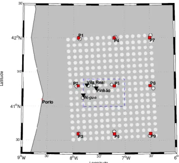
The Demarcated Region of the Douro (DRD) extends through the valley of the Douro River from about 100km upstream from Porto, to the border with Spain. A selected area within the DRD is typically considered to delimit the area of vineyards of the Douro region named the Douro Valley between 41.0-41.4ºN latitude and 7.0-7.8W longitude (Figure 4, blue dashed box) (Santos et al. 2011). For the current regional study an area between 40.5-42.0ºN latitude and 6.4-8.1ºW longitude is considered covering a significant network of available grid points of reanalysis, WRF model and meteorological stations (Figure 4).

Figure 4 – Map of the Douro Valley sector (blue dashed box), including the 9 grid points of ERA-Interim reanalysis (red), the 270 grid points of the WRF model simulation (white, black border denotes

the grid-points closer to ERA-Interim grid-points and stations) and the location of the meteorological stations of Vila Real, Pinhão and Régua (black triangles).

2.1

Observational data

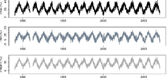
Three meteorological stations situated in the Douro Valley are considered: Vila Real, Pinhão and Régua (Table 3, Figure 4 black triangles). This study uses surface observations of daily Tmax and Tmin, recorded at 2m, already used by Ramos et al. (2011), and from these time series mean temperatures (Tmean) are calculated as Tmax+Tmin/2. Daily time series of Tmax, Tmin and Tmean from the meteorological stations of Vila Real, Pinhão and Régua, respectively, are displayed in Figure 5 to Figure 7 for the period 1989-2006. The observations are from the Instituto Português do Mar e da Atmosfera (IPMA) and are available for the period 1941-2006. Daily Tmax above 45 º C and below 0 º C and daily Tmin above 30 º C are set as missing, to avoid erroneous outliers. The time period 1989-2006 common to the WRF model and reanalysis data is considered. According to the applied criteria,

Pinhão and Régua present 0.02 and 0.03% (Table 3) of missing values while Vila Real remains nearly complete.

Table 3 - Characteristics of the meteorological stations considered in the Douro Valley.

Station Lat. (ºN) Lon. (ºW) Altitude. (m) Missing days (Tmax) Missing days (Tmin) Vila Real 41.32 7.73 481 1 0 Pinhão 41.27 7.55 65 128 130 Régua 41.17 7.80 130 190 189

Figure 5 – Daily maximum (top), minimum (center) and mean (bottom) temperature of Vila Real meteorological station for the period 1989-2006.

Figure 6 – Daily maximum (top), minimum (center) and mean (bottom) temperature of Pinhão meteorological station for the period 1989-2006.

Figure 7 – Daily maximum (top), minimum (center) and mean (bottom) temperature Régua meteorological station for the period 1989-2006.

2.2

WRF and ERA-Interim reanalysis data

This work uses a high resolution simulation of the WRF model, at 9km of horizontal resolution for the period of 1989-2008 corresponding to 18x15 grid points (Figure 4 white circles). Soares et al. (2012) proposed a regional climate dataset for the Portuguese mainland based on the WRF model, with a horizontal grid of 9km resolution, with the aim to use WRF as an RCM. In their study, the version 3.1.1 of the WRF model was used to downscale ERA-Interim reanalysis through two nested grids, one with 27 km and another with 9km of resolution. The outermost grid of 27 km resolution was forced in its interior by grid nudging, performed every 6 h at all levels above the planetary boundary layer, in order to mitigate problems in the propagation of large-scale features through boundaries of the model. Initial and boundary conditions for this outer domain were derived from the ERA-Interim reanalysis. The innermost 9 km resolution grid was performed by one-way nesting defined as a finer grid resolution driven by the coarse grid output as initial and boundary conditions. In a simplistic form, the coarser grid was forced by the atmospheric reanalysis, and the finer grid was forced by the output of the coarser grid. Both grids are centered in the Iberian Peninsula and the 27 km resolution grid domain covers a relatively large ocean area to reduce spurious boundary effects in the 9 km resolution domain. The present work uses the results of the WRF high resolution simulation of minimum and maximum temperatures that were previously evaluated against observations (Soares et al., 2012). Both 27 km and 9 km resolutions showed an improvement relatively to ERA-Interim on the representation of these parameters, but the finer grid was found to be generally better.

The ERA-Interim reanalysis data used by Soares et al. (2012) were interpolated to a regular grid of 0.7º of spatial resolution for the period of 1989-2008, and the same reanalysis data is used in the present study including 3x3 grid points in the study region (Figure 4). The smooth topography of the WRF model and reanalysis (Figure 8) requires a correction of temperature associated with altitude

differences, here adjusted trough a constant lapse rate of 6ºC/km applied to both maximum and minimum temperatures (Soares et al., 2012). This correction is applied for both grid points of WRF and ERA-Interim reanalysis data.

Figure 8 – Map of the Douro Valley (blue dashed box) and ERA-Interim reanalysis and WRF model topographies showing the western mountains of Marão and Montemuro.

Figure 9 – Schematic illustration of the altitude of the meteorological stations and of the ERA-Interim grid-point centered in the Douro Valley.

Figure 8 highlights the western mountains of Marão and Montemuro, which limit and shield the Douro Valley, the sixth and eighth higher elevations of Portugal, respectively. Since it is located in a less mountainous area than the closest grid-point, the ERA-Interim grid-point centered in the Douro Valley is considered henceforth for the analysis. The ERA-Interim closest grid-point is situated neighboring to Serra do Marão (Figure 8) becoming more difficult to represent local temperature due to the complex topography. The complex terrain of the Douro Valley makes the three meteorological stations network very distinct in altitudes with emphasis to Pinhão which is at very low altitude (Figure 9). The altitude of the ERA-Interim grid-point centered in the Douro Valley (672 m) is above all stations being closer to the altitude of Vila Real.

Figure 10 shows daily Tmax, Tmin and Tmean orography-corrected time series of reanalysis at the grid-point centered in the Douro Valley (Figure 4) for the available period 1989-2008. The same data for the WRF grid-point nearest to station of Vila Real is graphed in Figure 11 and both figures show similar seasonal cycles.

Figure 10 – Daily time series maximum (top), minimum (center) and mean (bottom) temperature of the ERA-Interim grid point within the Douro Valley (P5) for the period 1989-2008.

Figure 11 – Daily time series maximum (top), minimum (center) and mean (bottom) temperature of the WRF model grid point closer to Vila Real for the period 1989-2008.

Considering the available time period of observational data (1989-2006), WRF model and reanalysis data (1989-2008), the common period of 1989-2003 is considered for model calibration. The data for the period 2004-2006 are not used in the modeling stage being only used afterwards for validation purposes. Henceforth the 1989-2003 calibration period is considered.

2.3

Seasonal decomposition

As a pre-processing step in the analysis of temperature data, a time series decomposition is performed based on the STL method, the Seasonal-Trend decomposition procedure based on Loess and implemented in the R-package stl. The STL algorithm is based on locally-weighted regression, or loess (Cleveland et al., 1990), a robust method for curve estimation enabling STL to perform rather well even in the case of extreme observations and/or outliers. STL makes use of two smoothing parameters, one for the trend component and another for seasonality which controls how the seasonal component can change in time. Figure 12 illustrates the result of STL decomposition for Tmax at Vila Real using a seasonal smoothing parameter of 365 days. The time series (top) is decomposed from top to bottom into seasonal and trend components, and a remainder component corresponding to the residual variation of the data that is not modeled as seasonal or trend components. The STL decomposition implemented in the R-package stl requires time series with no missing values therefore gaps in observational records are replaced by interpolated values according to the algorithm of Stineman (1980) implemented in the R-package stinepack. After the decomposition, the interpolated values are again set as missing, and thus the resulting component time series have the same missing values as the original record.

Figure 12 – STL decomposition of the Vila Real maximum temperatures time series using a seasonal smoothing parameter of 365 days for the calibration period 1989-2003. From top to bottom: station records, seasonal component, trend component and remainder. The units on the vertical scales are in

2.3.1 Seasonal cycle

The mean seasonal cycle of temperature time series is obtained by averaging each calendar day over the whole 1989-2003 period and is shown for the three meteorological stations, the reanalysis grid-point centered in the Douro Valley and the WRF model closest grid-points in Figure 13. The mean seasonal cycle shows similar behavior for the three meteorological stations with Pinhão exhibiting slightly higher temperatures during summer.

The non-averaged seasonal cycle of Tmax, Tmin and Tmean resulting from the STL decomposition is shown for Vila Real in Erro! A origem da referência não foi encontrada.. The amplitude of the seasonal cycle is slightly larger for Tmax and Tmean than Tmin, and all seasonal cycles are apparently in phase. Annual amplitudes are computed as the difference between the maximum and the minimum of seasonal component for each calendar year and are approximately constant over the period 1989-2003.

Figure 13 – Tmax mean seasonal cycle of the meteorological stations records (black), reanalysis grid-point centered in the Douro Valley (gray) and WRF closest grid-point (slate gray) of Tmax (top) Tmin

Figure 14 - Seasonal component of the Vila Real station records (black), reanalysis grid-point centered in the Douro Valley (gray) and WRF closest point (slate gray) of Tmax (top) Tmin (center)

2.3.1 Seasonal adjustment

Seasonally adjusted temperature time series are obtained by removing the seasonal component derived by STL (previous section) and are shown for the Vila Real station in Figure 15. Seasonal adjustment is a crucial step before any regression analysis when the interest of the study is not on the seasonal cycle. Considering that the seasonal cycle is approximately constant trough the calibration period (Figure 13) only seasonally adjusted time series are considered in the analysis hereafter (Figure 15).

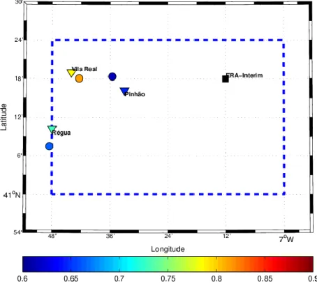
The bias between the seasonally-adjusted time series of the WRF model grid-cell and the observations are illustrated for the daily Tmin in Figure 16 for the calibration period 1989-2003. Generally the higher biases correspond to steeper topography areas (Figure 8, section 2.1) and the grid-points around the stations have smaller biases. Correlations and bias of seasonally-adjusted station data and the reanalysis grid-point centered in the Douro Valley and WRF closest point are shown in Table 4. Pinhão exhibits weaker correlations than the other stations possibly due to local effects not reproduced by the models. Both WRF and ERA-Interim seasonally adjusted time series tend to display higher bias at Vila Real, the station with highest altitude. At Pinhão and Régua WRF displays the smaller biases.

Table 4- Bias and correlation of seasonally-adjusted station data, ERA-Interim grid-point centered in the Douro Valley and WRF nearest points (confidence intervals in parenthesis).

Station/Point ERA-Interim WRF

Variable (ºC) Correlation Bias (ºC) Variable (ºC) Correlation Bias (ºC) Vila Real Tmax 0,79 (0,78-0,80) 2,71 Tmax 0,77 (0,76-0,78) 3,61 Tmin 0,81 (0,80-0,82) 2,80 Tmin 0,83 (0,82-0,84) 2,80 Tmean 0,86 (0,70-0,73) 2,76 Tmean 0,84 (0,83-0,85) 3,20 Pinhão Tmax 0,63 (0,61-0,64) -1,23 Tmax 0,62 (0,60-0,63) -0,20 Tmin 0,64 (0,62-0,65) 1,07 Tmin 0,58 (0,57-0,60) 0,86 Tmean 0,72 (0,71-0,73) -0,08 Tmean 0,68 (0,67-0,69) 0,33 Régua Tmax 0,77 (0,76-0,78) -1,02 Tmax 0,76 (0,75-0,78) 0,14 Tmin 0,80 (0,79-0,80) 0,31 Tmin 0,72 (0,71-0,73) -0,15 Tmean 0,84 (0,83-0,84) -0,36 Tmean 0,80 (0,79-0,81) -0,01

Figure 15 – Seasonally adjusted time series of the Vila Real station records (black), reanalysis grid-point centered in the Douro Valley (gray and WRF closest grid-point (slate gray) of Tmax (top) Tmin

Figure 16 - Bias between the seasonally-adjusted daily Tmin time series of the WRF grid-cell (circles) and the observations for the calibration period (1989-2003). Map of the Douro Valley (blue dashed

3. Methods

An overview of the main steps of the applied downscaling methodology (Figure 17) is presented in this section. The statistical downscaling procedure starts from the seasonally-adjusted time series of the three stations records, of the ERA-Interim grid-point centered in the Douro Valley and of the closest grid-points of the WRF model. The seasonal cycle is assumed to be approximately the same at the station and the considered grid-points (see section 2.3.1) and is added after the downscaling to the simulated time series.

Figure 17 – Schematic overview of the applied downscaling methodology.

The relationship between the reanalysis/WRF model data and observational data is established during the calibration period (1989-2003) for Tmax, Tmin and Tmean. The statistical relationship is subsequently used on the reanalysis/WRF model data during the validation period (2004-2006) to obtain local temperature estimates for subsequent agronomical applications. The local simulated temperature data is then evaluated to the observations.

Statistical downscaling of temperature to the stations points is based on regression methods. The ordinary linear regression is first considered (section 3.1). Robust regression (section 3.2) is then applied in order to reduce the impact of eventual outliers in regression results. To evaluate the statistical downscaling, four statistical accuracy measures are used: the bias, the roots mean squared error (RMSE), the mean absolute error (MAE) and the mean absolute percentage error (MAPE) (Table 5).

Table 5- Bias, root-mean squared error (RMSE), mean absolute error (MAE) and mean absolute percentage error (MAPE) equations with ̂ representing the downscaled

temperatures, the observations and N is the number of records.

Error Equation BIAS ∑( ̂ ) RMSE √ ∑( ̂ ) MAE ∑|̂ | MAPE ∑ | ̂ |

As a final step, the downscaled temperature data are used for assessing the climatic potential of the Douro Wine Region to vine growing. The climate assessment is performed based on the following bioclimatic indices (see Table 1): GDD (Growing degree-days), GST (Average growing season temperature), LGS (Length growing season), HI (Heliothermal Index of Huglin) and CI (Cool night index).

3.1

Ordinary linear regression

Ordinary linear regression methods are very common in many branches of geophysical data analysis (e.g. Helsel and Hisch, 2002). Recalling the generic functional relationship (Eq. (1), section 1.3), in the present study, let y represent the observational station records, x represent the reanalysis or regional model data, and the error ε be the difference between the observed value of y and the linear model estimates. The functional relationship of Eq. (1) can be described by a simple linear regression model as:

(2)

The method of ordinary least squares (OLS) is a common statistical tool to estimate the regression coefficients by minimizing the sum of the squared differences between the observations and the regression line:

∑(

)

∑(

)

(3)

In matrix notation eq. (2) can be written as:

(4)

where y is an vector of observations, X an matrix of regression variables, β an vector of regression coefficients, and ε an vector of random errors. The ordinary least squares (OLS) estimator of β is then given by:

̂ (

)

_.

₍₅₎

3.2

Robust regression

Ordinary least squares (OLS) assume that the errors are normally distributed, and thus it is not robust to eventual outliers present in the data. In such circumstances, robust regression is a good alternative since it gives less weight to outliers, reducing their influence on the estimated model (e.g. Hampel, 1986).

A robust regression M-estimator minimizes the sum of the objective function ρ instead of minimizing the sum of the squared residuals:

∑ (

)

∑ (

)

(6)

). The estimating equations can be written as:

∑

(

)

(7)

The M-estimation is performed by the Huber’s method (Huber, 1981) using the rlm() command in the MASS R-Package. Since residuals cannot be found until the model is fitted, an iterative procedure is necessary. As a result, iteratively reweighted least squares are used:

1. Ordinary least squares (OLS) is fitted in order to find estimates of the regression coefficients. 2. The residuals are extracted and used to calculate initial estimates for the weights.

3. A weight function is solved for the initial OLS residuals.