Gender gap developments in tertiary education : a cross-country time-series analysis on European level

(1)

Gender Gap Developments in

Tertiary Education

- A cross-country time-series analysis on European level

Julia Plötz

Dissertation written under the supervision of Hugo Reis and Miguel Gouveia

Dissertation submitted in partial fulfilment of requirements for the MSc in Economics, at the Universidade Católica Portuguesa,

(2)

i

“

An investment in knowledge pays the best interest.”

(3)

(4)

iii

Abstract

During recent decades, a reversal of the gender gap in tertiary enrollment and a subsequent growing gap in favor of women could be observed in most industrial-ized countries. This dissertation shows developments of the female-male gender gap in tertiary educational enrollment and analyzes factors behind the widening female-male gap with time-series data on European level. The analysis is based on a model of educational investment, which suggests that gender differences in benefits and costs of tertiary education help to explain gender gaps in tertiary educational investment. Using a first difference model to ensure stationarity, we find that only gender differences in cognitive and non-cognitive skills, as mea-sured by PISA scores in levels and standard deviations, significantly correlate with the gender gap in tertiary educational enrollment. We further find significant differences across time and country subgroup. Whether levels or the dispersion of cognitive and non-cognitive skills have explanatory power varies with country subregions and with the type of the PISA score used (Math or Reading).

(5)

(6)

v

Resumo

Recentemente, na maioria dos países industrializados, verifica-se uma inversão da diferença de genéro nas matrículas no ensino superior e, subsequentemente, um crescimento da diferença em favor das mulheres. Esta tese expõe tendências recentes das diferenças de género mulher-homem no acesso ao ensino superior. Analisa ainda os factores que levam ao aumento das diferenças de género com dados de séries temporais de países europeus. A análise é baseada no mod-elo básico de investimento educativo que sugere que diferenças de género em benefícios e custos do ensino superior podem ajudar a explicar a evolução no investimento feito no ensino superior. Para garantir estacionaridade, usamos um modelo em primeiras diferenças e concluímos que apenas as diferenças em competências cognitivas e não-cognitivas, medidas pelas classificações de leitura do PISA (níveis ou dispersão), se correlacionam significativamente com as difer-enças de género no número de matrículas no ensino superior. Este resultado varia com o tempo e subgrupo de países. O poder explanatório dos níveis ou da dispersão de competências cognitivas e não-cognitivas varia consoante as sub-regiões dos países e a classificação das disciplinas do teste PISA.

(7)

(8)

vii

Acknowledgements

First of all, I want to thank my supervisor Professor Hugo Reis not only for all his invaluable support, guidance and patience during the thesis process, but also for his good teaching in the Economics of Education class, which deepened my interest in educational matters.

I further want to express my gratitude to Professor Miguel Gouveia for his help during the topic ﬁnding process and in the ﬁrst months of the thesis writing process.

I also want to thank Professor Pedro Raposo for his good teaching of Microe-conometrics, which allowed me to understand and familiarize myself more easily with econometric methods used in this dissertation.

In addition, I want to express my gratitude to my professors from Université Catholique de Louvain and Universidade Católica Lisbon who made my Master a great and valuable experience.

Last but not least, I thank Géraldine Carette, Professor Teresa Lloyd-Braga and the student affairs team for all their great administrative support during my time at UCL and UCP.

Not to forget, I send a huge shout-out to my friends and ﬂatmates in Lisbon and all over the world as well as to my family for their never ending support and cheering up whenever needed.

(9)

(10)

ix

List of Figures

3.1 Gross Enrollment in Tertiary Education Over Time . . . 10

3.2 Gross Enrollment in Tertiary Education Decade to Decade . . . 11

A.1 Share of Population (Age 25-29) With Tertiary Education Over

Time . . . 48 A.2 Labor Force Participation Rate Over Time . . . 49 A.3 Scatterplot of male gap of PISA reading scores vs.

female-male gap of PISA maths scores . . . 51 A.4 Scatterplot of female-male gap of GER vs. female-male gap of

labor force participation rate . . . 54 A.5 Scatterplot of female-male gap of GER vs. female-male gap of

"earnings premium" . . . 54 A.6 Scatterplot of female-male gap of GER vs. female-male gap of

life expectancy at birth . . . 55 A.7 Scatterplot of female-male gap of GER vs. Crude Divorce Rate . 55 A.8 Scatterplot of female-male gap of GER vs. share of the

popula-tion aged 45-59 with tertiary degree . . . 55

A.9 Scatterplot of female-male gap of GER vs. fertility rates . . . . 56

A.10 Scatterplot of female-male gap of GER vs. female-male gap in

foregone earnings . . . 56 A.11 Scatterplot of female-male gap of GER vs.female-male gap in

PISA reading scores . . . 56 A.12 Scatterplot of female-male gap of GER vs. female-male gap in

(13)

(14)

xiii

List of Tables

4.1 Costs and Beneﬁts of Tertiary Education as in Becker, Hubbard,

and Murphy (2010) . . . 15

5.1 Summary Statistics in Levels . . . 22

6.1 Baseline Regression (T=12; N=18) . . . 32

6.2 Subgroups by Time Period: 2003-2007 and 2008-2014 . . . 35

6.3 Subgroups by Region: Western European, Nordic, Southern European and Eastern European . . . 37

6.4 Adding "Earnings Premium" and Foregone Earnings . . . 39

6.5 Robustness Regression: Baseline With Enrollment Numbers Instead of Enrollment Ratios . . . 40

6.6 Robustness Regression: Baseline With PISA Math Scores and Reading+Math Average . . . 42

A.1 Gross Enrollment Ratio of Men and Women and its Change Over Time . . . 47

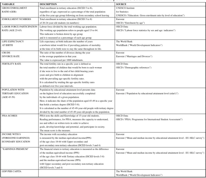
A.2 Variable Description and Source . . . 52

A.3 Summary Statistics in Levels (Country Subgroups) . . . 53

A.4 Summary Statistics in First Differences . . . 57

A.5 Summary Statistics in First Differences (Country Subgroups) . 58 A.6 Im, Pesaran and Shin Panel Unit Root Test . . . 59

(15)

(16)

1

1 Introduction

During recent decades, higher educational attainment grew rapidly in developed countries. Becker, Hubbard, and Murphy (2010) argue that a large part of this growth is caused by an increase in higher educational attainment of women. While more men than women used to be enrolled in and graduate from tertiary education decades ago, a stronger increase in educational attainment of women during recent decades led to convergence of female and male attainment patterns in most industrialized countries (Heath and Jayachandran, 2016). Data, disaggre-gated by gender, shows that educational attainment in industrialized countries did not only converge to relatively equal levels across genders, but female attain-ment continued to increase faster than male attainattain-ment. This allowed women to overtake men with respect to tertiary educational attainment and led to a positive and increasing female-male gender gap in higher educational attainment.

Authors such as Vincent-Lancrin (2008) argue that changing gender norms and tear-downs of societal restrictions for women can help to explain why women caught up with men in tertiary educational attainment. These factors, however, unlikely explain why women nowadays invest more in tertiary education than men do (Vincent-Lancrin, 2008).

The identiﬁcation of factors behind the widening of the gap in favor of women, however, is of great interest as changing educational gender patterns are expected to bring along important consequences for labor markets and societies: A positive and increasing female-male gender gap in tertiary educational attainment is expected to alter the skill composition in labor markets, which ultimately leads to a higher female share among advantaged high skilled workers and a higher male share among disadvantaged low skilled workers (Pekkarinen, 2012). The

(17)

2 Chapter 1. Introduction

author argues that these developments are of particular interest in current times, in which the importance of educational investments for labor market outcomes increases signiﬁcantly.

Since most industrialized countries experience similar developments in female-male gender gaps in tertiary education, it is interesting to analyze these develop-ments on a cross-country level. So far, there is little literature available which assesses the factors behind current developments in higher education qualita-tively and quantitaqualita-tively on a cross-country time-series level. Most existing literature follows either a descriptive approach or focuses its empirical analysis only on speciﬁc countries, such as Canada or the United States. Therefore, the aim of this dissertation is ﬁrst, to shed light on developments of the female-male gender gap in tertiary educational attainment in industrialized countries. Second, to outline empirically correlations of the gender gap with other socioeconomic developments.

Since individual investment decisions in education can be explained theoretically by a standard model of investment in tertiary education, in which individuals make investment decisions based on a cost-beneﬁt analysis of tertiary education, we use this model as a starting point for the analysis of gender gaps in educational attainment patterns in tertiary education. Thus, this dissertation will be based on an approach of Becker, Hubbard and Murphy (2010) who use the model of educational investment to analyze gender differences in tertiary educational attainment for the United States. Even though their model is a model of individual decision making, it will be adapted to aggregated country-level data.

The dissertation seeks to answer the following questions:

• Are gender differences in costs and beneﬁts of tertiary education correlated with gender differences in tertiary educational attainment in industrialized countries on aggregated level?

• Are there differences in correlations between country subgroups and over time sub-periods?

(18)

Chapter 1. Introduction 3

The study is based on a sample of the period 2003-2014 and 18 European countries consisting of the Nordic countries: Norway, Sweden, Denmark and Finland; the Western European countries: The Netherlands, Belgium, France, Ireland and Great Britain; the Southern European countries: Portugal, Spain, Greece and Italy and the Eastern European countries: Poland, Czech Republic, Hungary, Slovenia and Slovakia. All countries show a relatively high level of homogeneity and face similar gender gap developments over time. The empirical analysis uses a model in ﬁrst differences including time, year and GDP per capita as a country-year effect.

We do not intend to identify causalities, but rather correlations to make first indications about factors that accompany gender gap developments in tertiary education across countries. Hence, our findings can be used as first insights and a teaser for future research, but should not be used for policy recommendations. To better understand what lies behind each country’s behavior, specific country and richer data is desirable, which allows for a richer exploitation of correlations and causalities with respect to the model of individual investment in tertiary education.

The reminder of this dissertation is structured as follows: The next chapter gives a brief literature review. Chapter 3 shows educational attainment patterns over time for selected European countries. In chapter 4, the basic model of educational investment as developed by Becker, Hubbard, and Murphy (2010) is being presented on which the empirical analysis is based on. Chapter 5 describes the data sources and variables used for the empirical analysis. Chapter 6 outlines the econometric model and shows the results obtained from regressions. In chapter 7, potential shortcomings are discussed, suggestions for future research made and conclusions drawn.

(19)

(20)

5

2 Literature Review

Most existing literature on gender developments in tertiary education focuses either on single countries, such as the United States or Canada, or outlines potential factors behind developments of gender patterns over time only qual-itatively, but does not analyze them empirically. Thereby, authors often state that the catching up of women with men and their overtaking of men are not necessarily driven by the same factors (Vincent-Lancrin, 2008). Vincent-Lancrin (2008) looks at gender inequalities in higher education for OECD countries. The author concludes that the reversal of gender differences in tertiary educational participation and graduation rates is already well established across OECD coun-tries. Only on doctoral level and in the science ﬁeld does male participation still exceed female participation. According to the author, factors which could help to explain growing gaps in favor of women are potentially higher returns to tertiary education, higher professional aspiration of women, better non-cognitive skills of women as well as the feminization of the teaching profession and an increase in "female" courses during the educational expansion process.

A cross-country study which focuses more on the increasing gender gap in favor of women was conducted by Pekkarinen (2012). The author puts emphasis on a comparison between Nordic countries and the United States and uses a standard economic model of educational investment, in which investment decisions depend on the costs and beneﬁts of tertiary education, as a starting point for his analysis. The author concludes that increasing female-male gender gaps in education result from decreasing career restrictions for women in combination with higher returns to education for both genders and lower effort costs for women. The latter ones are caused by higher non-cognitive skills of women. Hence, following the author, there is a higher increase in net beneﬁts of education

(21)

6 Chapter 2. Literature Review

for women than for men.

Becker, Hubbard, and Murphy (2010) present a model where the distribution of costs and benefits of higher education across individuals determines the supply of college graduates in the market. The authors apply their analysis to US data only and, contrary to Pekkarinen (2012), do not find significant gender differences in the benefits of education. They show, in contrast, that gender differences in the distribution of non-cognitive skills lead to a higher elasticity of supply to college for women. This, in turn, allows female attainment to surpass male attainment even if changes in higher educational benefits are similar across the genders. Another study for the Unites States by Jacob (2002), which is based on longitu-dinal data, focuses on gender differences in average levels of financial returns to schooling and non-cognitive skills. The author shows that male students have lower grades and more advanced behavioral problems than female students. Jacob (2002) hence concludes that gender differences in non-cognitive skills, together with gender differences in returns to higher education, explain close to 90 percent of the female-male gender gap in higher educational attainment. Goldin, Katz, and Kuziemko (2006) confirm for the United States, that changing social norms, increased gender equality and changing expectations about the role of work, marriage and family planning allowed women to make better use of increasing educational and labor market benefits and hence incentivized them to increase their educational investment. Since these developments, as the authors argue, were accompanied by pronounced behavioral problems and slower social development of young men, women overtook men with respect to college attainment.

Again, for the United States, Buchmann and DiPrete (2006) examine whether the growing female-male gender gap with respect to college completion can be explained by either a gender-egalitarian hypothesis or by a gender-role hypoth-esis. The former assumes that higher average educational levels of parents are signiﬁcantly correlated with educational gender gaps in favor of women whereas

(22)

Chapter 2. Literature Review 7

the latter one states that changes in education or employment of mothers could have a greater impact on daughters than on sons and hence lead to trends in educational attainment in the detriment of men. Nevertheless, the authors do not ﬁnd evidence for any of the two hypotheses, but conclude instead that the recently growing female-male gender gap was caused by a decrease in attain-ment of young men whose fathers were absent or low-educated. In addition, the authors conﬁrm that better female behavior and performance allowed women to overtake men regardless of family backgrounds.

Buchmann, DiPrete, and McDaniel (2008) also present gender gaps for the United States and divide potential factors behind the differences in individual-level factors, such as family resources, academic achievements and returns to college and institutional factors, such as gender role attitudes, labor market factors, educational institutions and military service. Nevertheless, the authors do not analyze these factors empirically.

Christofides, Hoy, and Yang (2010) estimate gender differences in university participation rates for Canada by a linear probability and a logit model. The authors confirm the existence of a rising female-male enrollment gender gap in higher educational attainment. Using decomposition methods, they identify that gender gaps can be explained entirely by differences in variables, of which the university premium accounts for approximately 80%. Furthermore, the authors conclude that higher levels of college participation of both sexes are significantly correlated with changes in social norms, the university premium, tuition fees, real income and parent’s education.

Another single country analysis was conducted by Riphahn and Schwientek (2015) for Germany. The authors use a binary outcome model to estimate whether individual, labor market, institutional or demographic characteristics as well as changing norms can help to explain gender gaps in graduation from upper secondary school, entry to tertiary and completion of tertiary education. For gender gaps in tertiary education, the authors conclude that neither labor market factors nor family backgrounds help to explain developments over time.

(23)

8 Chapter 2. Literature Review

In contrast, decreasing class sizes as well as changes in social norms are said to positively inﬂuence female-male gender gaps in tertiary education.

(24)

9

3 Developments in Tertiary Educational

Attainment

In this dissertation, educational attainment will be measured by the gross en-rollment ratio (GER) for which data is available dis-aggregated by gender for a sufﬁciently long period and a cross section of countries. The was taken from the UNESCO Institute for Statistics where it is described as a measure of "total enrollment in tertiary education (ISCED 5 to 8), regardless of age, expressed as a percentage of the total population of the ﬁve-year age group following on from secondary school leaving". In other words, the GER is used to measure enrollment of students in school or university in comparison to the number of students who qualify for the particular grade level. It hence allows to show how enrollment increased over time, but also the difference in enrollment patterns between the sexes. The gross enrollment ratio includes over-age and under-age students and therefore often takes on relatively high values which can exceed 100%. This makes it a somewhat noisy measure of educational attainment. Nevertheless, as this dissertation focuses on gender differences rather than on absolute values of educational attainment, the GER is considered an adequate measure of educational attainment in the framework of this dissertation.

Figure 3.1 shows developments of female and male gross enrollment ratios for regional country groups (for a table with enrollment numbers by gender and their change from decade to decade see table A.1 in the appendix). It becomes apparent that different country groups started off with different gross enrollment ratios in 1975 for both genders, with Nordic countries showing the highest ratios and Eastern European the lowest. Over time, enrollment of both sexes increased signiﬁcantly, but female enrollment increased more rapidly than male enrollment:

(25)

10 Chapter 3. Developments in Tertiary Educational Attainment

Whereas in 1975, average gross enrollment was still signiﬁcantly higher among men than among women, already 20 years later, in 1995, the reverse was the case in all country groups under observation. Over time, the female GER continued to grow faster which led to an increase in the female-male gender difference of gross enrollment ratios.

Nevertheless, during the most recent decade, a change in patterns can be ob-served: First, the average female and male increase in enrollment ratios slowed down in all country groups and turned even negative in Nordic ones. This in-dicates that the countries under observation have already seen their strongest increase in tertiary educational expansion - at least for now. Second, in some country groups, this slowed down increase was more advanced for women than for men. This translates into a decreasing trend of the female-male gender gap in most recent years.

0 20 40 60 80 100 1970 1980 1990 2000 2010 Nordic Countries

male GER (%) female GER (%) female−male gender gap of GER

Year

Graphs by LOCATION

(a) Nordic Countries

0 20 40 60 80 100 1970 1980 1990 2000 2010

Western European Countries

Year

Graphs by LOCATION

(b) Western European Countries

0 20 40 60 80 100 1970 1980 1990 2000 2010

Southern European Countries

Year

Graphs by LOCATION

(c) Southern European Countries

0 20 40 60 80 100 1970 1980 1990 2000 2010

Eastern European Countries

Year

Graphs by LOCATION

(d) Eastern European Countries Figure 3.1: Gross Enrollment in Tertiary Education Over Time

(26)

Chapter 3. Developments in Tertiary Educational Attainment 11

From ﬁgure 3.1 we hence can summarize the following: 1. Enrollment of men and women increased over time

2. female enrollment increased faster than male enrollment, leading to a reversal of the enrollment gender gap

3. the increase in enrollment of men and women as well as of the female-male gender gap slowed down in most recent years

Let’s now take a closer look at developments by country. To do so, decade averages are plotted against each other for the decades 1975-1985 vs. 1985-1995 and 1995-2004 vs. 2005-2014 respectively (ﬁgure 3.2). This allows to determine increases or decreases of enrollment ratios and the development of the female-male gender gap over time on a more country speciﬁc level.

BEL BEL BEL BEL BEL BEL BEL BEL BEL BEL BEL BEL BEL BEL BEL BEL BEL BEL BEL BEL BEL BEL BEL BEL BEL BEL BEL BEL BEL BEL BEL BEL BEL BEL BEL BEL BEL BEL BEL BEL BEL BEL BEL BEL BEL BEL BEL BEL BEL BEL BEL BEL BEL BEL BEL CZE CZE CZE CZE CZE CZE CZE CZE CZE CZE CZE CZE CZE CZE CZE CZE CZE CZE CZE CZE CZE CZE CZE CZE CZE CZE CZE CZE CZE CZE CZE CZE CZE CZE CZE CZE CZE CZE CZE CZE CZE CZE CZE CZE CZE CZE CZE CZE CZE CZE CZE CZE CZE CZE CZE DNK DNK DNK DNK DNK DNK DNK DNK DNK DNK DNK DNK DNK DNK DNK DNK DNK DNK DNK DNK DNK DNK DNK DNK DNK DNK DNK DNK DNK DNK DNK DNK DNK DNK DNK DNK DNK DNK DNK DNK DNK DNK DNK DNK DNK DNK DNK DNK DNK DNK DNK DNK DNK DNK DNK ESP ESP ESP ESP ESP ESP ESP ESP ESP ESP ESP ESP ESP ESP ESP ESP ESP ESP ESP ESP ESP ESP ESP ESP ESP ESP ESP ESP ESP ESP ESP ESP ESP ESP ESP ESP ESP ESP ESP ESP ESP ESP ESP ESP ESP ESP ESP ESP ESP ESP ESP ESP ESP ESP ESP FIN FIN FIN FIN FIN FIN FIN FIN FIN FIN FIN FIN FIN FIN FIN FIN FIN FIN FIN FIN FIN FIN FIN FIN FIN FIN FIN FIN FIN FIN FIN FIN FIN FIN FIN FIN FIN FIN FIN FIN FIN FIN FIN FIN FIN FIN FIN FIN FIN FIN FIN FIN FIN FIN FIN FRA FRA FRA FRA FRA FRA FRA FRA FRA FRA FRA FRA FRA FRA FRA FRA FRA FRA FRA FRA FRA FRA FRA FRA FRA FRA FRA FRA FRA FRA FRA FRA FRA FRA FRA FRA FRA FRA FRA FRA FRA FRA FRA FRA FRA FRA FRA FRA FRA FRA FRA FRA FRA FRA FRA GBR GBR GBR GBR GBR GBR GBR GBR GBR GBR GBR GBR GBR GBR GBR GBR GBR GBR GBR GBR GBR GBR GBR GBR GBR GBR GBR GBR GBR GBR GBR GBR GBR GBR GBR GBR GBR GBR GBR GBR GBR GBR GBR GBR GBR GBR GBR GBR GBR GBR GBR GBR GBR GBR GBR GRC GRC GRC GRC GRC GRC GRC GRC GRC GRC GRC GRC GRC GRC GRC GRC GRC GRC GRC GRC GRC GRC GRC GRC GRC GRC GRC GRC GRC GRC GRC GRC GRC GRC GRC GRC GRC GRC GRC GRC GRC GRC GRC GRC GRC GRC GRC GRC GRC GRC GRC GRC GRC GRC GRC HUN HUN HUN HUN HUN HUN HUN HUN HUN HUN HUN HUN HUN HUN HUN HUN HUN HUN HUN HUN HUN HUN HUN HUN HUN HUN HUN HUN HUN HUN HUN HUN HUN HUN HUN HUN HUN HUN HUN HUN HUN HUN HUN HUN HUN HUN HUN HUN HUN HUN HUN HUN HUN HUN HUN IRL IRL IRL IRL IRL IRL IRL IRL IRL IRL IRL IRL IRL IRL IRL IRL IRL IRL IRL IRL IRL IRL IRL IRL IRL IRL IRL IRL IRL IRL IRL IRL IRL IRL IRL IRL IRL IRL IRL IRL IRL IRL IRL IRL IRL IRL IRL IRL IRL IRL IRL IRL IRL IRL IRL ITA ITA ITA ITA ITA ITA ITA ITA ITA ITA ITA ITA ITA ITA ITA ITA ITA ITA ITA ITA ITA ITA ITA ITA ITA ITA ITA ITA ITA ITA ITA ITA ITA ITA ITA ITA ITA ITA ITA ITA ITA ITA ITA ITA ITA ITA ITA ITA ITA ITA ITA ITA ITA ITA ITA NLD NLD NLD NLD NLD NLD NLD NLD NLD NLD NLD NLD NLD NLD NLD NLD NLD NLD NLD NLD NLD NLD NLD NLD NLD NLD NLD NLD NLD NLD NLD NLD NLD NLD NLD NLD NLD NLD NLD NLD NLD NLD NLD NLD NLD NLD NLD NLD NLD NLD NLD NLD NLD NLD NLD NOR NOR NOR NOR NOR NOR NOR NOR NOR NOR NOR NOR NOR NOR NOR NOR NOR NOR NOR NOR NOR NOR NOR NOR NOR NOR NOR NOR NOR NOR NOR NOR NOR NOR NOR NOR NOR NOR NOR NOR NOR NOR NOR NOR NOR NOR NOR NOR NOR NOR NOR NOR NOR NOR NOR POL POL POL POL POL POL POL POL POL POL POL POL POL POL POL POL POL POL POL POL POL POL POL POL POL POL POL POL POL POL POL POL POL POL POL POL POL POL POL POL POL POL POL POL POL POL POL POL POL POL POL POL POL POL POL PRT PRT PRT PRT PRT PRT PRT PRT PRT PRT PRT PRT PRT PRT PRT PRT PRT PRT PRT PRT PRT PRT PRT PRT PRT PRT PRT PRT PRT PRT PRT PRT PRT PRT PRT PRT PRT PRT PRT PRT PRT PRT PRT PRT PRT PRT PRT PRT PRT PRT PRT PRT PRT PRT PRT SVN SVN SVN SVN SVN SVN SVN SVN SVN SVN SVN SVN SVN SVN SVN SVN SVN SVN SVN SVN SVN SVN SVN SVN SVN SVN SVN SVN SVN SVN SVN SVN SVN SVN SVN SVN SVN SVN SVN SVN SVN SVN SVN SVN SVN SVN SVN SVN SVN SVN SVN SVN SVN SVN SVN SWE SWE SWE SWE SWE SWE SWE SWE SWE SWE SWE SWE SWE SWE SWE SWE SWE SWE SWE SWE SWE SWE SWE SWE SWE SWE SWE SWE SWE SWE SWE SWE SWE SWE SWE SWE SWE SWE SWE SWE SWE SWE SWE SWE SWE SWE SWE SWE SWE SWE SWE SWE SWE SWE SWE BEL BEL BEL BEL BEL BEL BEL BEL BEL BEL BEL BEL BEL BEL BEL BEL BEL BEL BEL BEL BEL BEL BEL BEL BEL BEL BEL BEL BEL BEL BEL BEL BEL BEL BEL BEL BEL BEL BEL BEL BEL BEL BEL BEL BEL BEL BEL BEL BEL BEL BEL BEL BEL BEL BEL CZE CZE CZE CZE CZE CZE CZE CZE CZE CZE CZE CZE CZE CZE CZE CZE CZE CZE CZE CZE CZE CZE CZE CZE CZE CZE CZE CZE CZE CZE CZE CZE CZE CZE CZE CZE CZE CZE CZE CZE CZE CZE CZE CZE CZE CZE CZE CZE CZE CZE CZE CZE CZE CZE CZE DNK DNK DNK DNK DNK DNK DNK DNK DNK DNK DNK DNK DNK DNK DNK DNK DNK DNK DNK DNK DNK DNK DNK DNK DNK DNK DNK DNK DNK DNK DNK DNK DNK DNK DNK DNK DNK DNK DNK DNK DNK DNK DNK DNK DNK DNK DNK DNK DNK DNK DNK DNK DNK DNK DNK ESP ESP ESP ESP ESP ESP ESP ESP ESP ESP ESP ESP ESP ESP ESP ESP ESP ESP ESP ESP ESP ESP ESP ESP ESP ESP ESP ESP ESP ESP ESP ESP ESP ESP ESP ESP ESP ESP ESP ESP ESP ESP ESP ESP ESP ESP ESP ESP ESP ESP ESP ESP ESP ESP ESP FIN FIN FIN FIN FIN FIN FIN FIN FIN FIN FIN FIN FIN FIN FIN FIN FIN FIN FIN FIN FIN FIN FIN FIN FIN FIN FIN FIN FIN FIN FIN FIN FIN FIN FIN FIN FIN FIN FIN FIN FIN FIN FIN FIN FIN FIN FIN FIN FIN FIN FIN FIN FIN FIN FIN FRA FRA FRA FRA FRA FRA FRA FRA FRA FRA FRA FRA FRA FRA FRA FRA FRA FRA FRA FRA FRA FRA FRA FRA FRA FRA FRA FRA FRA FRA FRA FRA FRA FRA FRA FRA FRA FRA FRA FRA FRA FRA FRA FRA FRA FRA FRA FRA FRA FRA FRA FRA FRA FRA FRA GBR GBR GBR GBR GBR GBR GBR GBR GBR GBR GBR GBR GBR GBR GBR GBR GBR GBR GBR GBR GBR GBR GBR GBR GBR GBR GBR GBR GBR GBR GBR GBR GBR GBR GBR GBR GBR GBR GBR GBR GBR GBR GBR GBR GBR GBR GBR GBR GBR GBR GBR GBR GBR GBR GBRGRCGRCGRCGRCGRCGRCGRCGRCGRCGRCGRCGRCGRCGRCGRCGRCGRCGRCGRCGRCGRCGRCGRCGRCGRCGRCGRCGRCGRCGRCGRCGRCGRCGRCGRCGRCGRCGRCGRCGRCGRCGRCGRCGRCGRCGRCGRCGRCGRCGRCGRCGRCGRCGRCGRC HUN HUN HUN HUN HUN HUN HUN HUN HUN HUN HUN HUN HUN HUN HUN HUN HUN HUN HUN HUN HUN HUN HUN HUN HUN HUN HUN HUN HUN HUN HUN HUN HUN HUN HUN HUN HUN HUN HUN HUN HUN HUN HUN HUN HUN HUN HUN HUN HUN HUN HUN HUN HUN HUN HUN IRL IRL IRL IRL IRL IRL IRL IRL IRL IRL IRL IRL IRL IRL IRL IRL IRL IRL IRL IRL IRL IRL IRL IRL IRL IRL IRL IRL IRL IRL IRL IRL IRL IRL IRL IRL IRL IRL IRL IRL IRL IRL IRL IRL IRL IRL IRL IRL IRL IRL IRL IRL IRL IRL IRL ITA ITA ITA ITA ITA ITA ITA ITA ITA ITA ITA ITA ITA ITA ITA ITA ITA ITA ITA ITA ITA ITA ITA ITA ITA ITA ITA ITA ITA ITA ITA ITA ITA ITA ITA ITA ITA ITA ITA ITA ITA ITA ITA ITA ITA ITA ITA ITA ITA ITA ITA ITA ITA ITA ITA NLD NLD NLD NLD NLD NLD NLD NLD NLD NLD NLD NLD NLD NLD NLD NLD NLD NLD NLD NLD NLD NLD NLD NLD NLD NLD NLD NLD NLD NLD NLD NLD NLD NLD NLD NLD NLD NLD NLD NLD NLD NLD NLD NLD NLD NLD NLD NLD NLD NLD NLD NLD NLD NLD NLD NOR NOR NOR NOR NOR NOR NOR NOR NOR NOR NOR NOR NOR NOR NOR NOR NOR NOR NOR NOR NOR NOR NOR NOR NOR NOR NOR NOR NOR NOR NOR NOR NOR NOR NOR NOR NOR NOR NOR NOR NOR NOR NOR NOR NOR NOR NOR NOR NOR NOR NOR NOR NOR NOR NOR POL POL POL POL POL POL POL POL POL POL POL POL POL POL POL POL POL POL POL POL POL POL POL POL POL POL POL POL POL POL POL POL POL POL POL POL POL POL POL POL POL POL POL POL POL POL POL POL POL POL POL POL POL POL POL PRT PRT PRT PRT PRT PRT PRT PRT PRT PRT PRT PRT PRT PRT PRT PRT PRT PRT PRT PRT PRT PRT PRT PRT PRT PRT PRT PRT PRT PRT PRT PRT PRT PRT PRT PRT PRT PRT PRT PRT PRT PRT PRT PRT PRT PRT PRT PRT PRT PRT PRT PRT PRT PRT PRT SVNSVNSVNSVNSVNSVNSVNSVNSVNSVNSVNSVNSVNSVNSVNSVNSVNSVNSVNSVNSVNSVNSVNSVNSVNSVNSVNSVNSVNSVNSVNSVNSVNSVNSVNSVNSVNSVNSVNSVNSVNSVNSVNSVNSVNSVNSVNSVNSVNSVNSVNSVNSVNSVNSVN SWE SWE SWE SWE SWE SWE SWE SWE SWE SWE SWE SWE SWE SWE SWE SWE SWE SWE SWE SWE SWE SWE SWE SWE SWE SWE SWE SWE SWE SWE SWE SWE SWE SWE SWE SWE SWE SWE SWE SWE SWE SWE SWE SWE SWE SWE SWE SWE SWE SWE SWE SWE SWE SWE SWE 10 20 30 40 50 1985−1995 10 20 30 40 50 1975−1985 Male Female equality

Female and Male Gross Enrollment Ratio (%)

(a) male and female 1975-1995 vs. 1985-1995

BEL BEL BEL BEL BEL BEL BEL BEL BEL BEL BEL BEL BEL BEL BEL BEL BEL BEL BEL BEL BEL BEL BEL BEL BEL BEL BEL BEL BEL BEL BEL BEL BEL BEL BEL BEL BEL BEL BEL BEL BEL BEL BEL BEL BEL BEL BEL BEL BEL BEL BEL BEL BEL BEL BEL CZE CZE CZE CZE CZE CZE CZE CZE CZE CZE CZE CZE CZE CZE CZE CZE CZE CZE CZE CZE CZE CZE CZE CZE CZE CZE CZE CZE CZE CZE CZE CZE CZE CZE CZE CZE CZE CZE CZE CZE CZE CZE CZE CZE CZE CZE CZE CZE CZE CZE CZE CZE CZE CZE CZE DNK DNK DNK DNK DNK DNK DNK DNK DNK DNK DNK DNK DNK DNK DNK DNK DNK DNK DNK DNK DNK DNK DNK DNK DNK DNK DNK DNK DNK DNK DNK DNK DNK DNK DNK DNK DNK DNK DNK DNK DNK DNK DNK DNK DNK DNK DNK DNK DNK DNK DNK DNK DNK DNK DNK ESP ESP ESP ESP ESP ESP ESP ESP ESP ESP ESP ESP ESP ESP ESP ESP ESP ESP ESP ESP ESP ESP ESP ESP ESP ESP ESP ESP ESP ESP ESP ESP ESP ESP ESP ESP ESP ESP ESP ESP ESP ESP ESP ESP ESP ESP ESP ESP ESP ESP ESP ESP ESP ESP ESP FIN FIN FIN FIN FIN FIN FIN FIN FIN FIN FIN FIN FIN FIN FIN FIN FIN FIN FIN FIN FIN FIN FIN FIN FIN FIN FIN FIN FIN FIN FIN FIN FIN FIN FIN FIN FIN FIN FIN FIN FIN FIN FIN FIN FIN FIN FIN FIN FIN FIN FIN FIN FIN FIN FIN FRA FRA FRA FRA FRA FRA FRA FRA FRA FRA FRA FRA FRA FRA FRA FRA FRA FRA FRA FRA FRA FRA FRA FRA FRA FRA FRA FRA FRA FRA FRA FRA FRA FRA FRA FRA FRA FRA FRA FRA FRA FRA FRA FRA FRA FRA FRA FRA FRA FRA FRA FRA FRA FRA FRA GBR GBR GBR GBR GBR GBR GBR GBR GBR GBR GBR GBR GBR GBR GBR GBR GBR GBR GBR GBR GBR GBR GBR GBR GBR GBR GBR GBR GBR GBR GBR GBR GBR GBR GBR GBR GBR GBR GBR GBR GBR GBR GBR GBR GBR GBR GBR GBR GBR GBR GBR GBR GBR GBR GBR GRC GRC GRC GRC GRC GRC GRC GRC GRC GRC GRC GRC GRC GRC GRC GRC GRC GRC GRC GRC GRC GRC GRC GRC GRC GRC GRC GRC GRC GRC GRC GRC GRC GRC GRC GRC GRC GRC GRC GRC GRC GRC GRC GRC GRC GRC GRC GRC GRC GRC GRC GRC GRC GRC GRC HUN HUN HUN HUN HUN HUN HUN HUN HUN HUN HUN HUN HUN HUN HUN HUN HUN HUN HUN HUN HUN HUN HUN HUN HUN HUN HUN HUN HUN HUN HUN HUN HUN HUN HUN HUN HUN HUN HUN HUN HUN HUN HUN HUN HUN HUN HUN HUN HUN HUN HUN HUN HUN HUN HUN IRL IRL IRL IRL IRL IRL IRL IRL IRL IRL IRL IRL IRL IRL IRL IRL IRL IRL IRL IRL IRL IRL IRL IRL IRL IRL IRL IRL IRL IRL IRL IRL IRL IRL IRL IRL IRL IRL IRL IRL IRL IRL IRL IRL IRL IRL IRL IRL IRL IRL IRL IRL IRL IRL IRL ITA ITA ITA ITA ITA ITA ITA ITA ITA ITA ITA ITA ITA ITA ITA ITA ITA ITA ITA ITA ITA ITA ITA ITA ITA ITA ITA ITA ITA ITA ITA ITA ITA ITA ITA ITA ITA ITA ITA ITA ITA ITA ITA ITA ITA ITA ITA ITA ITA ITA ITA ITA ITA ITA ITA NLD NLD NLD NLD NLD NLD NLD NLD NLD NLD NLD NLD NLD NLD NLD NLD NLD NLD NLD NLD NLD NLD NLD NLD NLD NLD NLD NLD NLD NLD NLD NLD NLD NLD NLD NLD NLD NLD NLD NLD NLD NLD NLD NLD NLD NLD NLD NLD NLD NLD NLD NLD NLD NLD NLD NOR NOR NOR NOR NOR NOR NOR NOR NOR NOR NOR NOR NOR NOR NOR NOR NOR NOR NOR NOR NOR NOR NOR NOR NOR NOR NOR NOR NOR NOR NOR NOR NOR NOR NOR NOR NOR NOR NOR NOR NOR NOR NOR NOR NOR NOR NOR NOR NOR NOR NOR NOR NOR NOR NOR POL POL POL POL POL POL POL POL POL POL POL POL POL POL POL POL POL POL POL POL POL POL POL POL POL POL POL POL POL POL POL POL POL POL POL POL POL POL POL POL POL POL POL POL POL POL POL POL POL POL POL POL POL POL POLPRTPRTPRTPRTPRTPRTPRTPRTPRTPRTPRTPRTPRTPRTPRTPRTPRTPRTPRTPRTPRTPRTPRTPRTPRTPRTPRTPRTPRTPRTPRTPRTPRTPRTPRTPRTPRTPRTPRTPRTPRTPRTPRTPRTPRTPRTPRTPRTPRTPRTPRTPRTPRTPRTPRT SVK SVK SVK SVK SVK SVK SVK SVK SVK SVK SVK SVK SVK SVK SVK SVK SVK SVK SVK SVK SVK SVK SVK SVK SVK SVK SVK SVK SVK SVK SVK SVK SVK SVK SVK SVK SVK SVK SVK SVK SVK SVK SVK SVK SVK SVK SVK SVK SVK SVK SVK SVK SVK SVK SVK SVN SVN SVN SVN SVN SVN SVN SVN SVN SVN SVN SVN SVN SVN SVN SVN SVN SVN SVN SVN SVN SVN SVN SVN SVN SVN SVN SVN SVN SVN SVN SVN SVN SVN SVN SVN SVN SVN SVN SVN SVN SVN SVN SVN SVN SVN SVN SVN SVN SVN SVN SVN SVN SVN SVN SWE SWE SWE SWE SWE SWE SWE SWE SWE SWE SWE SWE SWE SWE SWE SWE SWE SWE SWE SWE SWE SWE SWE SWE SWE SWE SWE SWE SWE SWE SWE SWE SWE SWE SWE SWE SWE SWE SWE SWE SWE SWE SWE SWE SWE SWE SWE SWE SWE SWE SWE SWE SWE SWE SWE BEL BEL BEL BEL BEL BEL BEL BEL BEL BEL BEL BEL BEL BEL BEL BEL BEL BEL BEL BEL BEL BEL BEL BEL BEL BEL BEL BEL BEL BEL BEL BEL BEL BEL BEL BEL BEL BEL BEL BEL BEL BEL BEL BEL BEL BEL BEL BEL BEL BEL BEL BEL BEL BEL BEL CZE CZE CZE CZE CZE CZE CZE CZE CZE CZE CZE CZE CZE CZE CZE CZE CZE CZE CZE CZE CZE CZE CZE CZE CZE CZE CZE CZE CZE CZE CZE CZE CZE CZE CZE CZE CZE CZE CZE CZE CZE CZE CZE CZE CZE CZE CZE CZE CZE CZE CZE CZE CZE CZE CZE DNK DNK DNK DNK DNK DNK DNK DNK DNK DNK DNK DNK DNK DNK DNK DNK DNK DNK DNK DNK DNK DNK DNK DNK DNK DNK DNK DNK DNK DNK DNK DNK DNK DNK DNK DNK DNK DNK DNK DNK DNK DNK DNK DNK DNK DNK DNK DNK DNK DNK DNK DNK DNK DNK DNK ESP ESP ESP ESP ESP ESP ESP ESP ESP ESP ESP ESP ESP ESP ESP ESP ESP ESP ESP ESP ESP ESP ESP ESP ESP ESP ESP ESP ESP ESP ESP ESP ESP ESP ESP ESP ESP ESP ESP ESP ESP ESP ESP ESP ESP ESP ESP ESP ESP ESP ESP ESP ESP ESP ESP FIN FIN FIN FIN FIN FIN FIN FIN FIN FIN FIN FIN FIN FIN FIN FIN FIN FIN FIN FIN FIN FIN FIN FIN FIN FIN FIN FIN FIN FIN FIN FIN FIN FIN FIN FIN FIN FIN FIN FIN FIN FIN FIN FIN FIN FIN FIN FIN FIN FIN FIN FIN FIN FIN FIN FRA FRA FRA FRA FRA FRA FRA FRA FRA FRA FRA FRA FRA FRA FRA FRA FRA FRA FRA FRA FRA FRA FRA FRA FRA FRA FRA FRA FRA FRA FRA FRA FRA FRA FRA FRA FRA FRA FRA FRA FRA FRA FRA FRA FRA FRA FRA FRA FRA FRA FRA FRA FRA FRA FRA GBR GBR GBR GBR GBR GBR GBR GBR GBR GBR GBR GBR GBR GBR GBR GBR GBR GBR GBR GBR GBR GBR GBR GBR GBR GBR GBR GBR GBR GBR GBR GBR GBR GBR GBR GBR GBR GBR GBR GBR GBR GBR GBR GBR GBR GBR GBR GBR GBR GBR GBR GBR GBR GBR GBR GRC GRC GRC GRC GRC GRC GRC GRC GRC GRC GRC GRC GRC GRC GRC GRC GRC GRC GRC GRC GRC GRC GRC GRC GRC GRC GRC GRC GRC GRC GRC GRC GRC GRC GRC GRC GRC GRC GRC GRC GRC GRC GRC GRC GRC GRC GRC GRC GRC GRC GRC GRC GRC GRC GRC HUN HUN HUN HUN HUN HUN HUN HUN HUN HUN HUN HUN HUN HUN HUN HUN HUN HUN HUN HUN HUN HUN HUN HUN HUN HUN HUN HUN HUN HUN HUN HUN HUN HUN HUN HUN HUN HUN HUN HUN HUN HUN HUN HUN HUN HUN HUN HUN HUN HUN HUN HUN HUN HUN HUN IRL IRL IRL IRL IRL IRL IRL IRL IRL IRL IRL IRL IRL IRL IRL IRL IRL IRL IRL IRL IRL IRL IRL IRL IRL IRL IRL IRL IRL IRL IRL IRL IRL IRL IRL IRL IRL IRL IRL IRL IRL IRL IRL IRL IRL IRL IRL IRL IRL IRL IRL IRL IRL IRL IRL ITA ITA ITA ITA ITA ITA ITA ITA ITA ITA ITA ITA ITA ITA ITA ITA ITA ITA ITA ITA ITA ITA ITA ITA ITA ITA ITA ITA ITA ITA ITA ITA ITA ITA ITA ITA ITA ITA ITA ITA ITA ITA ITA ITA ITA ITA ITA ITA ITA ITA ITA ITA ITA ITA ITA NLD NLD NLD NLD NLD NLD NLD NLD NLD NLD NLD NLD NLD NLD NLD NLD NLD NLD NLD NLD NLD NLD NLD NLD NLD NLD NLD NLD NLD NLD NLD NLD NLD NLD NLD NLD NLD NLD NLD NLD NLD NLD NLD NLD NLD NLD NLD NLD NLD NLD NLD NLD NLD NLD NLD NOR NOR NOR NOR NOR NOR NOR NOR NOR NOR NOR NOR NOR NOR NOR NOR NOR NOR NOR NOR NOR NOR NOR NOR NOR NOR NOR NOR NOR NOR NOR NOR NOR NOR NOR NOR NOR NOR NOR NOR NOR NOR NOR NOR NOR NOR NOR NOR NOR NOR NOR NOR NOR NOR NOR POL POL POL POL POL POL POL POL POL POL POL POL POL POL POL POL POL POL POL POL POL POL POL POL POL POL POL POL POL POL POL POL POL POL POL POL POL POL POL POL POL POL POL POL POL POL POL POL POL POL POL POL POL POL POL PRT PRT PRT PRT PRT PRT PRT PRT PRT PRT PRT PRT PRT PRT PRT PRT PRT PRT PRT PRT PRT PRT PRT PRT PRT PRT PRT PRT PRT PRT PRT PRT PRT PRT PRT PRT PRT PRT PRT PRT PRT PRT PRT PRT PRT PRT PRT PRT PRT PRT PRT PRT PRT PRT PRT SVK SVK SVK SVK SVK SVK SVK SVK SVK SVK SVK SVK SVK SVK SVK SVK SVK SVK SVK SVK SVK SVK SVK SVK SVK SVK SVK SVK SVK SVK SVK SVK SVK SVK SVK SVK SVK SVK SVK SVK SVK SVK SVK SVK SVK SVK SVK SVK SVK SVK SVK SVK SVK SVK SVK SVN SVN SVN SVN SVN SVN SVN SVN SVN SVN SVN SVN SVN SVN SVN SVN SVN SVN SVN SVN SVN SVN SVN SVN SVN SVN SVN SVN SVN SVN SVN SVN SVN SVN SVN SVN SVN SVN SVN SVN SVN SVN SVN SVN SVN SVN SVN SVN SVN SVN SVN SVN SVN SVN SVN SWE SWE SWE SWE SWE SWE SWE SWE SWE SWE SWE SWE SWE SWE SWE SWE SWE SWE SWE SWE SWE SWE SWE SWE SWE SWE SWE SWE SWE SWE SWE SWE SWE SWE SWE SWE SWE SWE SWE SWE SWE SWE SWE SWE SWE SWE SWE SWE SWE SWE SWE SWE SWE SWE SWE 20 30 40 50 60 70 80 90 100 2005−2014 20 30 40 50 60 70 80 90 100 1995−2004 Male Female equality

Female and Male Gross Enrollment Ratio (%)

(b) male and female 1995-2004 vs. 2005-2014

BEL BEL BEL BEL BEL BEL BEL BEL BEL BEL BEL BEL BEL BEL BEL BEL BEL BEL BEL BEL BEL BEL BEL BEL BEL BEL BEL BEL BEL BEL BEL BEL BEL BEL BEL BEL BEL BEL BEL BEL BEL BEL BEL BEL BEL BEL BEL BEL BEL BEL BEL BEL BEL BEL BEL CZE CZE CZE CZE CZE CZE CZE CZE CZE CZE CZE CZE CZE CZE CZE CZE CZE CZE CZE CZE CZE CZE CZE CZE CZE CZE CZE CZE CZE CZE CZE CZE CZE CZE CZE CZE CZE CZE CZE CZE CZE CZE CZE CZE CZE CZE CZE CZE CZE CZE CZE CZE CZE CZE CZE DNK DNK DNK DNK DNK DNK DNK DNK DNK DNK DNK DNK DNK DNK DNK DNK DNK DNK DNK DNK DNK DNK DNK DNK DNK DNK DNK DNK DNK DNK DNK DNK DNK DNK DNK DNK DNK DNK DNK DNK DNK DNK DNK DNK DNK DNK DNK DNK DNK DNK DNK DNK DNK DNK DNK ESP ESP ESP ESP ESP ESP ESP ESP ESP ESP ESP ESP ESP ESP ESP ESP ESP ESP ESP ESP ESP ESP ESP ESP ESP ESP ESP ESP ESP ESP ESP ESP ESP ESP ESP ESP ESP ESP ESP ESP ESP ESP ESP ESP ESP ESP ESP ESP ESP ESP ESP ESP ESP ESP ESP FIN FIN FIN FIN FIN FIN FIN FIN FIN FIN FIN FIN FIN FIN FIN FIN FIN FIN FIN FIN FIN FIN FIN FIN FIN FIN FIN FIN FIN FIN FIN FIN FIN FIN FIN FIN FIN FIN FIN FIN FIN FIN FIN FIN FIN FIN FIN FIN FIN FIN FIN FIN FIN FIN FINFRAFRAFRAFRAFRAFRAFRAFRAFRAFRAFRAFRAFRAFRAFRAFRAFRAFRAFRAFRAFRAFRAFRAFRAFRAFRAFRAFRAFRAFRAFRAFRAFRAFRAFRAFRAFRAFRAFRAFRAFRAFRAFRAFRAFRAFRAFRAFRAFRAFRAFRAFRAFRAFRAFRA GBR GBR GBR GBR GBR GBR GBR GBR GBR GBR GBR GBR GBR GBR GBR GBR GBR GBR GBR GBR GBR GBR GBR GBR GBR GBR GBR GBR GBR GBR GBR GBR GBR GBR GBR GBR GBR GBR GBR GBR GBR GBR GBR GBR GBR GBR GBR GBR GBR GBR GBR GBR GBR GBR GBR GRC GRC GRC GRC GRC GRC GRC GRC GRC GRC GRC GRC GRC GRC GRC GRC GRC GRC GRC GRC GRC GRC GRC GRC GRC GRC GRC GRC GRC GRC GRC GRC GRC GRC GRC GRC GRC GRC GRC GRC GRC GRC GRC GRC GRC GRC GRC GRC GRC GRC GRC GRC GRC GRC GRC HUNHUNHUNHUNHUNHUNHUNHUNHUNHUNHUNHUNHUNHUNHUNHUNHUNHUNHUNHUNHUNHUNHUNHUNHUNHUNHUNHUNHUNHUNHUNHUNHUNHUNHUNHUNHUNHUNHUNHUNHUNHUNHUNHUNHUNHUNHUNHUNHUNHUNHUNHUNHUNHUNHUN IRL IRL IRL IRL IRL IRL IRL IRL IRL IRL IRL IRL IRL IRL IRL IRL IRL IRL IRL IRL IRL IRL IRL IRL IRL IRL IRL IRL IRL IRL IRL IRL IRL IRL IRL IRL IRL IRL IRL IRL IRL IRL IRL IRL IRL IRL IRL IRL IRL IRL IRL IRL IRL IRL IRL ITA ITA ITA ITA ITA ITA ITA ITA ITA ITA ITA ITA ITA ITA ITA ITA ITA ITA ITA ITA ITA ITA ITA ITA ITA ITA ITA ITA ITA ITA ITA ITA ITA ITA ITA ITA ITA ITA ITA ITA ITA ITA ITA ITA ITA ITA ITA ITA ITA ITA ITA ITA ITA ITA ITA NLD NLD NLD NLD NLD NLD NLD NLD NLD NLD NLD NLD NLD NLD NLD NLD NLD NLD NLD NLD NLD NLD NLD NLD NLD NLD NLD NLD NLD NLD NLD NLD NLD NLD NLD NLD NLD NLD NLD NLD NLD NLD NLD NLD NLD NLD NLD NLD NLD NLD NLD NLD NLD NLD NLD NOR NOR NOR NOR NOR NOR NOR NOR NOR NOR NOR NOR NOR NOR NOR NOR NOR NOR NOR NOR NOR NOR NOR NOR NOR NOR NOR NOR NOR NOR NOR NOR NOR NOR NOR NOR NOR NOR NOR NOR NOR NOR NOR NOR NOR NOR NOR NOR NOR NOR NOR NOR NOR NOR NOR_PRT_PRT_PRT_PRT_PRT_PRT_PRT_PRT_PRT_PRT_PRT_PRT_PRT_PRT_PRT_PRT_PRT_PRT_PRT_PRT_PRT_PRT_PRT_PRT_PRT_PRT_PRT_PRT_PRT_PRT_PRT_PRT_PRT_PRT_PRT_PRT_PRT_PRT_PRT_PRT_PRT_PRT_PRT_PRT_PRT_PRT_PRT_PRT_PRT_PRT_PRT_PRT_PRT_PRT_PRT POLPOLPOLPOLPOLPOLPOLPOLPOLPOLPOLPOLPOLPOLPOLPOLPOLPOLPOLPOLPOLPOLPOLPOLPOLPOLPOLPOLPOLPOLPOLPOLPOLPOLPOLPOLPOLPOLPOLPOLPOLPOLPOLPOLPOLPOLPOLPOLPOLPOLPOLPOLPOLPOLPOL

SVN SVN SVN SVN SVN SVN SVN SVN SVN SVN SVN SVN SVN SVN SVN SVN SVN SVN SVN SVN SVN SVN SVN SVN SVN SVN SVN SVN SVN SVN SVN SVN SVN SVN SVN SVN SVN SVN SVN SVN SVN SVN SVN SVN SVN SVN SVN SVN SVN SVN SVN SVN SVN SVN SVN SWE SWE SWE SWE SWE SWE SWE SWE SWE SWE SWE SWE SWE SWE SWE SWE SWE SWE SWE SWE SWE SWE SWE SWE SWE SWE SWE SWE SWE SWE SWE SWE SWE SWE SWE SWE SWE SWE SWE SWE SWE SWE SWE SWE SWE SWE SWE SWE SWE SWE SWE SWE SWE SWE SWE −20 −10 0 10 20 1985−1995 −20 −10 0 10 20 1975−1985

Female−Male Gap of Gross Enrollment Ratio (pp) equality

Gender Gap Gross Enrollment Ratio (pp)

(c) gender gap 1975-1995 vs 1985-1995 BEL BEL BEL BEL BEL BEL BEL BEL BEL BEL BEL BEL BEL BEL BEL BEL BEL BEL BEL BEL BEL BEL BEL BEL BEL BEL BEL BEL BEL BEL BEL BEL BEL BEL BEL BEL BEL BEL BEL BEL BEL BEL BEL BEL BEL BEL BEL BEL BEL BEL BEL BEL BEL BEL BEL CZE CZE CZE CZE CZE CZE CZE CZE CZE CZE CZE CZE CZE CZE CZE CZE CZE CZE CZE CZE CZE CZE CZE CZE CZE CZE CZE CZE CZE CZE CZE CZE CZE CZE CZE CZE CZE CZE CZE CZE CZE CZE CZE CZE CZE CZE CZE CZE CZE CZE CZE CZE CZE CZE CZE DNK DNK DNK DNK DNK DNK DNK DNK DNK DNK DNK DNK DNK DNK DNK DNK DNK DNK DNK DNK DNK DNK DNK DNK DNK DNK DNK DNK DNK DNK DNK DNK DNK DNK DNK DNK DNK DNK DNK DNK DNK DNK DNK DNK DNK DNK DNK DNK DNK DNK DNK DNK DNK DNK DNK ESP ESP ESP ESP ESP ESP ESP ESP ESP ESP ESP ESP ESP ESP ESP ESP ESP ESP ESP ESP ESP ESP ESP ESP ESP ESP ESP ESP ESP ESP ESP ESP ESP ESP ESP ESP ESP ESP ESP ESP ESP ESP ESP ESP ESP ESP ESP ESP ESP ESP ESP ESP ESP ESP ESP FINFINFINFINFINFINFINFINFINFINFINFINFINFINFINFINFINFINFINFINFINFINFINFINFINFINFINFINFINFINFINFINFINFINFINFINFINFINFINFINFINFINFINFINFINFINFINFINFINFINFINFINFINFINFIN

FRA FRA FRA FRA FRA FRA FRA FRA FRA FRA FRA FRA FRA FRA FRA FRA FRA FRA FRA FRA FRA FRA FRA FRA FRA FRA FRA FRA FRA FRA FRA FRA FRA FRA FRA FRA FRA FRA FRA FRA FRA FRA FRA FRA FRA FRA FRA FRA FRA FRA FRA FRA FRA FRA FRA GBR GBR GBR GBR GBR GBR GBR GBR GBR GBR GBR GBR GBR GBR GBR GBR GBR GBR GBR GBR GBR GBR GBR GBR GBR GBR GBR GBR GBR GBR GBR GBR GBR GBR GBR GBR GBR GBR GBR GBR GBR GBR GBR GBR GBR GBR GBR GBR GBR GBR GBR GBR GBR GBR GBR GRC GRC GRC GRC GRC GRC GRC GRC GRC GRC GRC GRC GRC GRC GRC GRC GRC GRC GRC GRC GRC GRC GRC GRC GRC GRC GRC GRC GRC GRC GRC GRC GRC GRC GRC GRC GRC GRC GRC GRC GRC GRC GRC GRC GRC GRC GRC GRC GRC GRC GRC GRC GRC GRC GRC HUN HUN HUN HUN HUN HUN HUN HUN HUN HUN HUN HUN HUN HUN HUN HUN HUN HUN HUN HUN HUN HUN HUN HUN HUN HUN HUN HUN HUN HUN HUN HUN HUN HUN HUN HUN HUN HUN HUN HUN HUN HUN HUN HUN HUN HUN HUN HUN HUN HUN HUN HUN HUN HUN HUN IRL IRL IRL IRL IRL IRL IRL IRL IRL IRL IRL IRL IRL IRL IRL IRL IRL IRL IRL IRL IRL IRL IRL IRL IRL IRL IRL IRL IRL IRL IRL IRL IRL IRL IRL IRL IRL IRL IRL IRL IRL IRL IRL IRL IRL IRL IRL IRL IRL IRL IRL IRL IRL IRL IRL ITA ITA ITA ITA ITA ITA ITA ITA ITA ITA ITA ITA ITA ITA ITA ITA ITA ITA ITA ITA ITA ITA ITA ITA ITA ITA ITA ITA ITA ITA ITA ITA ITA ITA ITA ITA ITA ITA ITA ITA ITA ITA ITA ITA ITA ITA ITA ITA ITA ITA ITA ITA ITA ITA ITA NLD NLD NLD NLD NLD NLD NLD NLD NLD NLD NLD NLD NLD NLD NLD NLD NLD NLD NLD NLD NLD NLD NLD NLD NLD NLD NLD NLD NLD NLD NLD NLD NLD NLD NLD NLD NLD NLD NLD NLD NLD NLD NLD NLD NLD NLD NLD NLD NLD NLD NLD NLD NLD NLD NLD NOR NOR NOR NOR NOR NOR NOR NOR NOR NOR NOR NOR NOR NOR NOR NOR NOR NOR NOR NOR NOR NOR NOR NOR NOR NOR NOR NOR NOR NOR NOR NOR NOR NOR NOR NOR NOR NOR NOR NOR NOR NOR NOR NOR NOR NOR NOR NOR NOR NOR NOR NOR NOR NOR NOR POL POL POL POL POL POL POL POL POL POL POL POL POL POL POL POL POL POL POL POL POL POL POL POL POL POL POL POL POL POL POL POL POL POL POL POL POL POL POL POL POL POL POL POL POL POL POL POL POL POL POL POL POL POL POL PRT PRT PRT PRT PRT PRT PRT PRT PRT PRT PRT PRT PRT PRT PRT PRT PRT PRT PRT PRT PRT PRT PRT PRT PRT PRT PRT PRT PRT PRT PRT PRT PRT PRT PRT PRT PRT PRT PRT PRT PRT PRT PRT PRT PRT PRT PRT PRT PRT PRT PRT PRT PRT PRT PRT SVK SVK SVK SVK SVK SVK SVK SVK SVK SVK SVK SVK SVK SVK SVK SVK SVK SVK SVK SVK SVK SVK SVK SVK SVK SVK SVK SVK SVK SVK SVK SVK SVK SVK SVK SVK SVK SVK SVK SVK SVK SVK SVK SVK SVK SVK SVK SVK SVK SVK SVK SVK SVK SVK SVK SVN SVN SVN SVN SVN SVN SVN SVN SVN SVN SVN SVN SVN SVN SVN SVN SVN SVN SVN SVN SVN SVN SVN SVN SVN SVN SVN SVN SVN SVN SVN SVN SVN SVN SVN SVN SVN SVN SVN SVN SVN SVN SVN SVN SVN SVN SVN SVN SVN SVN SVN SVN SVN SVN SVN SWE SWE SWE SWE SWE SWE SWE SWE SWE SWE SWE SWE SWE SWE SWE SWE SWE SWE SWE SWE SWE SWE SWE SWE SWE SWE SWE SWE SWE SWE SWE SWE SWE SWE SWE SWE SWE SWE SWE SWE SWE SWE SWE SWE SWE SWE SWE SWE SWE SWE SWE SWE SWE SWE SWE −20 −10 0 10 20 30 40 50 2005−2014 −20 −10 0 10 20 30 40 50 1995−2004

Female−Male Gap of Gross Enrollment Ratio (pp) equality

Gender Gap Gross Enrollment Ratio (pp)

(d) gender gap 1995-2004 vs 2005-2014 Figure 3.2: Gross Enrollment in Tertiary Education Decade to Decade

(27)

12 Chapter 3. Developments in Tertiary Educational Attainment

Figure 3.2 (a) shows that average female as well as average male enrollment ratios were lower in the 1975-1985 than in the 1985-1995 period in all countries. One exception is Sweden in which average male enrollment decreased between the two decades while average female enrollment increased. A similar statement can be made for more recent decades (ﬁgure 3.2 (b)): Average enrollment of men and women, respectively, increased between the two decades, with the exception being Great Britain for which average male enrollment decreased. The graphs further show that female and male enrollment was more equally distributed in earlier decades (a) than in more recent ones (b) and show that female enrollment increased faster than male enrollment in all countries.

Figure 3.2 (c) and (d), which show the gender gap of enrollment ratios, conﬁrm these ﬁndings: While the decade averages of the female-male gender gap during the 1975-1985 period are still negative for most countries, and hence, male enrollment ratios exceeded female ones, they are positive during the 1985-1995 period for more than half of the countries. Hence, for most countries, a gender gap reversal had taken place between the two decades. Overall, the gender gap developed in favor of women in all countries under observation: Figure 3.2 (d) shows that the previously observed negative female-male gap had turned into a positive one in all countries. Again, in almost all countries the average of the female-male gender gap in the 1995-2004 period was lower than in the 2005-2014 period which indicates an increase in the female-male gender gap. The exceptions are Greece and Portugal where the average decade gap started to develop backwards again between 1995-2004 and 2005-2014.

A faster increase for women than for men and an increasing female-male gender gap can also be found for the share with tertiary degree among the 25-29 year old population as another measure of tertiary educational attainment (see ﬁgure A.1 in the appendix). The labor force participation rate of the 25-64-year-old population, however, shows that women did not yet fully catch up or overtake men with respect to labor market factors (see ﬁgure A.2 in the appendix).

(28)

13

4 Theoretical Considerations

After having shown that the female-male gender gap of tertiary educational enrollment increased signiﬁcantly over time, we present the model of educational investment in tertiary education by Becker, Hubbard and Murphy (2010) on which the empirical analysis will be based on. The equations presented in the following were one-to-one taken from the author’s paper.

4.1 Individual Decision Framework by Becker at al. (2010)

In the standard model of investment in education, rational individuals make their investment decisions in education based on a cost benefit analysis. Individuals with secondary degree only pursue further education, if benefits exceed costs or in other words if the net benefits are positive. Based on this model, Becker, Hubbard, and Murphy (2010) argue that gender differences in the marginal costs and benefits of tertiary education could help to explain why women caught up and surpassed men with respect to tertiary educational attainment.

The authors develop a model of investment in tertiary education in which they deﬁne the production of optimal investment as follows:

S_i= F(h, H, Ac,An) (4.1)

where H_i = initial human capital level; h = time spent in tertiary education; A_ci = cognitive skills; A_ni = non-cognitive skills. The ﬁrst derivatives of F(.) with respect to any of the input factors are positive, allowing for S to increase in all

(29)

14 Chapter 4. Theoretical Considerations

the inputs. At the optimal level of h, F_hh <0: The higher forgone earnings the higher the cost of h. F_hH,F_hA_c,F_hA_n > 0 holds: high skilled students (greater

A_c and/or A_n) need less time to produce the same S than low skilled students. The same holds for students with higher initial stock of human capital (higher H).

Individuals invest in period 1 and reap educational beneﬁts in period 2. Hence, optimal investment in tertiary education is chosen by maximizing discounted expected utility:

V = U1(x1,l; H) + p(S; H)βU2(x2,l2,S; H) (4.2)

subject to a budget constraint such that expected discounted consumption equals expected discounted income:

W = x1+ px₂ 1+ r+ w1l1+ p(S, H)w2l2 1+ r + T (h) + w1h = w1+ p(S, H)w2 1+ r + p(S, H)M(S) 1+ r (4.3)

Borrowing and lending takes place at rate r. β = discount rate; p(S;H) = prob-ability of surviving until period 2; x = consumption of goods; l = household time; W = full wealth (expected); w = earnings per hour; T = tuition and other fees; w₁h = foregone earnings and p(S)M(S) = gain from marriage (expected). p depends positively on H and S, reflecting the positive impact of education on health and specifically on chances of survival. U(.) is increasing in x,l,S and the total time in each period equals 1. The first derivatives of w₂ as well as M with respect to S are both greater than 0, reflecting the positive impact higher levels of education have on post-educational earnings and the higher gain from marriage for individuals with higher levels of education, respectively. Taking derivatives with respect to x₁, x₂, l₁ and l₂ and h ultimately leads to:

(30)

4.1. Individual Decision Framework by Becker at al. (2010) 15 p_SU₂ U_2x(1 + r) | {z } expected effect of higher survival prospects + pβU2S U_1x | {z } expected effect from future consumption + pSM+ pMS 1+ r | {z } expected effect of marriage beneﬁts + pS(w2e2− x2) 1+ r | {z } expected effect of higher survival probab. if if future earnings > future consumption + pw2Se2 1+ r | {z } expected effect of ﬁnancial returns to tertiary education = w1+ Th F_h | {z } marginal cost of additional unit of tertiary education (4.4)

(The derivations with respect to x₁,x2,l1,l2 can be found in the appendix).

Since this dissertation seeks to identify similarities across industrialized countries, data aggregated on country level is used. The model, however, is a model of individual decision making and is therefore more adequate for individual level data. To analyze correlations between gender gaps in tertiary enrollment and gender gaps in costs and beneﬁts with aggregated data, we adjust the model and depart from it whenever necessary.

Equation 4.4 shows that optimal investment in schooling depends on beneﬁts and costs of additional education, which can be grouped as follows:

Table 4.1: Costs and Beneﬁts of Tertiary Education as in Becker, Hubbard, and Murphy (2010)

Benefits Costs

LABOR MARKET BENEFITS: ﬁnancial returns DIRECT COSTS: tuition fees MARRIAGE MARKET BENEFITS: propensity to marry and stay married

HEALTH BENEFITS: higher survival prospects INDIRECT COSTS: foregone earnings and time spent at university (cognitive and non-cognitive skills)1

HOUSEHOLD PRODUCTION BENEFITS: effect of parent’s education on children’s education

We base the selection of explanatory variables on these ﬁve categories. We will not include tuition fees in our empirical analysis due to lack of data availability and based on the argumentation that tuition fees do not vary by gender and hence are unlikely to explain part of the gender gap’s variation in tertiary education (Becker, Hubbard, and Murphy, 2010). Furthermore, in most countries of our

(31)

16 Chapter 4. Theoretical Considerations

sample, tuition fees are non-existent or negligible and did not change signiﬁcantly during most recent decades.

4.1.1 Other Considerations

Table 4.1 shows the costs and beneﬁts of tertiary education as considered by Becker, Hubbard and Murphy (2010). Besides, we consider two other factors important for our analysis which could help to explain gender gap developments in tertiary educational attainment: labor market expectations and expectations about family planning.

Becker, Hubbard, and Murphy (2010) do not include labor market expectations in their analysis due to potential endogeneity problems. However, other authors, such as Goldin, Katz, and Kuziemko (2006),Vincent-Lancrin (2008) or Pekkari-nen (2012) consider labor market expectations an important factor for investment decisions in tertiary education and gender gap developments. Better labor mar-ket prospects increase the value of educational benefits, especially in times of increased demand for high-skilled workers and increased financial returns to educational investment (Pekkarinen, 2012). Goldin, Katz, and Kuziemko (2006) find for the US, that higher expectations of employment in the future worked as an incentive for women to invest in college education. Hence, similar develop-ments on cross-country level could help to explain gender gap developdevelop-ments in tertiary education

In addition to labor market expectations, a vast amount of literature considers changes in family norms and gender restrictions as potential explanations for the catching up of women. A decrease in discrimination of women, the possibility to postpone family planning and better possibilities to combine family with profes-sional life allow for higher female investments in tertiary education (Pekkarinen, 2012, Vincent-Lancrin, 2008). Even though such developments are more likely to be correlated with catching up of women, switching importance from family planning to career planning could help to explain why women nowadays invest

(32)

4.1. Individual Decision Framework by Becker at al. (2010) 17

more in education: if women expect to spend less time raising kids and more for work, they can better reap the beneﬁts of education.

(33)

(34)

19

5 Data Sampling and Variable Definition

5.1 Outcome Variable

We measure educational attainment as outcome variable by the Gross Enrollment Ratio in Tertiary Education (GER) which had already been presented in chapter 3. The GER is dis-aggregated by gender and data is available across countries and years which allows for the construction of a cross-section time-series dataset on aggregated level. Gender differences in educational attainment are calculated by subtracting male from female GERs by country and year respectively.

5.2 Explanatory Variables

We include the following variables as explanatory variables. 1. Labor Markets:

Gender Gap in Labor Force Participation Rate: We measure labor market expectations by the labor force participation rate of the population aged 25-64. Ideally, we would use the gender gap of a variable which measures the difference in labor force participation rates of the population with tertiary degree vs. secondary degree. However, due to lack of data, the labor force participation rate is used independently from educational degree.

Gender Gap in Earnings Premium (in logs): The ﬁnancial return to ter-tiary education is measured by the difference in the median equivalized income of the population aged 18-64 with tertiary degree versus the median

(35)

20 Chapter 5. Data Sampling and Variable Definition

equivalized income of the population aged 18-64 with secondary degree, for men and women respectively.

2. Health/Longevity:

Gender Gap in Life Expectancy at Birth: We measure survival prospects by the life expectancy at birth dis-aggregated by gender. It would be ideal to use life expectancy dis-aggregated also by educational level to measure the "health premium" of tertiary education. However, due to data restrictions, we rely on life expectancy at birth dis-aggregated by gender only.

3. Marriage Markets:

Crude Divorce Rate: Following the model by Becker, Hubbard and Mur-phy (2010) we would like to have data on marriage or divorce rates dis-aggregated by gender and educational level of individuals to perfectly capture gender differences in the "marriage market premium" of tertiary education. However, due to the aggregated structure of our data, we cannot capture marriage market beneﬁts as in the model. We thus depart from the model and measure marriage market factors by the overall crude divorce rate based on Pekkarinen (2012), who argues that increasing divorce rates act as an incentive for women to be ﬁnancially independent and hence to invest more in tertiary education.

4. "Household Production" Factors:

Population Share With Tertiary Education of Parent’s Age Cohort: To measure the effect of parent’s education on their son’s or daughter’s educa-tion on aggregate level, we proxy parent’s educaeduca-tion by the total share of the population aged 45 to 59 with tertiary degree.

Fertility Rates (in logs): We use fertility rates to reﬂect changes in the importance of family planning and women’s possibility to devote time to education and labor markets instead of family.

(36)

5.3. Summary Statistics 21

5. Costs of Education:

Gender Gap in Foregone Earnings (in logs): We measure foregone earn-ings by average annual income of the population with secondary education. Gender Gap in Cognitive and Non-Cognitive Skills: We use average PISA reading scores as well as their dispersion (standard deviation) to measure cognitive and non-cognitive skills. Instead, math scores or an average of math and reading scores could be used. However, gender differences are most advanced in reading scores and gender gaps in math and reading scores are highly positively correlated across countries and years as Pekkarinen (2012) argues1 and ﬁgure A.3 in the appendix shows2.

5.3 Summary Statistics

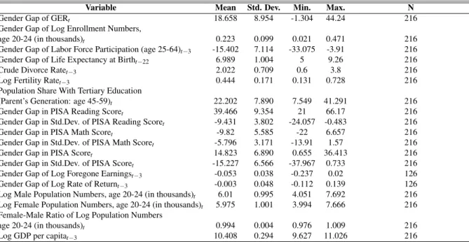
Table 5.1 shows the summary statistics for the baseline sample (2003-2014, 18 countries). Variables are lagged due to potential endogeneity issues and to make them capture the year in which now-enrolled students made their edu-cational investment decisions (see chapter 6 for a more detailed explanation). Summary statistics for regional country subgroups can be found in table A.3 in the appendix.

The average gender gap of the gross enrollment ratio with 18.6 percentage points is positive and hence in favor of women. A positive average gender gap can also be found for life expectancy at birth and PISA scores: Women, on average, live almost seven years longer than men and score 39.5 points higher in PISA reading exams. The average gender gap of labor force participation, foregone earnings and the "earnings premium" of tertiary education, on the contrary, are still negative and to the detriment of women. Table A.3 in the appendix

1_{Pekkarinen (2012) ﬁnds that in countries where the gender gap in reading was high in favor of women, the}

gender gap in mathematics was close to zero or very low in favor of men.

2_{Nevertheless, in a robustness check we will run a regression also with PISA math scores and the average of}

(37)

22 Chapter 5. Data Sampling and Variable Definition

Table 5.1: Summary Statistics in Levels

Variable Mean Std. Dev. Min. Max. N Gender Gap of GERt 18.658 8.954 -1.304 44.24 216

Gender Gap of Log Enrollment Numbers,

age 20-24 (in thousands)t 0.223 0.099 0.021 0.471 216

Gender Gap of Labor Force Participation (age 25-64)t−3 -15.402 7.114 -33.075 -3.91 216

Gender Gap of Life Expectancy at Birtht−22 6.989 1.004 5 9.26 216

Crude Divorce Ratet−3 2.022 0.709 0.6 3.8 216

Log Fertility Ratet−3 0.444 0.171 0.131 0.728 216

Population Share With Tertiary Education

(Parent’s Generation: age 45-59)t 22.202 7.890 7.549 41.291 216

Gender Gap in PISA Reading Scoret 39.466 9.354 21 66.17 216

Gender Gap in Std.Dev. of PISA Reading Scoret -9.431 3.802 -24.057 -0.483 216

Gender Gap in PISA Math Scoret -9.82 5.585 -22 6.657 216

Gender Gap in Std.Dev. of PISA Math Scoret -5.796 3.171 -13.91 1.57 216

Gender Gap in PISA Scoret 14.823 6.890 0.655 36.413 216

Gender Gap in Std.Dev. of PISA Scoret -15.227 6.566 -37.967 0.733 216

Gender Gap of Log Foregone Earningst−3 -0.053 0.038 -0.237 0.02 126

Gender Gap of Log Rate of Returnt−3 -0.003 0.048 -0.112 0.139 126

Log Male Population Numbers, age 20-24 (in thousands)t 6.01 0.995 4.051 7.692 216

Log Female Population Numbers, age 20-24 (in thousands)t 5.975 1.001 3.994 7.666 216

Female-Male Ratio of Log Population Numbers

age 20-24 (in thousands)t 0.994 0.004 0.976 1.009 216

Log GDP per capitat−3 10.408 0.294 9.627 11.026 216

The gender gap always refers to female-male values. PISA scores refer to the average of math and reading scores when not explicitly called math or reading scores.

shows differences between country subgroups: the average GER gender gap, for example, is highest in Nordic countries and lowest in Western European ones. Similarly, the mean gender gap in PISA reading scores is highest among Nordic and lowest among Western European countries.

Data was collected from different online databases. A table with the source by variable can be found in A.2 in the appendix. Countries were selected based on two criteria: by limiting the country sample to European OECD countries, only relatively homogeneous countries were selected to make sure that all countries experienced a faster increase in female than in male enrollment and a widening of the gender gap in favor of women. Second, some countries had to be dropped from the sample due to lack of data availability. Data availability also determined the time dimension of the sample. The baseline sample therefore covers 18 countries and the period 2003-20143. Another concern with respect to data were missing values. To avoid a high loss of information due to list-wise deletion, we used linear interpolation to deal with missing values. Nevertheless, countries for

3_{Countries included: The Nordic countries Denmark, Finland, Sweden and Norway; the Western European}

countries Belgium, France, the Netherlands, Ireland and Great Britain; the Southern European countries Spain, Greece, Italy and Portugal as well as the Eastern European Countries Czech Republic, Poland, Hungary, Slovenia and Slovakia.

(38)

5.3. Summary Statistics 23

which too many values were missing consecutively or for which data was not available for earlier years could not be added to the sample.

Scatter plots which show correlations between the dependent and the explanatory variables can be found in ﬁgures A.4 - A.12 in the appendix for pooled as well as a country and time demeaned data.

(39)

(40)

25

6 Empirical Analysis

6.1 Methodology

We want to estimate the effect of gender differences in labor market factors, health factors, marriage market factors, household production factors and costs of tertiary education on the gender gap in gross enrollment ratios with the following level-speciﬁcation:

Y_i,t = αi+ β1X1i,t−3+ β2X2i,t−3

| {z }

labor market factors

+ β₃X₃_i,t₋₃ | {z } marriage market factor + β4X4i,t−22 | {z } health factor + β5X5i,t−3+ β6X6i,t−3 | {z } household production factors + β7X7i,t−3+ β8X8i,t−3 | {z } cost factors +δt+ ζi,t+ εi,t (6.1)

Where Y_i,t is the female-male gender gap of gross enrollment ratios in tertiary education. Where X₁_i,t₋₃ is the gender gap in labor force participation rates, X₂_i,t₋₃ is the gender gap in the "earnings premium" to tertiary education (in logs), X₃_i,t₋₃ is the crude divorce rate, X₄_i,t₋₂₂ is the gender gap in life expectancy at birth,

X₅_i,t₋₃ is the fertility rate (in logs), X₆_i,t₋₃ is the populationshare with tertiary degree of the parent’s generation. X₇_i,t₋₃ is the gender gap of foregone earnings (in logs) and X₈_i,t₋₃ is the gender gap in PISA reading scores. In addition,α_iare country ﬁxed effects,δt time ﬁxed effects, and ζi,t is GDP per capita (in logs) as

a country-year effect. X_t₋₃ indicates that variable X is lagged by 3 years or 22 years in case of X_t−22.

(41)

26 Chapter 6. Empirical Analysis

The combination of time-series and cross-section dimensions of our data brings along an important set of advantages over simple cross-section or simple-time series data: First, it increases the number of observations and thereby allows to infer model parameters more accurately due to higher sample variability and more degrees of freedom. Second, it allows to better control for the effects of unobserved heterogeneity (Cameron and Trivedi, 2005). Equation 6.1 can be estimated efﬁciently and consistently using OLS, only if stationarity can be assured and if the covariance of the errors meets the Gauss-Markov assumptions. When this is not the case, OLS estimation reports inaccurate standard errors which cause inefﬁcient and inconsistent estimates (Beck, 2008). Violation of these assumptions can result from the data’s time-series dimension or from its cross-sectional dimension:

Endogeneity

One violation of the Gauss-Markov assumptions are error terms which are correlated with the dependent variable. A possible cause for this violation is endogeneity from reverse causality. If endogeneity is present, estimates are likely to be biased and inconsistent. Variables such as fertility and labor force participation, for instance, can suffer from reverse causality with respect to enrollment in tertiary education. We expect fertility rates at time t to inﬂuence enrollment in tertiary education at time t, however, also enrollment at time t is expected to affect fertility rates at time t. The same line of argumentation can be made for other explanatory variables such as labor force participation rates. A common and easy-to-implement approach to address reverse causality is the use of lagged explanatory variables. While for instance, enrollment in t affects fertility rates in t and t+x, enrollment in t does not affect fertility rates in t-x. In this dissertation, most explanatory variables are therefore lagged by three years. The number of three was chosen to simultaneously make the variables capture values of approximately the year in which the now enrolled students had made their investment decisions.