Market Illiquidity and the Bid-Ask Spread of
Derivatives
João Amaro de Matos
1and Paula Antão
Faculdade de Economia
Universidade Nova de Lisboa
Rua Marquês de Fronteira 20
1099-038 Lisbon, Portugal
March 27, 2000
1Corresponding author’s contact: [email protected]. The authors would like to
thank the comments of Bernard Dumas, Marcelo Fernandes, José Miguel Gaspar, Pekka Hietala and Pierre Hillion.
Abstract
This paper analyzes the impact of illiquidity of a stock on the pricing of derivatives. In particular, it is shown how illiquidity generates a bid-ask spread in an option on this stock, even in the absence of other imperfec-tions, such as transaction costs and asymmetry of information. Moreover, the spread is shown to be asymmetric with respect to the option price under perfect liquidity. This fact explains the appearance of a smile e¤ect when the implied volatility is estimated from the mid-quote.
1 Introduction
Many studies suggest that bid-ask spreads in …nancial markets are the result of some market imperfections. Examples of such imperfections are inventory-carrying costs as in Amihud and Mendelson (1980) and Stoll (1978), transac-tion costs as in Boyle and Vorst (1992) and asymmetric informatransac-tion costs as in Glosten and Milgrom (1985) and Easley and O’Hara (1987). In this work a model is presented, in which the bid-ask spread is generatedonly as a con-sequence of illiquidity in the stock market. This modelization of the bid-ask spread comes very much in the spirit of the recent paper of Cho and En-gle (1999), who empirically explain the spreads in a perfect derivative hedge world by the illiquidity of an underlying market, rather than by the usual imperfections. Our paper fully formalizes some of their empirical …ndings. Moreover, the power of the model becomes evident in an explanation (at least qualitative) of the smile e¤ect in very simple terms, reinforcing the idea in Bossaerts and Hillion (1997) that these type of e¤ects may be explained in terms of constraints on the frequency of hedge portfolio rebalancing.
Most option pricing models assume perfect frictionless markets. The value of an option is computed using a portfolio on the underlying risky asset and risk-free bonds that replicates the payo¤s of the option. As both the risky asset and the risk-free bonds are priced in the market, it is possible to compute the theoretical value for the option that rules out any arbitrage opportunity. It is also assumed that the replicating portfolio is adjusted at each point in time in order to replicate the value of the option. This possibility of continuous rebalancing is one of the assumptions taken in the Black and Scholes (1973) valuation formula.
However, in real-world …nancial markets, there are imperfections and it is not always possible to accept the Black and Scholes valuation model. One of these imperfections is related to the continuous rebalancing hypothesis. This hypothesis has been dropped in several studies, mainly because of the existence of transaction costs1. In the presence of transaction costs, the Black
and Scholes arbitrage argument can no longer be used because the replicating strategy would be extremely costly. To take into account the impact of this imperfection on the price, most authors assume that trading takes place only between discrete time intervals. Other reasons can lead to the acceptance of discrete-time rebalancing, namely the fact that markets close every day.
This paper assumes a completely di¤erent reason for discrete time re-balancing of portfolios. Speci…cally, it is assumed that portfolios cannot be
rebalanced on consecutive dates, even in a discrete-time setting, because mar-kets are illiquid. Illiquidity has become a very important matter for those acting in …nancial markets, specially after so many crises in emerging mar-kets, such as the one that occurred in mid-1998 after the Russian government defaulted Russian Treasury-Bills. The point is that the e¤ective value of a portfolio depends on the degree of market’s liquidity. In fact, to liquidate an investor’s position in a situation where assets are illiquid, it may be di¢cult to obtain the true value of the assets involved. In some cases it may be necessary to wait a certain period of time before transaction prices are well de…ned.
A measure of market illiquidity will therefore be related to the time in-terval between portfolio rebalancing, and will have consequences in the way derivatives are priced. As opposed to the papers dealing with transaction costs, our work implies a pricing framework equivalent to that of incomplete markets, in the spirit of the papers by El Karoui and Quenez (1991,1995) and Edirisinghe, Naik and Uppal (1993). Notice that in our context market incompleteness derives from the fact that markets are illiquid. In the usual incomplete markets framework rebalancing is possible at every point in time. In our framework, this is not so.
As in Leland (1985) and Boyle and Vorst (1992), the possibility of trad-ing in the underlytrad-ing asset is exogenously restrained to some points in time, giving rise to a so-calledtime-based hedging strategy. Likewise, it will be as-sumed in this paper that trading in the underlying asset can be done only in pre-determined …xed points in time, re‡ecting the fact that markets are illiq-uid. A di¤erent approach by Bensaid, Lesne, Pagès and Sheinkman (1992), Edirisinghe, Naik and Uppal (1993) and Naik and Uppal (1993), among oth-ers, consider the hedging dates as a variable to be endogenously solved by an optimization model. The resulting optimal hedging strategy, the so-called move-based hedging strategy, leads to the conclusion that in the presence of transaction costs it may not be optimal to revise the hedge portfolio at every point in time. Although a time-based trading strategy may not be optimal, it may be “justi…ed mainly by economical and institutional reasons” as argued by Toft (1996).
The Black-Scholes assumption on the possibility of continuous rebalanc-ing is dropped again in the recent work of Kamal and Derman (1999). These authors assume that options are replicated in line with the Black-Scholes strategy, but only at certain points in time, leading to a replicating error. The approach to the problem is quite di¤erent in this paper, since there
will be no replicating error. Instead, we do the following: consider a market-maker who sells and buys options. When transacting a derivative instrument, the replicating portfolio of this intermediary is rebalanced whenever possible in time, in such a way as to guarantee that its future value always covers the future value of the transacted option. The hedging portfolio built in this way is perfectly analogous to the superreplicating portfolio in El Karoui and Quenez (1991,1995) and Karatzas and Kou (1996) in the framework of in-complete markets in continuous time. Then, although the adjustment of the replicating portfolio can take place only in discrete time, the options’ dealers will be fully hedged against the exercise of the options. As stressed by El Karoui and Quenez (1991,1995) and Karatzas and Kou (1996), since markets are incomplete, the hedging of the market-maker is di¤erent depending on whether he is in a long or sort position. This results in two di¤erent prices for the option, a bid and an ask price.
The option ask price corresponds to the minimum value of a replicating portfolio for the long position in an option, that is, the minimum price that is asked when an investor wants to buy it. The option bid price corresponds to the maximum value of a replicating portfolio for a short position in the option. As expected, the value of the option in the presence of a liquid stock market is shown to lie between the ask and bid values, when markets are illiquid. Furthermore, as the market becomes more liquid, both bid and ask prices converge to the liquid price. In the continuous-time setting, we conclude that options’ prices are given by the usual Black-Scholes option valuation where the volatility comes adjusted to re‡ect market illiquidity. This is similar to Leland (1985) and Boyle and Vorst (1992) conclusions in the presence of transaction costs. However, their adjusted volatilities become in…nite as the time between rebalancing points goes to zero, making it di¢cult to interpret their formulas in continuous-time.
Krakovsky (1999) de…nes market liquidity of an asset as the sensitivity of the stock’s price to the transaction volume. For a given sensitivity, he also arrives to a liquidity adjusted Black-Scholes equation which is nonlinear in the option’s price. His equation has the disadvantage that can only be solved numerically.
The article is organized as follows. In section 2 the methodology of the paper is illustrated in the simple context of a binomial two-period model. The next section extends this analysis to consider both the e¤ect of longer time-to-maturity and the e¤ect of a higher level of illiquidity in the stock market. The model is developed for the case of continuous time in section
4. Section 5 presents some numerical results on the bid-ask spread and some empirical implications of our results. The main conclusions of the article are presented in the last section.
2 The Bid and Ask Prices in a Two-Period
Model
This section is based on the well-known binomial option pricing model devel-oped by Cox, Ross, Rubinstein (1979). In this model the stock price follows a binomial process over discrete periods. In each period the value of the stock may evolve in two di¤erent ways: it may be multiplied either by a rate U or by a rate D, where U > R > D and R denotes one plus a constant riskless interest rate over each time period.
We begin by considering a European call option with exercise price K and two periods to maturity. In this simpli…ed model there are three relevant dates: t = 0; 1; 2: At t = 0 the option is traded for a value C, and at t = 2 the option matures and its value is given by max(0; S2¡ K), where S2 is the
value of the stock at time t = 2.
The call option will take the following notation at each node: at t = 1, if the stock price is raised by the rate U; the option’s value is denoted by CU:
Otherwise, if the stock price is raised by the rate D; the option’s value at t = 1 will be denoted by CD. Similarly, for t = 2 the possible values for the
option will be denoted by CU U; CU D and CDD: Since t = 2 is the maturity of
the contract it follows that CU U = max [0; U U S¡ K]
CU D = max [0; U DS¡ K]
CDD = max [0; DDS¡ K]
2.1 The Two-Period Liquid Model
If there are no arbitrage opportunities, a call option must be worth the same as the cheapest portfolio that exactly replicates the value of the call at each point in time. Considering a simpli…ed economy with one risky asset (the underlying) and one-period riskless bonds, one such portfolio may be
constructed. At each point in time this portfolio consists of ¢ shares of the stock and an amount B in riskless bonds. As time changes, the portfolio is adjusted to continue replicating the values of the call option. Then, at t = 0; a portfolio of ¢0shares and an amount B0 in the riskless asset is built
such that it replicates the value of the call at t = 1: At t = 1 the portfolio is adjusted to replicate the option at maturity. For longer maturities, this implies that everytime the price changes, there may be transactions in the market of the underlying stock and in the market of bonds to adjust the hedging portfolio.
If there are no arbitrage opportunities, the value of the call option at each point in time and at each possible state of Nature must be the same as the value of this corresponding hedging portfolio, since both the call and the portfolio have exactly the same payo¤s at the next point in time.
For this two period model, it is well known that the value of the call is C = [p2C U U+ 2p(1¡ p)CU D+ (1¡ p)2CDD] =R2 where p = R¡D U¡D and 1 ¡ p = U¡R U¡D.
2.2 Modelling Illiquidity
Although widely discussed, there is no agreement either on how to de…ne liquidity or on how to measure it. Liquidity is often de…ned re‡ecting two dimensions of a transaction. One of these refers to the time taken to convert an asset into cash. Based on this dimension, an asset is liquid if it can be immediately transacted. The other dimension, measures the cost of trading an asset for cash quickly. In this case, an asset is liquid if it can be transacted at a price near the prevailing market price.
Liquidity is usually recognized as an important characteristic of capital markets. It is generally accepted that investors prefer to invest in liquid assets that can be traded quickly, and at a low cost, than to invest in illiquid assets, which must o¤er higher expected returns to attract investors2.
Lippman and McCall (1986) present a measurable de…nition of liquidity based on the length of time that it takes to sell an asset. For these authors, money is by de…nition the most liquid asset and they de…ne other asset’s liquidity as the “optimal expected time to transform the asset into money”. By “optimal” it is meant that sellers only accept o¤ers greater or equal to their reservation price. Only when these o¤ers arrive are transactions made.
In the case of a totally illiquid asset, the expected time to convert it into money is in…nite.
The second perspective of de…ning liquidity suggests another measure that is widely used: the bid-ask spread. The bid and ask prices correspond to the prices quoted by …nancial intermediaries who make up the market in a given asset. The ask (bid) price is the price at which the market maker is willing to sell (buy) the asset and it includes a premium for immediacy selling (buying). In fact, market makers solve the problem of the time gap between public buy and sell orders. When an investor does not want to wait for another trader to take the opposite side of the transaction, this investor must trade with the market maker accepting the price that is quoted. Thus, a natural measure of illiquidity is the di¤erence between the bid and ask prices. In this way, a higher bid-ask spread corresponds to a higher immediacy cost and a less liquid asset.
At this point one may introduce the notion of illiquidity as the lack of liquidity. For this purpose assume that at t = 1 trading in the underlying asset is not possible, or in other words, it is not possible to convert money into the asset, or vice-versa, at t = 1. In this speci…c case, it will take two periods of time to achieve these conversions. This clearly typi…es an illiquid market in the sense de…ned by Lippman and McCall (1986). It can be assumed that the reservation price is such that the investor is not willing to trade in t = 1; preferring to postpone his transactions until the next period. The point is to know how this fact a¤ects the pricing of the option.
The above trading restriction implies that the initial portfolio (¢0; B0)
made at t = 0 will not be adjusted after one period. An investor who buys this portfolio (¢0; B0) and keeps it until maturity is not fully hedged because
this portfolio did not consider the evolution of the stock price until time two3.
On the other hand, another portfolio could have been computed considering the three states of Nature at t = 2. Once again, a portfolio computed as is section 2.1 would not replicate the payo¤s of the call option at maturity since it could have the same payo¤s of the call only in two of the three alternative states of Nature. In conclusion, the usual approach to compute replicating portfolios cannot be applied here since the portfolio would not be a fully replicating one. In fact, the illiquid markets assumption will give rise to two di¤erent prices of the call, a bid and an ask price.
The remainder of this section considers the simple case of a two-period model. In a two period model, market illiquidity means that the underlying stock can be traded only at t = 0 and/or t = 2: In this situation, any hedging
portfolio cannot be adjusted at t = 1 and will be kept from t = 0 until the corresponding option expires at t = 2: In the next section a more general case is considered, where the option maturity is expanded from 2 periods to T periods. In a T period model, market illiquidity will be related to the number of periods between two consecutive transactions of the underlying asset, just as in the 2 period model. In the T period model, however, this number of periods may be greater than 2 and the underlying asset may be transacted at di¤erent points in time, allowing the replicating portfolio to be adjusted at each of those points.
2.2.1 The ask price of a call option
Consider a …nancial institution4 selling a call option while wishing to be
hedged. Today, the objective of the institution is to minimize the cost of replicating the exercise value of the option at maturity. It is expected that the buyer of the call option exercises it, at maturity, whenever the value of the stock is greater then the exercise price. Under the simplifying assumption that the economy is composed of the underlying and a riskless asset, this is equivalent to building a hedging portfolio at time t = 0 in these two assets. The replicating portfolio is built in such a way that at t = 2 its value always exceeds, or equals, the exercise value of the option. In other words, the …nancial institution must be prepared to the exercise of the option. If this happens, the institution will certainly need to hold an instrument that is worth at least as much as the exercise value of the option. The problem of the intermediary is to minimize the cost of this initial portfolio, that is, it must be solved the following optimization problem
min ¢S + B f¢; Bg
subject to the terminal conditions: ¢U U S + BR2 ¸ C U U ¢U DS + BR2 ¸ C U D ¢DDS + BR2 ¸ C DD
where CU U; CUD and CDD have the meanings explained at the beginning
of this section.
It is worth noticing that these terminal restrictions are inequalities. Then, the solution of this problem will clearly be super-replicating, since there
cannot be found a unique solution for (¢; B) satisfying the three conditions in equality. In at least one of the three states of nature, the portfolio will have a strictly higher payo¤ than the exercise value of the option. With a portfolio guaranteeing these restrictions, the institution is simultaneously maximizing its pro…ts while being fully hedged against the exercise of the option.
Proposition 1 Solving this problem leads to the ask price of the call Ca= [¼CU U+ (1¡ ¼)CDD] =R2
where ¼ = R2¡D2
U2¡D2 and 1 ¡ ¼ = U 2¡R2
U2¡D2.
Proof. See the Appendix.
It is also shown in the Appendix that
Proposition 2 Ca ¸ C; that is, the cost of the hedging portfolio is greater
when it cannot be adjusted in every period.
In other words, the …nancial institution has a lower bound on its selling price that is higher than in the case of full liquidity. Also, it is worth noticing that this new hedging portfolio has the following property: in the two extreme states of Nature at maturity it has the same value as the call option; in the intermediate state it is worth more than the call.
2.2.2 The bid price of a call option
On the other hand, the …nancial institution is also concerned about the cost of replicating a long call option on the same underlying asset. The problem now is analogous but quite di¤erent. The …nancial institution buys a call option and, to be hedged, sells a hedging portfolio. This is di¤erent from the previous case since it corresponds to short selling the underlying asset while investing in the riskless asset. At maturity, the institution must buy the shares in the market and it also receives the results from the investment in the riskless asset. At the same time, it owns a call option that will exercise if the payo¤ is positive. To be fully hedged against the probability of exercising the option, it must be imposed that the call option’s payo¤ is at least as much as the value of the portfolio. At the same time, and to maximize its pro…ts, the
…nancial institution searches today for the maximum value of the portfolio that it is selling. This corresponds to the following problem
max ¢S + B f¢; Bg
subject to the terminal conditions: ¢U U S + BR2 C
U U
¢U DS + BR2 C U D
¢DDS + BR2 CDD
where again CU U; CU D and CDD have the meanings explained at the
be-ginning of this section.
Once again, these terminal conditions are inequalities. The replicating portfolio will satisfy the restrictions in equality only for two of the three states of Nature. The solution to this problem has another particularity, it has two di¤erent solutions depending on whether (UD ¡ R2) is positive or
negative5. We then have the following.
Proposition 3 The bid price of the call under the assumption that UD < R2
is Cb = [¼0CU U+ (1¡ ¼0)CU D] =R2 where ¼0 = R2¡UD U (U¡D) and 1 ¡ ¼0 = U2¡R2 U(U¡D).
If UD > R2 the bid price of the call is
Cb = [¼00CU D+ (1¡ ¼00)CDD] =R2
where ¼00 = R2¡D2
D(U¡D) and 1 ¡ ¼00 =
U D¡R2
D(U¡D).
Proof. See the Appendix.
It is also shown in the Appendix that Proposition 4 C ¸ Cb.
This means that, to be hedged, the …nancial institution is willing to pay a smaller amount for a call option than the value obtained under full liquidity. It is important to notice that ¼, ¼0and ¼00 have some special properties.
Given the assumption that U > R > D and the additional restrictions for the bid price, it is easily checked that ¼, ¼0and ¼00are always positive and less
2.2.3 The Put option
The problem can be formulated to a European put option. The ask price is obtained minimizing the actual value of a portfolio of the stock and bonds subject to the restriction that its value at t = 2 always exceeds or equals the exercise value of the put option. The problem is quite similar to the one of the ask price of the call option and its solution gives rise to the following expression for the ask price of a put option (Pa):
Pa= [¼PUU + (1¡ ¼)PDD] =R2
where PU U = max(0; K¡ UUS) and PDD = max(0; K¡ DDS).
In the case of the bid price of the option, the problem to be solved is the maximization of the actual value of a portfolio subject to the restriction that it will always value, at maturity, less than or equal to the exercise value of the put option. Once again there will be two situations:
- if (UD ¡ R2) < 0 the bid price of the put is
Pb = [¼0PUU + (1¡ ¼0)PU D] =R2
where PU D = max(0; K¡ UDS);
- if (UD ¡ R2) > 0 the bid price of the put is
Pb = [¼00PU D + (1¡ ¼00)PDD] =R2
Notice that all these expressions for the put prices are very similar to those corresponding for a call option. For instance, the ask price of a put option is a weighted average of its extreme values at the maturity, weighted by ¼ and 1 ¡ ¼; exactly the same as the ask price of a call option. A similar conclusion can be taken for the bid prices. It turns out that the put-call parity is still valid for options on the same stock, with the same exercise price and maturity. From the ask price of a call option, one would obtain the ask price of a put option; from each of the bid prices of the call option, one would get the respective put price.
3 The Bid and Ask Prices in the General
Dis-crete Case
These results can be expanded in two related directions. The …rst one consists in expanding the time to maturity of a call option for T . In this case, it is
necessary to generalize the number of upward movements of the stock price, denoted by j. The second expansion is to consider di¤erent levels of illiquidity in the stock market. In this model, the level of illiquidity is related to the number of periods between two consecutive transactions which will be given by n: In the previous section, for instance, an illiquid market with T = n = 2 was analyzed. In that case there was no opportunity to rebalance the hedging portfolio. But, in the general case where T > n; the initial hedging portfolio will be rebalanced whenever it is possible to trade in the stock market. In the presence of a liquid market, n is equal to one meaning that the hedging portfolio is rebalanced every period.
As in the previous section, the problem is …rst characterized for the ask price. This price is the lowest one for which a …nancial institution would be willing to sell the call option. By de…nition, it is given by the value of the cheapest hedging portfolio composed of ¢ shares and a loan of B; made at t = 0; which will be rebalanced in a way to insure that, at maturity, the seller of the option will have a payo¤ equal or greater to its exercise value: This portfolio will not be rebalanced every period because of stock market illiquidity but it is not static. In fact, it will be rebalanced every n periods, that is, it will be rebalanced at times t = n; 2n; 3n; :::T ¡ n: The problem to be solved in the beginning of each rebalancing period is therefore
min ¢tSt+ Bt
f¢t; Btg
subject to the conditions:
¢tUjDn¡jSt+ BtRn¸ Ct+n;j for j = 0; :::; n and t = 0; n; :::T ¡ n;
(1) where Ct;j is the value of the option at time t; the price of the underlying
stock having increased j times in the last n periods. In particular, CT;j =
max(0; UjDn¡jS
T¡n¡ K):
The problem is basically the same as in the two-period model. The main di¤erence is that the number of restrictions is generalized to be n + 1: It is shown in the appendix that the rebalancing portfolio (¢a;t; Ba;t) is now given
by ¢a;t = Ct+n;nSt(Un¡C¡Dt+n;0n) Ba;t = U nC t+n;0¡DnCt+n;n Rn(Un¡Dn)
It means that, at time t = 0; a portfolio (¢a;0; Ba;0) is constructed
satis-fying restriction (1). By assumption, it is not possible to trade in the stock market after t = 0 and before t = n. Then, the hedging portfolio will be adjusted, for the …rst time, only at t = n: This procedure will be repeated at times t = 2n; 3n; ::: until t = T ¡ n; which is the last rebalancing period before maturity:
The solution to the problem solved in each n-period leads to the following expression of the ask price at time t = 0; n; 2n; :::; T ¡ n of the call as a function of n : Lemma 5 Ca;t = 1 Rn[¼Ct+n;n+ (1¡ ¼)Ct+n;0] (2) where ¼ = Rn¡Dn Un¡Dn; and 1¡ ¼ = U n¡Rn Un¡Dn:
Proof. See the Appendix.
Considering T the maturity of the option6, the general formula for the
ask value of a call option at time t = 0 as a function of payo¤s at maturity is given by Proposition 6 Ca = 1 RT T =n X j=0 µ T =n j ¶ ¼j(1¡ ¼)T =n¡j(UnjDT¡njS¡ K)+ (3) where ¡T =n j ¢ = j!(T =n¡j)!(T=n)!
Proof. Follows working backwards the result of the lemma above. Similarly, the bid price is characterized as the maximum value that the …nancial institution would be willing to pay for a call option. In this case, the problem in each rebalancing period may be stated as constructing a portfolio of ¢ shares and cash B such that
max ¢tSt+ Bt
f¢t; Btg
¢tUjDn¡jSt+ BtRn Ct+n;j for j = 0; :::; n and t = 0; n; :::T ¡ n;
where, as before, Ct;j is the value of the option at time t; the price of the
underlying stock having increased j times in the last n periods.
Once again, the hedging portfolio constructed at t = 0 will be adjusted at times t = n; 2n; 3n; :::T ¡n. This strategy ensures the intermediary a hedged position.
As in the previous section, the computation of the bid price is not straight-forward. It depends on the relation between Rn and the value of the asset
at each rebalancing point in time. Let i be de…ned as the integer satisfying Un¡(i+1)Di+1< Rn < Un¡iDi; and 0 i n¡1: It is shown in the appendix
that the hedging portfolio (¢b;t; Bb;t) is now given by
¢b;t=
Ct+n;n¡i¡Ct+n;n¡(i+1)
St(Un¡iDi¡Un¡(i+1)Di+1)
Bb;t=
Un¡iDiC
t+n;n¡(i+1)¡Un¡(i+1)Di+1Ct+n;n¡i
Rn(Un¡iDi¡Un¡(i+1)Di+1)
Then, the bid price of the call option, at each rebalancing period is given by Lemma 7 Cb;t = 1 Rn[¼ 0C t+n;n¡i+ (1¡ ¼0)Ct+n;n¡i¡1]
where ¼0 = Rn¡Un¡(i+1)Di+1
Un¡iDi¡Un¡(i+1)Di+1; and 1¡ ¼0 =
Un¡iDi¡Rn
Un¡iDi¡Un¡(i+1)Di+1:
Proof. See the Appendix.
Once again taking T as the maturity of the option, the general formula for the bid price at time t = 0 as a function of of payo¤s at maturity is given by Proposition 8 Cb = 1 RT T =n X j=0 µ T =n j ¶ ¼0j(1¡ ¼0)T =n¡j(Uj+T¡T=n(1+i)DT =n(1+i)¡jS¡ K)+ (4)
where ¼0 = Rn¡Un¡(i+1)Di+1
Un¡iDi¡Un¡(i+1)Di+1; (1¡ ¼0) =
Un¡iDi¡Rn
Proof. Follows working backwards the result of the lemma above
When the stock market is liquid, n is equal to one and both the bid and ask prices reduce to the expression of the usual binomial model.
As in the simple two-period model, the put-call parity is still valid. Then, the ask price of a put option can be easily derived from the ask price of a call option and, for each i; the put-call parity can also be used to get the bid price of a put option.
4 Continuous Time
The simple binomial context may be used to derive a continuous time valu-ation equvalu-ation. Suppose that each original time period is divided into 1=h smaller periods and that one takes the limit h ! 0: As in Cox, Ross, Ru-binstein (1979) the variables R; U and D must be adjusted consistently to these new time intervals, preserving average rates of increase and average variance per unit time. This is well known to be satis…ed by the rates Uh = e¾ p h; D h = e¡¾ p h and R
h = Rh per time interval h.
This section will develop the partial di¤erential equations for both ask and bid prices in di¤erent illiquidity contexts. It starts assuming the framework considered until now, namely that between two consecutive transactions there are n time units where the underlying asset cannot be transacted. Being n an integer, it follows that there is a lower bound in the possible bid-ask spreads of option prices, which is far too large compared to the observed values in the market. In the second part of this section our results are generalized to a more ‡exible setting in which after each n-period of non-transaction, the underlying asset may be transacted for m consecutive points in time. This allows for less illiquid situations than the former setting. We refer to Section 5.2.3 for a discussion of the empirical relevance of such extension.
4.1 The PDE for the Ask and Bid Prices
Equation (2) relating the ask value of the call at the beginning of a period and its two possible values after n periods was obtained in the section above. That expression may be rewritten as
Rn¡Dn
Un¡DnCn+ U n¡Rn
where Cj is the value of the option if the price of the underlying stock
increased j times.
Choosing Rh; Uh and Dh in the way just described, and substituting them
in the above expression, it follows that h elog Rhn¡e¡n¾ph en¾ph¡e¡n¾ph i C(en¾phS; ¿ ¡ nh)+ h en¾ph¡elog Rhn en¾ph¡e¡n¾ph i C(e¡n¾phS; ¿ ¡ nh) ¡ RhnC a(S; ¿ ) = 0;
where ¿ denotes the time to maturity.
Expanding the function C around (S; ¿) and then each exponential around h = 0, in the limit when h ! 0 the equation above becomes the Partial Di¤erential Equation 1 2 @2C @S2n¾ 2S2+ @C @SS(log R)¡ C(log R) ¡ @C @¿ = 0 (5) This is simply the Black-Scholes Partial Di¤erential Equation changed by the fact that the volatility is multiplied by pn:
The same procedure as above7 is applied to the equation of the bid price
of the call derived in section 3 which can be rewritten as.
Rn¡Un¡1¡iDi+1
Un¡iDi¡Un¡1¡iDi+1Cn¡i+ U
n¡iDi¡Rn
Un¡iDi¡Un¡1¡iDi+1Cn¡1¡i ¡ CbRn= 0
Substituting all terms and restricting the value of i = n 2 ¡ 1 2; we obtain elog Rhn¡e¡¾ph e¾ph¡e¡¾ph C(e ¾phS; ¿ ¡ nh)+ e¾ph¡elog Rhn e¾ph¡e¡¾ph C(e¡¾ p hS; ¿ ¡ nh) ¡ RhnC b(S; ¿ ) = 0
Expanding the function C around (S; ¿) and then each exponential around h = 0, in the limit when h ! 0 the equation above becomes the Partial Di¤erential Equation 1 2 @2C @S2 ¾2 nS 2+ @C @SS(log R)¡ C(log R) ¡ @C @¿ = 0 (6)
which is, once again, the Black-Scholes Partial Di¤erential Equation where the volatility is now divided by pn:
Notice that, as in the discrete case, the put-call parity remains valid. This simpli…es the derivation of put option prices since they can be obtained using the call prices.
4.2 The PDE for the Ask and Bid Prices in an
Arbi-trarily Illiquid Market
The illiquidity setting described until now is rather strong in the sense that there are many more periods without transactions than periods where is possible to transact the underlying asset. Consider now the more general case where the underlying asset can be transacted at m consecutive points in time, m > 1, and then one must wait n time periods to be able to transact again the underlying asset. Under this notation, the former case is the one where m = 1. In this more general case, the partial di¤erential equations for the ask and bid prices can also be obtained. In particular,
Proposition 9 The partial di¤erential equations for the ask price is 1 2 @2C @S2 n2+ (m¡ 1) m + n¡ 1 ¾ 2S2+@C @SS(log R)¡ C(log R) ¡ @C @¿ = 0: (7) Proof. See the Appendix.
Notice that the only term a¤ected by the illiquidity parameters n and m is the second derivative of C with respect to S: In other words, it is the term multiplied by the volatility, thus allowing the interpretation of the impact of illiquidity as an adjustment of the implied volatility of the returns on the underlying stock. The partial di¤erential equation of the bid price (equation (6)) can also be generalised to consider the less illiquid stock market. Once again, the only di¤erence is in the term multiplying @2C
@S2; and an identical
interpretation follows.
Proposition 10 The partial di¤erential equation satis…ed by the bid price is 1 2 @2C @S2 m m + n¡ 1¾ 2S2+ @C @SS(log R)¡ C(log R) ¡ @C @¿ = 0 (8)
Proof. See the Appendix.
It is worth notice that both expressions resume to equations (5) and (6) when m = 1 and to the usual Black-Scholes when n = 1: One may also notice that since the terms multiplying @2C
@S2 are di¤erent in the two partial
di¤erential equations above, the liquid price resulting with m = 1 and n = 1 is not the mean average of the ask and bid prices. This fact will have severe empirical implications, as discussed below.
5 Empirical Implications
It was shown in the previous sections that in the presence of an illiquid market one arrives at an ask (bid) price for an option which is always greater (lower) than the value obtained in the presence of a liquid stock market. This section will implement these results in three ways. First, using the discrete-time results, some values are computed for the bid and ask prices of a European call option, for a given range of parameter values. In this way it will be possible to compare our results with previous works. Next, an explanation for the usual smile e¤ect is advanced. Finally, the model is applied to some options traded in the market and some implied measures of illiquidity are obtained.
5.1 The discrete-time setting
All the simulations assume the current price of the risky asset to be equal to 100, the time to maturity equal to 1 year and a 10% annual risk-free interest rate. The …rst case analyzed assumes the annual standard deviation of the return on the risky asset to be equal to 20%. These parameter values are the same as in Leland (1985) and Boyle and Vorst (1992) in order to facilitate comparison8. The sensitivity of all call prices to the exercise price and the
level of illiquidity of the stock market is studied. Here, the level of illiquidity is related to the number of periods between two consecutive transactions, denoted by n; and it is assumed to be constant during the entire life of the derivative.
Table 1 presents the values of a European call option for di¤erent exercise prices when the number of periods that one must wait to trade the stock is …xed at n = 3. The …rst column corresponds to the length of time of the subperiods in which the year is divided. The liquid price is computed
assuming that the hedging portfolio is rebalanced on all of these dates. The bid and ask prices are computed assuming that along the T periods there were 2 points in time when it was impossible to trade in the stock market. In all other points it was possible to trade meaning that, for instance, when T = 15 the number of m is 13: The liquid price is obtained with the usual binomial model, but it also corresponds to take n = 1 in either of equations (3) or (4). As expected, all prices decrease with the exercise price. Also, the spread decreases with the number of periods in which the year is divided, keeping …xed the number of periods with no trading. The bid-ask spread is non-monotonic, reaching the highest value when the current stock price is equal to the discounted exercise price9.
Table 2 provides the same information as Table 1 for the case where the number of periods between transactions increases to …ve. As expected, both the bid and ask prices are further away from the liquid price, causing the bid-ask spread to be higher. The point here is that the hedging cost increases with the illiquidity of the stock market. One can also repeat this study for a lower volatility of the underlying asset. In that case, all call prices are lower, but the e¤ect is larger for the ask price. This implies a narrower bid-ask spread.
5.2 The continuous-time setting
5.2.1 The spread
In the former subsection, the spread was obtained for some numerical ex-amples in the discrete-time setting. Here, use of the two Partial Di¤erential Equations for the ask and bid prices leads to the immediate computation of the spread, now in the context of continuous time.
Figure 1 represents the bid-ask spread obtained from our model for the following values ¾ = 0:15; ¿ = 0:25; r = 0:02; n = 3; m = 20; S = 50 and K = 47; 48; :::54; 55:
Notice that the basic features of the spread remain true. The bid-ask spread is non-monotonic, reaching the highest value when the current stock price is equal to the discounted exercise price, where now the discount term is a function of r; ¾2; ¿ ; m and n:
5.2.2 The smile e¤ect
The Black-Scholes pricing model assumes a constant volatility of the un-derlying asset return. However, empirical studies obtain a quite di¤erent result, namelly these studies show that there is a curious relation between the volatility of the underlying asset and the exercise price of the option. What is observed is that out-of-the-money and in-the-money options tend to have a higher implied volatility than at-the-money options. This is called the smile volatility10.
These type of empirical studies are possible because the volatility is the only parameter of the Black-Scholes pricing model that is not observable. Then, using observed market option prices it is possible to compute the implied volatility of the underlying asset return. In this situation, since there is a bid and an ask price for the option, it is usual to employ the mid-quote price between these values.
These results show that the constant volatility assumption is a strong one. However, it is not easy to implement an option pricing model with the nonconstant volatility assumption. For instance, the valuation of an op-tion when the volatility is stochastic employs other parameters which would be di¢cult to estimate. If, on the other hand, one accepts a deterministic volatility function of asset price and/or time11, it would be possible to value
an option based on the Black-Scholes partial di¤erential equation. Dumas, Fleming and Whaley (1998) examined the performance of a model with a deterministic volatility function using S&P options from 1988 to 1993. They found that using this model is no better than using an adjusted volatility version of the Black-Scholes model concluding that “simpler is better”.
According to our model, the mid-quote price between the bid and ask prices is not the liquid price, that is, this is not the price that would prevail in the presence of a liquid market. In fact, the mid-quote price is sistemat-ically above the liquid price. If computed from the liquid price, the implied volatility would be constant by construction. Using the mid-quote price, the smile e¤ect shows up.
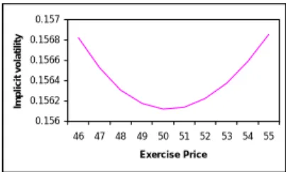
Figure 2 shows the smile e¤ect obtained with a simple simulation of our model. After computing the bid and ask prices of a call option, the mean of these prices was used to get the implied volatility of the underlying asset. It clearly shows that although the bid and ask prices of the option were computed assuming constant volatility, the implied volatility derived from the mid-quote of these prices re‡ects a smile e¤ect12.
It would be interesting to show that, in general, the smile e¤ect results from using the mid-quote of this model. To accomplish that objective, one should be able to prove that d2¾¤
dK2 > 0; for all K; where ¾¤ is the implied
volatility of the underlying asset. Unfortunately, the expression for d2¾¤ dK2 is
so complex that no general conclusion about its sign can be reached beyond the type of simulations performed above.
5.2.3 Market liquidity, implied volatilities and transaction vol-umes
At this point, the model is able to provide a measure of an asset’s illiquidity given the observed values in the market. Given the ask and bid prices of call options written on that asset, one is able to evaluate the implied volatilities, ® and ¯ respectively, using the Black-Scholes formula. According to our model, the implied volatilities are distinct functions of n and m: Therefore, the di¤erences in the implied volatilities obtained from the ask and bid prices, re‡ect a particular choice of n and m: By the fact that we are able to relate the bid-ask spread with the frequency of transactions in the underlying assets, our resulting measure of liquidity is compatible with both the de…nition of Lippman and McCall (1986) and the one based on the bid-ask spread.
From equations (7) and (8) it follows that ® = ¾2 n2+(m¡1)
m+n¡1 and ¯ =
¾2 m
m+n¡1;where ¾2 is the true variance of the returns of the underlying asset.
We notice that ® > ¯ and
®
¯ = 1 + n2¡1
m :
Of course in the perfectly liquid case, n = 1 and ® = ¯: Therefore, one may see the term
¸ = n2m¡1
as a measure of the degree of illiquidity of the market of the underlying asset. It follows that in a perfectly liquid market ¸ = 0 and the value of ¸ increases as the di¤erence between the implied volatilities increases. Notice that the possible values of illiquidity resulting from the model up to section 4.1 were restricted to the values n2 ¡ 1 for n 2 N: In particular, the ratio
of implied volatilities ®=¯ would be restricted to the values n2 for n 2 N:
Introducing the parameter m allows for a much more realistic reading of the empirical results.
In fact, for any observed ® and ¯ it is always possible to …nd integers n and m such that ®=¯ ¡ 1 is suitably approximated by ¸: To see that, de…ne
kxk = inf fk 2 N j k ¸ xg : It then follows
Proposition 11 Given arbitrary positive "; the choice of n = inf 8 < :k 2 N j k2¡1 ®=¯¡1 ° ° °®=¯k2¡1¡1 ° ° ° ¸ 1 ¡ " ¸ 9 = ; and m =°°° n2¡1 ®=¯¡1 ° ° ° ; leads to ®¯ ¡ (1 + ¸) ":
Proof. Notice that ® ¯ ¡ (1 + ¸) = ( ® ¯ ¡ 1)(1 ¡ ¸ ®=¯¡ 1) = ( ® ¯ ¡ 1)(1 ¡ n2¡ 1 ®=¯¡ 1 1 m) (® ¯ ¡ 1)(1 ¡ 1 + " ¸) = ";
where the inequality follows from the de…nition of n; and the claim is proved.
Notice that an error " = 0 is possible only when one can …nd an integer n such that n2¡1
®=¯¡1 is also an integer. On the other hand, since " is an arbitrary
positive number, it follows that there is an increasing subsequence of integers ni; i = 1; 2; :::; such that the error in approaching ®=¯ converges to zero.
A simple and merely indicative study was done with market prices of Monday, 29th November, 1999, from the MEFF (the o¢cial options and
futures market of Spain). The data consists in call options maturing in December 1999, with several exercise prices, and on the following underlying assets: Acerinox, Acesa, BSCH, Endesa and Repsol.
Table 3 presents the values obtained for ®=¯ ¡ 1 using our model, the corresponding values of n, m and ¸ for an error of 0.001 and …nally, the volume of transactions, in thousand euros, of the underlying asset realized on the previous day, that is, 26th November, 1999. Notice that by choosing
the error as 0.001, the values obtained for ¸ coincide with ®=¯ ¡ 1: Also notice that in the case of Acesa, there is the remarkable situation where
n2¡1
®=¯¡1 is an integer with n = 16 and ®=¯ ¡ 1 = 0:600. Therefore, the error in
approximating the value ®=¯ ¡ 1 extracted from data is zero. As expected, there is a negative relation between the illiquidity measure and the volume of transactions, i.e., the measure of market illiquidity increases as the volume of transactions decreases.
6 Conclusions
This paper analyzes the impact of stock market illiquidity on option pricing. Illiquidity of the stock market imposes restrictions on the construction of a hedging portfolio since it is not possible to continuously rebalance it. In this sense, there would be a replicating error if the Black-Scholes strategy were adopted. In this article, another strategy is developed for constructing the rebalancing portfolio that will be superreplicating in the sense used by El Karoui and Quenez (1991,1995). This fully-hedging strategy results in a bid-ask spread in the price of call and put options.
One of the most interesting conclusions is that the liquid price is not in the middle of the bid-ask spread. Therefore, calculations of the implied volatility using the mid-quote will lead to a mistake. This procedure is very common not only in markets but also in empirical papers. The nature of the error incurred has been shown to be compatible with the presence of the smile structure for the implied volatilities.
The framework of this article is related to that of incomplete markets since a superreplicating strategy is developed. But, as opposed to the traditional papers about incomplete markets, we assume that the incompleteness in our case is generated by the impossibility of trading, at certain dates, in complete markets. In other words, our incompleteness is generated by market illiquidity. In a qualitative way, our main results are expressed in equations (7) and (8). As expected, when n = 1 we recover the traditional Black and Scholes formulas. Notice however that when n > 1 our modi…ed Black and Scholes formula for the ask price works as if the variance of the underlying asset had been increased, whereas in the case of the bid price, the Black and Scholes formula works as if the variance of the underlying asset had been decreased. An analogous scaling is found in the literature dealing with transaction costs.
This analysis could be extended to a consideration of American options. In such a case the optimal exercising strategy of the owner of such an
op-tion should be incorporated in the model . Another extension of this work would be to consider a bid-ask spread in the underlying asset. In that case the superreplicating strategy should be adjusted to consider di¤erent buying and selling prices of the shares used to replicate the option. Our intuition is that the option bid-ask spread would be wider were this imperfection to be introduced into the model. In their recent empirical work, Cho and Engle (1999) con…rm our intuition showing that option market spreads are posi-tively related to spreads in the underlying market.
A Appendix
A.1 The Two Period Model
A.1.1 Proof of Proposition 1
The problem is given by min ¢S+B; choosing f¢; Bg subject to the terminal conditions: ¢U2S + BR2 ¸ C U U ¢U DS + BR2 ¸ C U D ¢D2S + BR2 ¸ C DD
The solution follows from the Lagrangean: L = ¢S + B + ¸1(CU U ¡ ¢U2S¡ BR2)
+¸2(CU D¡ ¢UDS ¡ BR2)
+¸3(CDD¡ ¢D2S¡ BR2)
Alternatively, the problem can be solved following Karatzas and Shreve (1998, chapter 5). To value a contingent claim in an incomplete market these authors introduce the notion of auxiliary complete markets. In our case, each auxiliary market is characterized by only two active restrictions out of the three given above. Thus, there are three auxiliary complete markets in this problem. Each auxiliary market must satisfy the illiquidity restriction that no trade is possible at t = 1 and the additional restriction that the terminal wealth always exceeds or equals the payo¤ of the call option at maturity. It then follows that the value of the call option in the constrained market is given by the supremum of all call option prices resulting from the auxiliary (complete) markets.
In this two period model it can be checked that only the auxiliary market resulting from ¸1 > 0; ¸2 = 0 and ¸3 > 0 satis…es the wealth restriction.
The solution to the problem leads to a portfolio with ¢ = CU U¡CDD
S(U2¡D2) and
B = U2CDD¡D2CU U
R2(U2¡D2) : The result follows.
A.1.2 Proof of Proposition 2
From the proof of Proposition 1, notice that Ca¡ C = R22p(1¡ p)
£DCU U+U CDD
U +D ¡ CU D
The proof depends on the way the value of the exercise price K a¤ects the payo¤ at maturity. Then simple substitution of the payo¤s CU U; CDD
and CU D leads to the following situations:
D2S ¸ K ) C a¡ C = 0 U DS > K ¸ D2S ) C a¡ C = R22p(1¡ p) £ ¡ U U +D(D2S¡ K) ¤ ¸ 0 U2S > K ¸ UDS ) C a¡ C = R22p(1¡ p) £ D U +DCUU ¤ > 0; thus proving that in every possible case Ca ¸ C:
A.1.3 Proof of Proposition 3
The problem is given by max ¢S+B; choosing f¢; Bg subject to the terminal conditions: ¢U2S + BR2 C U U ¢U DS + BR2 C U D ¢D2S + BR2 C DD
The solution follows from the Lagrangean: L = ¢S + B + ¸1(¢U2S + BR2 ¡ CU U)
+¸2(¢U DS + BR2¡ CU D)
+¸3(¢D2S + BR2¡ CDD)
Once again, the problem is solved following Karatzas and Shreve (1998, chapter 5). In this case, Karatzas and Shreve’s main result is that the value of the call option in the constrained market is given by the in…mum of all call option prices resulting from the auxiliary (complete) markets.
In this two period model there are three auxiliary markets satisfying the illiquidity restriction, but it can be checked that only two of them satisfy the wealth condition, that is, that the value of the portfolio at maturity is always smaller or equal to the payo¤ of the call option. These markets are the ones resulting from ¸1 < 0; ¸2 < 0, ¸3 = 0 and ¸1 = 0; ¸2 < 0, ¸3 < 0:
The value of the call is given by the in…mum of the initial cost (computed at t = 0) of the portfolio that satisfy the wealth restriction in the complete markets. In other words, corresponds to the maximum price obtained in the two auxiliary markets.
When R2 > U D; the problem is solved with ¢ = CU U¡CU D
S(U2¡UD) and B =
U2C
U D¡UDCU U
R2(U2¡UD) : When U D > R2; the problem is solved with the di¤erent
values of ¢ = CU D¡CDD
S(U D¡D2) and B = U DCDD¡D 2C
U D
R2(UD¡D2) : It follows that the bid
A.1.4 Proof of Proposition 4
Consider the two possible ranges for the values of R : For UD < R2; it follows
that
C¡ Cb = R12(1¡p) 2
U [DCU U¡ (U + D)CU D+ U CDD]
This proof depends again on the value of the exercise price. Then, sub-stituting the values of the payo¤s CU U; CU D and CDD;
D2S ¸ K ) C ¡ C b = 0; U DS > K ¸ D2S ) C ¡ C b = R12 (1¡p)2 U [¡U(D 2S¡ K)] ¸ 0; U2S > K ¸ UDS ) C ¡ C b = R22 (1¡p)2 U [DCU U] > 0;
implying that C ¸ Cb for all possible values of K whenever UD < R2:
Now consider the case where UD > R2: Then,
C¡ Cb = R12p 2
D[DCU U¡ (U + D)CU D+ U CDD] ;
and substituting the values of the payo¤s CU U; CU D and CDD; for the
di¤erent values of the exercise price follows that D2S ¸ K ) C ¡ C b = 0; U DS > K ¸ D2S ) C ¡ C b = R12(1¡p) 2 U [¡U(D2S¡ K)] ¸ 0; U2S > K ¸ UDS ) C ¡ C b = R22(1¡p) 2 U [DCU U] > 0:
Hence, C ¸ Cb for all possible values of K and R:
A.2 The Case of n Periods
A.2.1 Proof of Lemma 5
Now the problem is min ¢tSt+ Bt; choosing f¢t; Btg subject to the
condi-tions:
¢tUjDn¡jSt+ BtRn ¸ Ct+n;j for j = 0; :::; n and t = 0; n; :::T ¡ n;
where Ct;j is the value of the option at time t; the price of the underlying
stock having increased j times in the last n periods. The solution follows from the Lagrangean:
Lt= ¢tSt+ Bt+ n
P
j=0
¸t;j(Ct+n;j ¡ ¢tUjDn¡jSt¡ BtRn)
As in the two-period model, the problem can be solved following Karatzas and Shreve (1998). In this case there are n(n + 1)=2 auxiliary markets to
be considered for each point in time where the call option is to be valued. However, only the auxiliary markets resulting from ¸t;0 > 0 and ¸t;n> 0 are
relevant because all others do not satisfy the wealth restriction. The solution of the problem leads to ¢a;t = CSt+n;nt(Un¡C¡Dt+n;0n) and Ba;t =
UnC
t+n;0¡DnCt+n;n
Rn(Un¡Dn) :
The resulting value of the call is thus the one given in the statement of the Proposition.
A.2.2 Proof of Lemma 7
The problem is now max ¢tSt+ Bt; choosingf¢t; Btg subject to the
condi-tions:
¢tUjDn¡jSt+ BtRn Ct+n;j for j = 0; :::; n and t = 0; n; :::T ¡ n;
where Ct;j is the value of the option at time t; the price of the underlying
stock having increased j times in the last n periods. The solution follows from the Lagrangean:
Lt= ¢tSt+ Bt+ n
P
j=0
¸t;j(Ct+n;j ¡ ¢tUjDn¡jSt¡ BtRn)
Following Karatzas and Shreve (1998), one can costruct n(n + 1)=2 aux-iliary markets. However, in this speci…c case, only the auxaux-iliary markets corresponding to two consecutive negative Lagrangean multipliers satisfy the wealth restriction, giving rise to n call prices. As in the two period model, the value of the call is given by the maximum price obtained in the n auxiliary markets. The solution of the problem leads to ¢b;t =
Ct+n;n¡i¡Ct+n;n¡(i+1)
St(Un¡iDi¡Un¡(i+1)Di+1)
and Bb;t =
Un¡iDiC
t+n;n¡(i+1)¡Un¡(i+1)Di+1Ct+n;n¡i
Rn(Un¡iDi¡Un¡(i+1)Di+1) , where i is de…ned as the
in-teger satisfying Un¡(i+1)Di+1 < Rn < Un¡iDi; and 0 i n¡ 1: It results
that the value of the call option is the one given in the statement of the Proposition.
A.3 Continuous Time
A.3.1 Proof of Proposition 9
Let m be the number of initial points in time with transactions, including t = 0: Since n is de…ned as the number of periods one must wait to transact the underlying asset, n ¡ 1 is the number of points in time between two consecutive transactions. Taking p = R¡D
U¡D and ¼ =
Rn¡Dn
1. the term multiplying C is m¡1P j=0 ¡m¡1 j ¢ pj(1¡ p)m¡1¡j ¡ (1 + (m + n ¡ 1)hr) = ¡(m + n ¡ 1)hr;
2. the term multiplying @C @¿ is mP¡1 j=0 ¡m¡1 j ¢ pj(1¡ p)m¡1¡j(¡(m + n ¡ 1)h) = ¡(m + n ¡ 1)h;
3. the term multiplying @C @S¾ p hS is mP¡1 j=0 ¡m¡1 j ¢ pj(1¡ p)m¡1¡j[¼(2j + n + 1¡ m) + (1 ¡ ¼)(2j ¡ n + 1 ¡ m)] = hr ¾ph(m + n¡ 1) and …nally
4. the term multiplying @2C
@S2¾2hS2 is mP¡1 j=0 ¡m¡1 j ¢ pj(1¡ p)m¡1¡j[¼(2j + n + 1¡ m)2+ (1¡ ¼)(2j ¡ n + 1 ¡ m)2] = n2+ m¡ 1:
Then, the partial di¤erential equation can be rewritten as ¡rC ¡ @C @¿ + @C @SSr + @2C @S2¾2S2 n 2+m¡1 m+n¡1 = 0:
A.3.2 Proof of Proposition 10
This proof follows as in the previous case, but now with p = R¡D U¡D and
¼0 = Rn¡D
U¡D : Then,
1. the term multiplying C is
m¡1P j=0 ¡m¡1 j ¢ pj(1¡ p)m¡1¡j ¡ (1 + (m + n ¡ 1)hr) = ¡(m + n ¡ 1)hr;
2. the term multiplying @C @¿ is m¡1P j=0 ¡m¡1 j ¢ pj(1¡ p)m¡1¡j(¡(m + n ¡ 1)h) = ¡(m + n ¡ 1)h;
3. the term multiplying @C @S¾ p hS is mP¡1 j=0 ¡m¡1 j ¢ pj(1¡ p)m¡1¡j[¼0(2j + 2¡ m) + (1 ¡ ¼0)(2j¡ m)] = ¾hrp h(m + n¡ 1) and …nally
4. the term multiplying @2C
@S2¾2hS2 is m¡1P j=0 ¡m¡1 j ¢ pj(1¡ p)m¡1¡j[¼0(2j + 2¡ m)2+ (1¡ ¼0)(2j¡ m)2] = m:
Then, the partial di¤erential equation satis…ed by the call price is given by ¡rC ¡ @C @¿ + @C @SSr + @2C @S2¾2S2m+nm¡1:
Footnotes
1. Leland (1985), Merton (1990), Boyle and Vorst (1992) and Toft (1996), among others, have examined the impact of transaction costs on option val-uation.
2. This topic was discussed by Amihud and Mendelson (1986, 1988, 1991) 3. This is the case presented in Kamal and Derman (1999).
4. It will not be speci…ed which …nancial institution is a market maker since it di¤ers between exchanges.
5. This distinction does not make any sense when UD = 1: In that case, R2 allways exceeds UD as long as the interest rate is strictly positive, what
seems reasonable. However, in discrete-time analysis one does not need to impose UD = 1: This assumption will be valid only in the continuous-time model.
6. In the discrete-time model one must impose a simplifying assumption that T is a multiple of n;but this assumption is no longer needed in the constinuous-time framework of the next section.
7. To choose Rh; Uh and Dh in the way described, some additional
restrictions must be imposed. If Rn¡Un¡1¡iDi+1
Un¡iDi¡Un¡1¡iDi+1 is to be positive then
hnr¡(n¡2¡2i)¾ph must also be positive. This implies that ¡(n¡2¡2i)n > 0. At the same time, if Un¡iDi¡Rn
Un¡iDi¡Un¡1¡iDi+1 > 0; then n¡2in > 0: Both conditions
imply that n
2 ¡ 1 < i < n
2: As i and n are positive integers, it can be
concluded that the only relevant cases occur when n is odd and i = n 2 ¡
1 2:
8. As in their work, Uh = exp(¾
p
h); Dh = 1=Uh and Rh = Rh; where
h is the length of time of a subperiod in which the year is subdivided. In the case of a liquid market, h is also the time interval between rebalancing times.
9. Boyle and Vorst (1992) have a similar result in their work with trans-action costs.
10. In fact, Dumas, Fleming and Whaley (1998) computed S&P option-implied volatilities for a period after the October 1987 crash and obtained the result that instead of a smile what appears is a sneer, that is, the implied volatilities decrease monotonically as the exercise price rises.
11. Rubinstein (1985) and Derman and Kani (1994), among others, de-velop variations of deterministic volatility function models.
12. The values used in the model were: ¾ = 0:15; ¿ = 0:25; r = 0:02; n = 3; m = 20; S = 50 and K = 46; 47; 48; :::54; 55:
References
Amihud, Y. and H. Mendelson, 1980, “Dealership Market: Market-Making with Inventory”, Journal of Financial Economics, 8, 31-53.
Amihud, Y. and H. Mendelson, 1986, “Asset Pricing and the Bid-Ask Spread”, Journal of Financial Economics, 17, 223-249.
Amihud, Y. and H. Mendelson, 1988, “Liquidity and Asset Prices: Financial Management Implications”, Financial Management, Spring.
Amihud, Y and H. Mendelson, 1991, “Liquidity, Asset Prices and Financial Policy”, Financial Analysts Journal, November-December, 56-66.
Bensaid, B., J. Lesne, H. Pagès and J. Scheinkman, 1992, “Derivative Asset Pricing with Transaction Costs”, Mathematical Finance, 2, 63-86.
Black, F. and M. Scholes, 1973, “The Pricing of Options and Corporate Liabilities”, Journal of Political Economy, 3, 637-354.
Bossaerts, P. and P. Hillion, 1997, “Local Parametric Analysis of Hedging in Discrete Time”, Journal of Econometrics, 81, 243-272.
Boyle, P. and T. Vorst, 1992, “Option Replication in Discrete Time with Transactions Costs”, Journal of Finance, 47, 271-293.
Cho, Y. and R. Engle, 1999, “Modeling the Impacts of Market Activity on Bid-Ask Spreads in the Option Market”, discussion paper 99-05, University of California, San Diego.
Cox, J.C., S.A. Ross and M. Rubinstein, 1979, “Option Pricing: A Simpli…ed Approach”, Journal of Financial Economics, 7, 229-263.
Derman, E. and I. Kani, 1994, “Riding on the Smile”, Risk, 7, 32-39.
Dumas, B., J. Fleming and R. Whaley, 1998, “Implied Volatility Functions: Empirical Tests”, Journal of Finance, 53, 2059-2106.
Easley, D. and M. O’Hara, 1987, “Price, Trade Size, and Information in Securities Markets”, Journal of Financial Economics, 19, 69-90.
Edirisinghe, C., V. Naik and R. Uppal, 1993, “Optimal Replication of Op-tions with TransacOp-tions Costs and Trading RestricOp-tions”, Journal of Finan-cial and Quantitative Analysis, 28, 117-138.
El Karoui, N. and M.C. Quenez, 1991, “Programation Dynamique et éval-uation des actifs contingents en marché incomplet”, Comptes Rendues de l’ Academy des Sciences de Paris, Série I, 313, 851-854
El Karoui, N. and M.C. Quenez, 1995, “Dynamic programming and pricing of contingent claims in an incomplete market”,SIAM Journal of Control and Optimization, 33, 29-66.
Glosten, L. and P. Milgrom, 1985, “Bid, Ask and Transaction Prices in a Spe-cialist Market with Heterogeneously Informed Traders”,Journal of Financial Economics, 14, 71-100.
Kamal, M. and E. Derman, 1999, “Correcting Black-Scholes”,Risk, January, 82-85
Karatzas, I. and S. G. Kou, 1996, “On the Pricing of Contingent Claims with Constrained Portfolios”, Annals of Applied Probability, 6, 321-369.
Krakovsky, 1999, “Pricing Liquidity into Derivatives”, Risk, December, 65-67.
Leland, H., 1985, “Option Pricing and Replication with Transactions Costs”, Journal of Finance, 40, 1283-1301.
Lippman, S. A., and J. J. McCall, 1986, “An Operational Measure of Liq-uidity”, American Economic Review, 76, March, 43-55.
Merton, C., 1990, Continuous Time Finance, Basil Blackwell, sec. 14.2. Naik, V. and R. Uppal, 1994, “Leverage Constraints and the Optimal Hedg-ing of Stock and Bond Options”, Journal of Financial and Quantitative Anal-ysis, 29, 199-222.
Stoll, H., 1978, “The Supply of Dealer Services in Securities Markets”, Jour-nal of Finance, 33, 1133-1151.
Toft, K., 1996, “On the Mean-Variance Tradeo¤ in Option Replication with Transaction Costs”,Journal of Financial and Quantitative Analysis, 31, 233-263.
Rubinstein, M., 1985, “Nonparametric Tests of Alternative Option Pricing Models Using all Reported Trades and Quotes on the 30 Most Active CBOE Option Classes from August 23, 1976 through August, 31, 1978”, Journal of Finance, 40, 455-480.
Table 1: Prices of a European Call option when the number of periods be-tween two transactions is three.
Time units Exercise Price Bid Price Liquid Price Ask price Spread (years) K (n = 3) (n = 1) (n = 3) 1/15 80 28.107 27.696 27.569 0.537 90 20.656 19.736 19.436 1.220 100 14.472 13.079 12.603 1.869 110 9.628 8.032 7.463 2.165 120 6.007 4.519 3.967 2.040 1/30 80 27.855 27.660 27.598 0.257 90 20.150 19.703 19.556 0.594 100 13.619 12.924 12.689 0.930 110 8.780 7.982 7.707 1.073 120 5.315 4.568 4.306 1.001 1/45 80 27.806 27.676 27.633 0.172 90 19.978 19.683 19.585 0.393 100 13.477 13.022 12.869 0.608 110 8.467 7.932 7.751 0.716 120 5.062 4.391 4.563 0.499
Table 2: Prices of a European Call option when the number of periods be-tween two transactions is …ve.
Time units Exercise Price Bid Price Liquid Price Ask Price Spread (years) K (n = 5) (n = 1) (n = 5) 1/15 80 29.229 27.696 27.452 1.777 90 22.899 19.736 19.119 3.780 100 17.625 13.079 12.064 5.561 110 13.101 8.032 6.808 6.294 120 9.207 4.519 3.343 5.864 1/30 80 28.348 27.660 27.538 0.810 90 21.220 19.703 19.404 1.816 100 15.225 12.924 12.440 2.785 110 10.586 7.928 7.413 3.173 120 6.991 4.568 4.028 2.963 1/45 80 28.126 27.676 27.592 0.534 90 20.679 19.683 19.486 1.194 100 14.532 13.022 12.710 1.822 110 9.689 7.932 7.560 2.129 120 6.199 4.391 4.212 1.988
Table 3: Market illiquidity measure and transaction volume. ®=¯ n m ¸ transactions (ths euros) Endesa 0.278 4 54 0.278 380 985 BSCH 0.309 8 204 0.309 117 245 Repsol 0.327 7 147 0.327 65 672 Acerinox 0.538 12 266 0.538 3 560 Acesa 0.600 16 425 0.600 2 188
Figure 1: Spread 0 0.05 0.1 0.15 0.2 0.25 0.3 47 48 49 50 51 52 53 54 55 E x e r c i s e P r i c e Spread
Figure 2: The smile e¤ect 0.156 0.1562 0.1564 0.1566 0.1568 0.157 46 47 48 49 50 51 52 53 54 55 Exercise Price Implicit volatility