i
MODELING MALARIA CASES ASSOCIATED WITH ENVIRONMENTAL RISK
FACTORS IN ETHIOPIA USING GEOGRAPHICALLY WEIGHTED REGRESSION
ii
MODELING MALARIA CASES ASSOCIATED WITH
ENVIRONMENTAL RISK FACTORS IN ETHIOPIA USING THE
GEOGRAPHICALLY WEIGHTED REGRESSION MODEL,
2015-2016
Dissertation supervised by
Dr.Jorge Mateu Mahiques,PhD
Professor, Department of Mathematics University of Jaume I
Castellon, Spain
Ana Cristina Costa, PhD
Professor, Nova Information Management School
University of Nova Lisbon, Portugal
Pablo Juan Verdoy, PhD
Professor, Department of Mathematics University of Jaume I
Castellon, Spain
iii DECLARATION OF ORIGINALITY
I declare that the work described in this document is my own and not
from someone else. All the assistance I have received from other people
is duly acknowledged, and all the sources (published or not published)
referenced.
This work has not been previously evaluated or submitted to the
University of Jaume I Castellon, Spain, or elsewhere.
Castellon, 30th Feburaury 2020
iv Acknowledgments
Before and above anything, I want to thank our Lord Jesus Christ, Son of GOD, for his blessing and protection to all of us to live. I want to thank also all consortium of Erasmus Mundus Master's program in Geospatial Technologies for their financial and material support during all period of my study. Grateful acknowledgment expressed to Supervisors: Prof.Dr.Jorge Mateu Mahiques, Universitat Jaume I(UJI), Prof.Dr.Ana Cristina Costa, Universidade NOVA de Lisboa, and Prof.Dr.Pablo Juan Verdoy, Universitat Jaume I(UJI) for their immense support, outstanding guidance, encouragement and helpful comments throughout my thesis work. Finally, but not least, I would like to thank my lovely wife, Workababa Bekele, and beloved daughter Loise Berhanu and son Nethan Berhanu for their patience, inspiration, and understanding during the entire period of my study.
v
MODELING MALARIA CASES ASSOCIATED WITH
ENVIRONMENTAL RISK FACTORS IN ETHIOPIA USING THE
GEOGRAPHICALLY WEIGHTED REGRESSION MODEL,
2015-2016
ABSTRACT
In Ethiopia, still, malaria is killing and affecting a lot of people of any age group somewhere in the country at any time. However, due to limited research, little is known about the spatial patterns and correlated risk factors on the wards scale. In this research, we explored spatial patterns and evaluated related potential environmental risk factors in the distribution of malaria cases in Ethiopia in 2015 and 2016. Hot Spot Analysis (Getis-Ord Gi* statistic) was used to assess the clustering patterns of the disease. The ordinary least square (OLS), geographically weighted regression (GWR), and semiparametric geographically weighted regression (s-GWR) models were compared to describe the spatial association of potential environmental risk factors with malaria cases. Our results revealed a heterogeneous and highly clustered distribution of malaria cases in Ethiopia during the study period. The s-GWR model best explained the spatial correlation of potential risk factors with malaria cases and was used to produce predictive maps. The GWR model revealed that the relationship between malaria cases and elevation, temperature, precipitation, relative humidity, and normalized difference vegetation index (NDVI) varied significantly among the wards. During the study period, the s-GWR model provided a similar conclusion, except in the case of NDVI in 2015, and elevation and temperature in 2016, which were found to have a global relationship with malaria cases. Hence, precipitation and relative humidity exhibited a varying relationship with malaria cases among the wards in both years. This finding could be used in the formulation and execution of evidence-based malaria control and management program to allocate scare resources locally at the wards level. Moreover, these study results provide a scientific basis for malaria researchers in the country.
Keywords: Ethiopia. Geographically weighted regression. Malaria cases. Non-stationary. Spatial heterogeneity. Risk factors
vi
ACRONYMS
AIC – Akaike Information Criterion
AICc – Akaike Information Criterion
EMA - Ethiopian Metrology Agency GDP – Gross Domestic Product
GIS – Geographic Information System GWR – Geographically Weighted Regression IRS – Indoor Residual Spraying
LLIN – Long-Lasting Insecticidal Nets
MODIS – Moderate Resolution Imaging Spectroradiometer NDVI – Normalized Difference Vegetation Index
S-GWR – Semiparametric Geographically Weighted Regression VIF - Variance Inflation Factor
vii
INDEX OF THE TEXT
Acknowledgments ...iv
Abstract ... v
ACRONYMS ...vi
INDEX OF THE TEXT ...vii
INDEX OF TABLES ... viii
INDEX OF FIGURES ...ix
1 Introduction ... 1
1.1 Motivation, rationale and background ... 1
1.2 Aim and objectives ... 1
1.3 Significance of the study ... 2
1.4 Structure of the report ... 2
2 Literature review ... 2
3 Materials and methods ... 4
3.1 Study area and malaria dataset ... 5
3.2 Climate and environmental data ... 7
3.3 Data pre-processing and modeling ... 8
3.3.1 Environmental data ... 10
3.3.2 Data cleaning and normalization ... 12
3.3.3 Spatial analysis of malaria ... 12
3.3.4 Regression analysis ... 12
4 Results ... 17
4.1 The spatial analysis and distribution of malaria Cases ... 17
4.2 Spatial analysis of predictors... 19
4.3 Ordinary Least Squares model ... 22
4.4 Geographically Weighted Regression model ... 22
4.5 Semiparametric Geographically Weighted Regression ... 36
5 Discussion ... 46
6 Conclusion ... 52
References ... 54
7 Appendices ... 62
7.1 Data cleaning R code ... 62
7.2 Scatter plot of log and logit of malaria incidence for all explanatory variables in 2015 and 2016 ... 63
7.3 R code for exploratory analysis to discover if bivariate relationships were linear or not using B-splines ... 66
7.4 Results of (temperature, Precipitation, elevation and Relative humidity) Variogram models used for interpolation of explanatory variables with ordinary kriging... 69
viii
INDEX OF TABLES
Table 1 Software used for analysis ... 5 Table 2: Variables used in the research and their sources ... 8 Table 3: Variogram models used for interpolation of explanatory variables with
ordinary kriging ... 11 Table 4: Summary of OLS Results - Model Variables for 2015 ... 22 Table 5: Summary of OLS Results - Model Variables for 2016 ... 22 Table 6. Summary of the locally varying coefficients of the variables on the GWR
model in 2015. ... 23 Table 7 Summary of the locally varying coefficients of the variables on the GWR
model in 2016. ... 24 Table 8 Comparison of goodness-of-fit results and residual analysis of the GWR and
OLS models ... 36 Table 9 Comparison of GWR and s-GWR models performances based on AICc .... 37 Table 10 Comparison of OLS, GWR and s-GWR models performances based on
goodness-of-fit measures... 37 Table 11 Summary of s-GWR model coefficients in 2015 ... 38 Table 12 Summary of s-GWR model coefficients in 2016 ... 38
ix INDEX OF FIGURES
Figure 1: Map of the study area covering 679 wards (counties) of the entire country, Ethiopia. ... 6 Figure 2: Annual average malaria incidences in each county from 2015 to 2016 ... 6 Figure 3: Flow chart of the research approach... 9 Figure 4: Each explanatory variable mapped 2015(left) and 2016(right) in the study
area. ... 11 Figure 5 Local Moran’s I test maps of malaria cases and corresponding significance
for 2015 (top) and 2016 (bottom). ... 18 Figure 6. Hot-spot (Getis-Ord Gi* statistic) results of malaria cases in 2015 (a) and
2016 (b) ... 19 Figure 7: Distribution of selected explanatory variables with their corresponding
local (1st column) and global Moran’s I tests (2nd column) ... 21 Figure 8. Pseudo t-values for independent variables in 2015 (left) and 2016 (right) 26 Figure 9. GWR local coefficients of the 2015 model (a-e) ... 27 Figure 10.GWR local coefficients of the 2016 model (a-e) ... 28 Figure 11. Observed (a) and GWR estimated (b) malaria incidence in 2015; observed
(c) and GWR estimated (d) malaria incidence in 2016 ... 35 Figure 12.S-GWR Pseudo t-values for independent variables in 2015 with
significance levels ... 39 Figure 13.s-GWR Pseudo t-values for independent variables in 2016 with
significance levels ... 40 Figure 14. s- GWR local coefficients of the 2015 model (a-d) ... 40 Figure 15. s- GWR local coefficients of the 2016 model (a-c) ... 41 Figure 16.Local R2 (a, b), residual distribution (c, d) in the s-GWR-based prediction
model of the malaria case in 2015 and 2016 ... 48 Figure 17 scatter plot of log and logit of malaria incidence for all explanatory
1
1 INTRODUCTION
1.1 Motivation, rationale and background
In Ethiopia, still, malaria is killing and affecting a lot of people of any age group somewhere in the country at any time. Furthermore, there are a large number of inpatient and outpatient due to malaria case in Ethiopia (Alemu et al. 2011); it is a significant loss in terms of life and money for the country. Therefore, researching modeling malaria cases associated with environmental risk factors in of Ethiopia is very relevant. In Indonesia, (Hasyim et al. 2018) conducted a similar study. In their research, they didn’t include climate factors data for their research data analysis, and they put that as a limitation of their research. Thus this research will try to solve that limitation by using the climate factors data and find out the association of climate factors with malaria cases.
1.2 Aim and objectives
This study aims to model malaria cases associated with environmental risk factors in Ethiopia, using geographically weighted regression in 2015 and 2016.
The specific objectives are:
To map malaria risk areas (distinct) in the country.
To map estimated malaria cases in the country.
To investigate the impact of environmental risk factor in malaria cases distribution.
To discuss and report spatial analysis results found.
To model the association of environmental risk factors and malaria cases .
In addressing the problem, the following research questions were formulated for the study:
2 Which and where environmental risk factors are strongly associated with
malaria cases.
1.3 Significance of the study
The finding of this research used to assist in planning, allocation of resource, drug distribution, and decision making concerning malaria control and monitoring in Ethiopia. In addition to this, the modeling of the spatial distribution of malaria cases associated with environmental risk factors is expected to help the country in preventing and controlling malaria. Moreover, the finding of this research can be used for other research as an input. This research work has an explicit significance for the researcher and used as a benchmark for interested researchers to explore the issues in the area for controlling and eradication of the epidemic. The outcome of the study also will provide information for government and nongovernment organizations to assist in malaria control and prevention in the country.
1.4 Structure of the report
This first chapter highlights the relevance of this research, lists the main objectives, and summarizes the methodological framework to address them. Section 2 dedicated to the literature review about malaria, particularly on modeling approaches to malaria cases. Chapter 3 dedicated to the methodological framework for modeling malaria cases associated with environmental risk factors using s-GWR. Chapter 4 highlights the result of all models and section 5 devoted to the discussion of all the results.
2 LITERATURE REVIEW
Malaria is still the world, mainly widespread disease parasitic that kills a lot of people. As world research depicts, both types of malaria Plasmodium falciparum and Plasmodium vivax are the cause of many death and illness in the world. For example, due to Plasmodium falciparum 2.6 billion and Plasmodium vivax, 2.5 billion populations were at risk (Ge et al. 2017). In terms of malaria death, Africa is leading the world by 90%, and the other 10% was in the rest of the world (Alemu et al. 2011). Africa also ranks the world in malaria cases in 2017, which is about 92% or
3 2oo million malaria cases and followed by South East Asia, which is only 5% of malaria cases (WHO 2018). The annual report of malaria shows, over 80% of malaria cases were in sub-Saharan Africa, of which over two million died due to disease (Alemu et al. 2011).
Both parasite and vectors depend on temperature for growth (Shapiro, Whitehead, and Thomas 2017). Most of the time in Africa, the malaria cases depends on temperature above 28° (Mordecai et al. 2013). Malaria transmission profoundly is affected by climate and environmental risk factors (Ge et al. 2017). Plasmodium parasites are the leading cause of malaria to exist in humans. Infected female Anopheles mosquitoes, also known as “malaria vectors” are the main parasite that is killing humans by transmitting from one place to another. Plasmodium falciparum and Plasmodium vivax are well-recognised parasites among the five types of pests that are killing a lot of people globally (WHO 2016).
Usually, in Africa, the cases of malaria depends on temperature; for example, in temperature above 28°, the prevalence of the disease is reduced (Mordecai et al. 2013). Both the climate and environmental risk factors, namely relative humidity, precipitation, and temperature), ecological and socioeconomic variables mostly affect malaria transmission (Ge et al. 2017).
Malaria is highly sensitive to climate-related disease; the study showed that the occurrence of short-term variations in climate factors such as precipitation, temperature, and relative humidity could result in a measurable malaria epidemic (Ankamah, Nokoe, and Iddrisu 2018). Currently, studies have been conducted to examine the effect of climate factor risk on malaria cases in Port Harcourt. The result of the study showed that the occurrence of malaria significantly dependent on the increase in rainfall and a decrease in temperature (Weli and Efe 2015). A similar study has been conducted in Ghana. The finding of the survey showed temperature maximum was better to predict the malaria epidemic in the country than minimum temperature (Ankamah et al. 2018).
Malaria is a leading cause of social and public health problems globally, including Ethiopia (WHO 2018). In Ethiopia, around 4-5 million malaria cases have reported annually. The malaria case prevalent was about 75%, which make over 50 million people at risk (Alemu et al. 2011). Moreover, in the country, the most favorable temperature for malaria mosquito’s parasite epidemic ranges between 22°C and above 32°C (Craig, Le Sueur, and Snow 1999).
4 Recent studies showed that the life of vector-borne diseases had been highly influenced by interannual and interdecadal climate inconsistency (Ankamah et al. 2018). Therefore, global climate change has been playing a great role in the malaria epidemic in Ethiopia. Researchers have been approved that there was a link between climate variability and malaria Cases in Ethiopia (Ankamah et al. 2018).It is confirmed by the study that the malaria occurrence elsewhere in Ethiopia and Senegal were strong relationships between climatic variability and rainfall (Alemu et al. 2011).
3 MATERIALS AND METHODS
In geospatial data analysis, nonstationarity is a condition in which a “global” model cannot clarify the relation or association between some sets of variables (Brunsdon, Fotheringham, and Charlton 2010). Therefore, besides global Ordinary Least Squares, local geographically weighted regression modeling used to analysis and model the association between environmental risk factors and malaria cases in Ethiopia at wards level. The local different of environmental risk factors to be studied potentially predict the response variable malaria cases (Y) are altitude (X1), Relative humidity (X2), Precipitation (X3), NDVI (X4) and rainfall (X5). Moreover, to generate a malaria risk map based on a statistically significant hotspot, this research work will use G* statistics (Yeshiwondim et al. 2009).
For this study, we used the R programming for data cleaning (de Jonge and van der Loo 2013), GWR4 (Acharya et al., 2018;Manyangadze et al., 2017;Hasyim et al., 2018;Ge et al., 2017) for modeling malaria cases, Arc Map (Acharya et al., 2018;Manyangadze et al., 2017;Hasyim et al., 2018;Ge et al., 2017) for interpolation independent variables, mapping malaria cluster, and mapping of the result of GWR and s-GWR. Malaria cases data was tested for spatial heterogeneity (non-stationarity) with Global Moran’s I using GeoDa (Ge et al., 2017; Fotheringham, Charlton and Brunsdon, 2002) as illustrated in (Table 1).
5 Table 1 Software used for analysis
Software used Version Comment
R programming 3.6.2 Package library(tidyverse) library(psych) library(skimr) library(broom) ArcMap 10.6 GWR 4.0 GeoDa 1.14
3.1 Study area and malaria dataset
Ethiopia is located in the eastern part of African content approximately 30 -150N latitude and 330 -480E, longitude. Its land and water coverage is 1,000,000 and 104,300 square kilometres, respectively (Hagose 2017) (Figure 1). The total population of the country is 83.7 million (Ethiopian et al. 2014). Ethiopia is one of the most densely populated areas in the world. The topography of the land varies from lowland to mountainous landscapes. The elevation in the study area varies between 1290 and 3000 meters above sea level (Fazzini, Bisci, and Billi 2015). The study area map (Figure 1) uses the World Geodetic System (WGS84) map projection as its reference coordinate system for data analysis. As shown in Figure 3, in spatial data analysis, three stages of working with spatial data were eminent: data acquisition and processing, data analysis and data presentation (Hasyim et al. 2018). GWR 4.0 version 4.09, Geoda and Arc GIS 10.6 were used for data processing, analysis, and visualization. Malaria cases data were collected from Ethiopian Public Health Institute for all wards (i.e. administrative units similar to counties or districts).
6 Figure 1: Map of the study area covering 679 wards (counties) of the entire country, Ethiopia.
The Ethiopia Public Health Institute summarized weekly malaria cases in each ward in the study area between 2015 and 2016 (96 weeks in all). The malaria data categorized into “clinical diagnosis,” and “confirmed malaria cases.” The total number of malaria cases were 39592.14 over 2015-2016 in the study area. Figure 2 shows the spatial distribution of annual malaria cases in each year.
Malaria cases data were collected from 679 counties (wards) from 2015 to 2016 in the study area. Malaria incidence was computed as malaria cases divided by population and multiplied by 1000.
a b
7 3.2 Climate and environmental data
Research studies on climate variability do not show any consistent pattern or trends in the country (Mengistu, Bewket, and Lal 2014). In Ethiopia, different studies on key climate variability and trend indicators have also been conducted by (Osman and Sauerborn, 2002; Dereje Ayalew, 2012;Jury and Funk, 2013;Abtew, Melesse and Dessalegne, 2009;Taye, Zewdu and Ayalew, 2013;Viste, Korecha and Sorteberg, 2013; Mengistu et al., 2014).
Variables shown in Table 2 characterize the basic climate and environmental conditions of each county (ward). The predictors were selected based on their probable association among malaria cases, taking into consideration the literature review and data availability. Previous studies have demonstrated an association of socioeconomic variables with malaria, such as population density (persons/km2), persons (immigrant population), and gross domestic product (GDP) (Ge et al. 2017). The climate and environmental predictors considered in this study, as well as their descriptions, are listed in Table 2. The selected environmental variables are monthly Normalized difference vegetation index (NDVI), elevation, Relative humidity, Temperature and Precipitation. The dataset of elevation, Relative humidity, Temperature and Precipitation is provided by Ethiopian Metrology Agency (EMA). This dataset had station data collected from 132 stations from the country. Whereas, Normalized difference vegetation index (NDVI) along with the spatial reference of the study area was downloaded from the Moderate Resolution Imaging Spectroradiometer (MODIS) instruments on-board the Terra and Aqua satellites (https://ladsweb.nascom.nasa.gov/). For this research work, the MODIS Terra NDVI product (MOD13A3 Version 6), a monthly level-3 composite with a 1 km spatial resolution, was applied to describe the vegetation coverage of each county in each month.
Different methods were used in other studies to interpolate environmental data by using deterministic techniques automatically or to estimate the values statistically at the grid x y co-ordinates (Berke 2004). I applied kriging interpolation to get the value of elevation, Relative humidity, temperature and precipitation for the entire study area (Figure 3).
8 Population data (2012) were collected from the Ethiopian Central Statistical Agency and were used to compute the malaria cases.
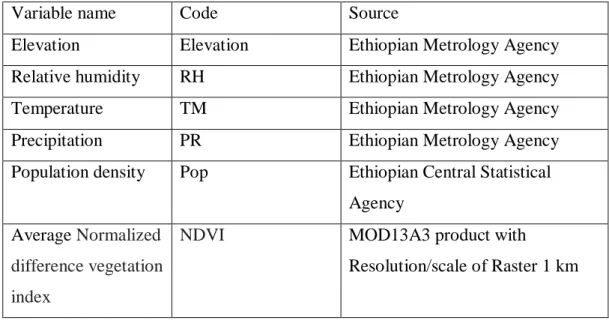
Table 2: Variables used in the research and their sources
Variable name Code Source
Elevation Elevation Ethiopian Metrology Agency Relative humidity RH Ethiopian Metrology Agency Temperature TM Ethiopian Metrology Agency Precipitation PR Ethiopian Metrology Agency Population density Pop Ethiopian Central Statistical
Agency Average Normalized
difference vegetation index
NDVI MOD13A3 product with
Resolution/scale of Raster 1 km
3.3 Data pre-processing and modeling
The Geographically Weighted Regression (GWR) modeling approach was applied for exploring the association among malaria cases and local spatial predictors across the study area. Figure 4 depicts the schematic overview of the methodology. The malaria cases data were tested for spatial autocorrelation, and the explanatory variables were obtained for the 679 wards by interpolation techniques as a first step. The subsections below detail each stage of the methodological framework.
9
coll
ec
ti
on
S
elec
ti
on
P
re
-p
roc
es
sing
of
da
ta
RESPONSE VARIABLE (Y: malaria cases )Altitude (X1) Precipitation (X2) Relative Humidity (X3) Temperature (X4) NDVI (X5) Interpolation EXPLANATORY VARIABLES Distribution of malaria incidence Spatial autocorrelation test
Da
ta
ana
lys
is
R
es
ult
Figure 3: Flow chart of the research approach
Source of data used for the study
EMA Ethiopian Public Health
Institute
Environmental data Malaria cases
(malaria indicators)
Data cleaning and normalization using R Local Moran’s I and Gi* statistics
Ordinary Least Squares (global model) &Test multicollinearity
Geographically Weighted Regression (local model)
S-GWR (mixed model)
Result and Interpretation
10 3.3.1 Environmental data
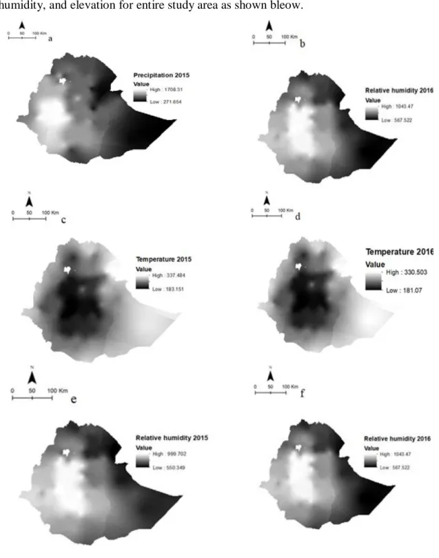
Figure 4 depicts the kriging interpolation result of precipitation, temperature, relative humidity, and elevation for entire study area as shown bleow.
11 Figure 4: Each explanatory variable mapped 2015(left) and 2016(right) in the study area.
All environmental risk factors variable were interpolated by using Kriging Spherical models as is illustrated in Table 3. Mean yearly interpolated climate factors data was used for analysis.
Table 3: Variogram models used for interpolation of explanatory variables with ordinary kriging
Dataset Model and parameters Model name and
values
Temperature model Spherical
nugget 0.001
range 4.2
Partial sill 1.067
Precipitation model Spherical
nugget 0.0009
range 5.24
Partial sill 0.998
Relative humidity model Spherical
nugget 0.0010
range 4.611
Partial sill 1.025
Elevation model Spherical
nugget 0.001049
range 4.0217
12 3.3.2 Data cleaning and normalization
Data cleaning and exploring were done by using R software. Logit and log malaria cases were used to discover if bivariate relationship were linear or not using B-splines explanatory analysis (Figure 17) in Appendix 7.1.
3.3.3 Spatial analysis of malaria
Initially, before applying regression analysis, we generate a malaria risk map, or hot-spots map, using local Gi* statistics (Yeshiwondim et al. 2009):
Where, wij is a geospatial weight matrix at a given distance lag in kilometers (d), (wij(d)) is 1 for location distance from j to i is within d; otherwise wij(d) is 0). The existence of hotspot of malaria indicators will be determined based on the value of Z-score. A high positive value of Z >1.96, showed that the position distinct i is surrounded by relatively high malaria cases region. In contrast, a high negative Z-score value indicates that the location separate i is surrounded by relatively low (cold spot) malaria incidence in distinct areas. Otherwise, random distribution of malaria cases for high and negative value of Z ≥-1.96 and ≤1.96 (Yeshiwondim et al. 2009). Anselin’s Local Indicators of Spatial Association (LISA) method, particularly the Local Moran’s I Statistic (Anselin 1995), was used to map the local clusters of high malaria cases. LISA calculates a measure of spatial association for each ward locations. A local Moran’s I autocorrelation statistic at the location i (Acharya et al. 2018)can be expressed as
where zi and zj are the standardized scores of attribute values for unit i and j, and j is among the identified neighbors of i according to the weights matrix wij.
3.3.4 Regression analysis
Geographically weighted regression (Ge et al. 2017) is a suitable method for spatially varying relationship data analysis. In regression data analysis, for example, ordinary
13 least squares (OLS), generally assume fixed relationships between dependent and independent variables in the study area. However, Geographically weighted regression (GWR) lets the regression parameters to differ locally by disseminating location-wise parameter estimates for all independent variables (Fotheringham et al. 2002). GWR determines the spatial variabiliy of coefficients within the study area, and the explanatory power of explanatory variables is spatially measured for local analysis (Ge et al. 2017). It has been widely used as a tool to explore non-stationarity, and its execution has been improved with new contributions, such as new sets of kernel functions (Chasco, García, and Vicéns 2007), best bandwidth selection (Páez, Uchida and Miyamoto, 2002; Ge et al., 2017), and optimum distance metric selection (Lu et al., 2015; Ge et al., 2017).
In past years, GWR has been used in several fields, for example, environmental science and meteorological science discipline (e.g., (Pasculli et al., 2014; Videras, 2014; Ge et al., 2017; Yao and Zhang, 2013), Geographic information science and Remote Sensing (e.g. (Gao and Li, 2011; Ge et al., 2017; Su, Xiao and Zhang, 2012; Wang, Kockelman and Wang, 2011), and mainly public health and disease (e.g. Ge et al., 2017; McKinley et al., 2013). In the studies with human health, the GWR methods have been applied to discover the spatial dissimilarities of heavy metals in the soil (McKinley et al. 2013), climate variables (Ge et al. 2017), air pollution (Jephcote and Chen 2012), and socioeconomic variables (Chi et al. 2013). The model GWR is appropriate for non-stationary variables (Fotheringham et al. 2002). In the first step, the average annual malaria cases in all two years (2015-2016) was tested for spatial heterogeneity (non-stationarity) with Global Moran’s I statistic.
In many studies, to deal with data with zero malaria cases, the malaria case data were adjusted by a Bayesian model (Ge et al. 2017). The malaria data we used had not consisted of a large number of locations with zero malaria cases; therefore, we didn’t apply the Bayesian model for this study.
In regression, multicollinearity could occur if one explanatory variable was a linear function of another explanatory variable and formerly observed in GWR modeling (Hasyim et al. 2018). The independent variables “altitude,” “relative humidity,” “precipitation,” “NDVI,” and “temperature” were tested for multicollinearity. To investigate the colinearity problem among the independent variables, we used indices that are based on the predicted variance of modeling Variance Inflation Factor (VIF)
14 (Halimi et al. 2014). We considered the most often applied criteria that establish that variables with VIF greater than 4 warrant further investigations, and those with VIF greater than 10 indicate serious multicollinearity.
Ordinary Least Squares was initially used before the GWR model to examine global statistical relationships between dependent and explanatory variables, including the multicollinearity assumption. At this level, the presence of local variation in relationships was not taken into account in regression.The OLS regression model was used to assess the global relationship between malaria cases and the selected envriomental risk factors. The method of least square expressed in the following equation (Acharya et al. 2018):
Where yi is the ith examination of the response variable, ajxij is the ith examination of the Kth explanatory variable, and εi is the error terms. The global model assumes that the rate of neighborhood ward i is independent of neighboring j and that residuals usually distributed in terms with zero mean.
Since the study area was characterized by spatial heterogeneity, we used the GWR model as an alternative to examine the local relationship between the dependent and independent variables (Hasyim et al. 2018). With the discussed dependent and independent variables, the GWR model can be formalized as
Where y is the value of malaria cases at the location u, xt is the value of explanatory variable t at the location u, βt (u) is the regression coefficient at the location u, and ԑ is the random error with mean 0 and variance σ².
In the GWR model, each explanatory variable has different regression parameters due to spatially varying parameters in weighted analysis regression (Mar’ah, Djuraidah, and Wigena 2017).
15 The GWR model that has both local and global parameters is known as Mixed Geographically Weighted Regression or Semi-parametric Geographically Weighted Regression (Nakaya et al. 2005). According to (Mar’ah et al. 2017), a stepwise procedure that allows all possible mixture of global and local parameters was tested, and the optimum mixed/semi-parametric model was selected based on the smallest corrected Akaike Information Criterion (AICc) value. The spatial variability test (F-Test) was used by the model to determine local parameters in the model (Mei, Wang, and Zhang 2006). The specified local and global parameters depend on the confidence interval of GWR coefficients (Mar’ah et al. 2017).
In the GWR models, a weight matrix is calculated to calibrate the model and distinguish the spatial association among nearby wards. A fixed Gaussian kernel function was applied for the weighting scheme (Hasyim et al. 2018). The optimal distance threshold was determined by minimizing the AICc of the model.
A Gaussian kernel is appropriate for fixed kernels as it can prevent the risk of there being no data within a kernel (Nakaya 2016). The golden search method was applied to decide the best bandwidth size for geographically weighting efficiently. The best bandwidth and the related weighting function were attained by selecting the smallest AICc score. The fixed Gaussian kernel for geographical weighting used in this study(Nakaya 2016) is as follows:
(4)
Where wij is the weight value of the observation at the location j to estimate the coefficient at location i, dij is the Euclidean distance between i and j, and b is the size
of the fixed bandwidth given by the distance metric. The positive [negative] association between response and explanatory variables can be indicated by a positive [negative] regression coefficient βt(u) of the explanatory variable t at the location u. If one explanatory variable Xt (i.e. environmental risk factor) has a positive [negative] coefficient at the location u, it means that when Xt increases at the location u, it is expected that the malaria cases(Y) increases [decreases] at the location u, assuming all other factors remain constant.
16 Finally, we applied Semiparametric Geographically Weighted Regression (s-GWR) models treating some predictors as global while others as local. The s-GWR model is expressed in the following equation (Fotheringham et al. 2002):
where for observation i, is the geographical location, are the ka
global coefficients associated with the set of global explanatory variables , are the kb local coefficient functions associated with the set of
local explanatory variables
The selected environmental variables (Elevation, precipitation, temperature, NDVI, and relative humidity) correspond to the explanatory variables, and the pre-processed annual average malaria cases is the response variable in the GWR and s-GWR models of 2015 and 2016. OLS regressions were also fitted for comparison purposes. Diagnostic information provided includes the overall R2, AICc, and the analysis of spatial autocorrelation of the residuals.
Some results of the GWR and s-GWR models (e.g., local R2, local coefficients, and estimated cases and residuals) were mapped using the ArcGIS10.6. Mapping local parameters make a straightforward interpretation based on recognized characteristics and spatial background of the research area (Goodchild and Janelle 2004). On the other hand, only mapping the predictor’s local coefficients does not provide a way of knowing whether they are significant anywhere on the study region (Matthews and Yang 2012). Accordingly, statistically significant wards where pseudo-t values exceed ± 1.96 were considered as relevant (Ehlkes et al., 2014; Acharya et al., 2018; Wabiri et al., 2016; Matthews and Yang, 2012).
17
4
RESULTS4.1 The spatial analysis and distribution of malaria Cases
A total of 19687.31 cases in 2015 and 456807.8 cases in 2016 in a total population of approximately 99,870,000 and 102,400,000 in Ethiopia were recorded in 2015 and 2016, respectively. This translates to overall annual malaria cases of 0.197 per 1000 and 4.461 per 1000 inhabitants in 2015 and 2016, respectively.
The malaria cases were distributed in the wards, as shown in Figure 5. The results of the global spatial autocorrelation test for the 2015 and 2016 years data showed significant spatial dependence in several wards for all yearly cases: minimum Moran’s I = 0.323, p < 0.05 (2015), and maximum Moran’s I = 0.514, p < 0.05 (2016). The significant local spatial autocorrelation result for malaria cases ensured the suitability of the malaria cases data as the response variable in GWR models. Local spatial autocorrelation of each year was assessed with local indicators of spatial association (LISA) (Anselin 1995), namely the Local Moran’s I statistic Figure 5 and the Getis-Ord Gi* statistic (Figure 6). The Local Moran’s I maps showed the spot regions (high-high) and cold-spot regions (low-low), where hot-spot location means the malaria cases of a particular spatial unit is high, and malaria cases of its surrounding units are also high, and cold-spot region implies the opposite.
18
c d
Figure 5 Local Moran’s I test maps of malaria cases and corresponding significance for 2015 (top) and 2016 (bottom).
The hot-spot locations of malaria cases in 2015 Figure 5a were the wards along the west, the northwestern part of the country, whereas the cold-spot were along the west, the central and southeastern part of the country. The hot-spot locations of malaria cases in 2016 Figure 5c were very high malaria cases in the wards along the northwest, and the west northern part of the country, whereas the cold-spot were wards along the western, central, and southeastern part of the country. A few zones exhibit local negative spatial autocorrelation where wards with low values of malaria cases correlate with high neighbouring values (10 and 9 Low-High wards in 2015 and 2016 respectively), and wards with high values of malaria cases correlate with low neighbouring values (8 High-Low wards in 2015).
Figure 6 depicts the annual malaria cases distribution in 2015 and 2016 at wards level in the country using Hot Spot Analysis (Getis-Ord Gi* statistic). Accordingly, in 2015 the yearly malaria cases hot-spot distribution was along the north and northwestern region of the country. In contrast, in 2016, the annual malaria cases hot-spot distribution was along the northern part of the county (Figure 6b). These results also highlight the spatial nonstationarity of malaria cases.
19 Figure 6. Hot-spot (Getis-Ord Gi* statistic) results of malaria cases in 2015 (a) and 2016 (b)
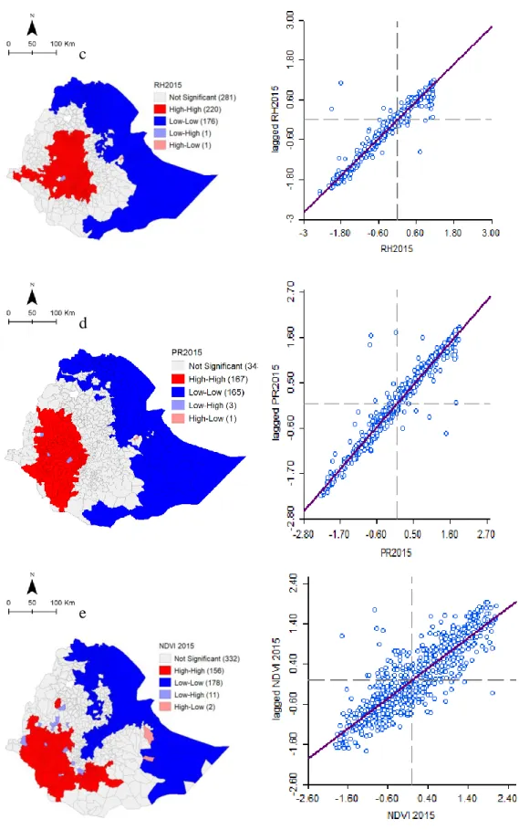
4.2 Spatial analysis of predictors
The explanatory variables were assessed using spatial autocorrelation, and it was found to be significant for five of the independent variables Figure 7. A local Moran’s I analysis result identified along with the hot-pot and cold-spot distributions of the five variables. The hot-spot locations of Elevation Figure 7a were the wards along the north-central part of the country. The temperature hot-spot areas were in
20 the southern-eastern, northeastern lowlands and western regions of the country as depicted in Figure 7b. Relative humidity hot-spot distribution was along the central areas of the country as drew in Figure 7c. Precipitation hot-spot distribution was wards along the Western and Central regions of the country Figure 7d. Figure 7e showed hot-spots in the normalized difference vegetation index (NDVI) distribution along the southwestern part of the country.
a
21 c
d
e
Figure 7: Distribution of selected explanatory variables with their corresponding local (1st column) and global Moran’s I tests (2nd column)
22 4.3 Ordinary Least Squares model
The coefficients of the Ordinary Least Squares models have the same value for all points within the study area (Table 4) and (Table 5). Thus, the global regression models could not capture the process for spatial heterogeneity and varying relationships in the data. In the 2015 model (Table 4), none of the regression coefficients is significantly different from zero at the 5% significance level (p-value>0.05), though the coefficient of temperature (TM2015) is significant at the 10% significance level. In the 2016 model (Table 5) all coefficients are significant at the 5% level (p-value0.05), except NDVI2016.
In the two models (2015, 2016), all independent variables have VIF<4, so there is no evidence of multicollinearity among them as shown in Table 4 and Table 5. Therefore, it is appropriate to use them in the local models.
Table 4: Summary of OLS Results - Model Variables for 2015
Variable Coefficient StdError
t-Statistic p-value Robust StdError Robust_t Robust p-value VIF Intercept -37.078 65.507 -0.566 0.571 71.985 -0.515 0.606 ……. Elevation -0.009 0.008 -1.120 0.262 0.009 -0.962 0.335 1.687 TM2015 3.083 1.598 1.930 0.053 1.777 1.735 0.083 3.416 RH2015 0.193 0.521 0.371 0.710 0.581 0.332 0.739 3.856 PR2015 0.246 0.166 1.481 0.138 0.198 1.242 0.214 3.252 NDVI2015 -0.002 0.002 -1.441 0.149 0.002 -1.589 0.112 2.208
Table 5: Summary of OLS Results - Model Variables for 2016
Variable Coefficient StdError t-Statistic p-value Robust StdError Robust_ t Robust p-value VIF Intercept -9252.87 2844.84 -3.252 0.001* 3677.108 -2.516 0.012* …… Elevation 2.895 0.34 8.451 0.000* 0.551 5.251 0.000* 1.731 TM2016 411.115 69.41 5.922 0.000* 100.407 4.094 0.001* 3.807 PR2016 6.261 4.97 1.258 0.208 2.211 2.831 0.004* 2.096 RH2016 -51.043 21.51 -2.372 0.018* 25.473 -2.003 0.045* 3.951 NDVI2016 -0.027 0.08 -0.331 0.741 0.053 -0.508 0.611 1.655
4.4 Geographically Weighted Regression model
The GWR models were used to explore the local effects of variables on malaria cases in all wards in 2015 and 2016. The independent variables were temperature,
23 elevation, relative humidity, precipitation, and predictor variable derived from remote sensing data (NDVI).
The pseudo-t statistics in the GWR model indicate the statistical significance of locally varying coefficients for the explanatory variables. Figure 8 depicts the spatial distribution of pseudo-t values for all independent variables for both years in the study area. Pseudo-t values were computed by dividing independent coefficient estimates by their standard errors, with statistical significance defined as a pseudo-t-value greater than or equal to 1.96 (positive relationship) or pseudo-t pseudo-t-value smaller than or equal to -1.96 (negative relationship) (Nakaya et al., 2005;Kuo et al., 2017). The non-significant coefficients are represented in yellow in Figure 8, with a statistically significant positive association in red/orange and negative statistically significant relationship in green/light green. Figure 9(a-e) and Figure 10(a-e) shows local coefficients for independent variables for both years in the GWR models. It effectively reveals how the direction and strength of the relationship between each predictor and response variable vary over space. Table 6 and Table 7 summarize the values of the maps of GWR local coefficients in Figure 9(a-e) and Figure 10(a-e), and also show global adjustment measures (R2, Adjusted R2 and AICc). Despite the higher Adjusted R2 in 2016 model, the 2015 model has a better global fit considering its lowest value of the AICc. All these results are further discussed below.
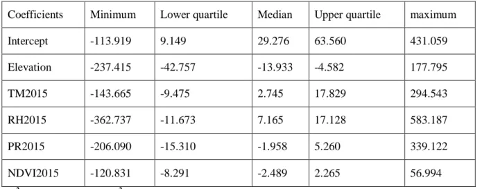
Table 6. Summary of the locally varying coefficients of the variables on the GWR model in 2015.
Coefficients Minimum Lower quartile Median Upper quartile maximum
Intercept -113.919 9.149 29.276 63.560 431.059 Elevation -237.415 -42.757 -13.933 -4.582 177.795 TM2015 -143.665 -9.475 2.745 17.829 294.543 RH2015 -362.737 -11.673 7.165 17.128 583.187 PR2015 -206.090 -15.310 -1.958 5.260 339.122 NDVI2015 -120.831 -8.291 -2.489 2.265 56.994 R2 = 0.630, Adjusted R2 =0.515, AICc= 7311.884
24 Table 7 Summary of the locally varying coefficients of the variables on the GWR model in 2016.
Coefficients Minimum Lower
quartile Median Upper quartile maximum Intercept -13284.062 5.503 15.931 30.822 9390.445 Elevation -4007.037 -15.514 -2.653 11.094 4683.572 TM2016 -4299.357 -11.299 0.523 16.990 4500.589 PR2016 -19773.517 -26.501 -5.672 1.107 5874.614 RH2016 -13530.506 -26.221 0.522 9.315 4867.645 NDVI2016 -798.797 -4.291 -0.748 6.899 10148.366 R2= 0.680, Adjusted R2= 0.608, AICc=12349.729
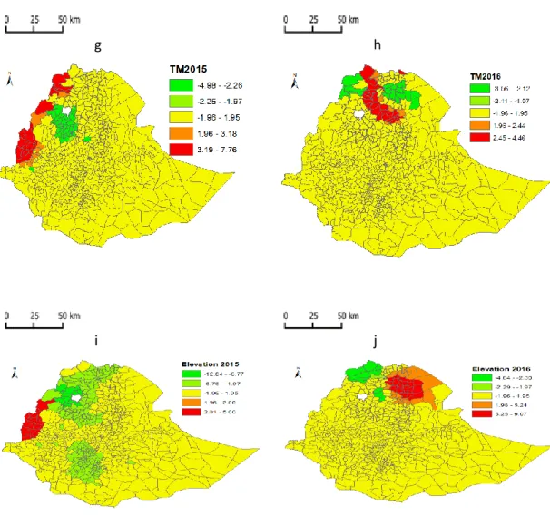
In 2015, temperature coefficients showed a positive and negative correlation with malaria case per wards and were significant in some wards located to the northwestern, southwestern part of the study areas Figure 8g. Elevation 2015 estimated coefficients showed a positive and negative relationship with malaria cases per ward and was significant in some wards located to the northern, southwestern, and southern part of the study areas (Figure 8i). In 2015, the estimated NDVI coefficients showed a positive and negative relationship with malaria cases per wards and were significant in some wards located to the northwestern, northeastern and southern part of the country Figure 8a. In 2015 precipitation estimated coefficients showed a positive and negative correlation with malaria cases per wards and were significant in some wards located to the western, northwestern, southwestern, and south-central parts of the study area (Figure 8c). In 2015 relative humidity estimated coefficients showed a positive and negative association with malaria cases per wards and were significant in some wards located to the northern and western part of wards in the study area (Figure 8d). In 2016 NDVI estimated coefficients depicted only positive correlation with malaria cases per wards and were significant in some wards located to the northeastern wards of the country (Figure 8b).
In 2016 Precipitation estimated coefficients showed an only negative relationship with malaria cases per wards and were significant in some wards located to the northern part of the country (Figure 8d). In 2016 relative humidity, temperature, and elevation estimated coefficients depicted a positive and negative correlation with malaria cases per wards and were significant in some wards located to the northern part of the country (Figure 8h, f, and j).
25
a b
c d
26
g h
i j
Figure 8. Pseudo t-values for independent variables in 2015 (left) and 2016 (right)
a b
27 e
Figure 9. GWR local coefficients of the 2015 model (a-e)
28
c d
e
Figure 10.GWR local coefficients of the 2016 model (a-e)
In 2015 temperature is significantly and positively related to malaria cases in the following 28 Wards:
Gidami, Jimma Horo, Dale Wabera,
Gawo Kebe, Babo, Gudetu Kondole,
Maok Omo, Begi, Kiltu kara,
Mana Sibu, Bambasi, Assosa, Menge, Homosha, Biligidillu, Sirba Abaya, Kumuruk, Sherkole,
Guba, Anfilo, Yama Logi welel,
Hawa Gelan, Dale sadi, Ayira Guliso, Boji Chekorsa, Nejo, Agalmoeti,
29 Qura, Mirab Armacho, Tsegede,
Kafta Humera, Tach Armacho.
Temperature was also significant and negatively related to malaria cases in the following 31 wards (Figure 8g):
Amuru, Debra Elias, Guzamn,
Michakel, Bure, Wemberama,
Dembecha, Senan, Jabi Tehnan,
Ankasha, Guagusa, Dega Damot,
Bibugn,Banja, Sekela, Quarit, Gonje, Fagta lakoma, Yilmana Densa, Dangila,
Pawe, Anchefer, Mecha,
Bahirdar Zuria, Dera , Jawi, Fogera, Libo Kemekm, Takusa ,
Dera, Bure, and Alfa.
Elevation 2015 estimated coefficient was significant and positively related to malaria cases in the following 18 wards in the country:
Gidami, Jimma Horo, Dale Wabera, Gawo Kebe, Babo, Gudetu Kondole,
Maok Omo, Begi, Kiltu kara,
Mana Sibu, Bambasi, Assosa, Menge, Homosha, Biligidillu, Sirba Abaya,
Kumuruk, Sherkole and Guba.
Moreover, Elevation 2015 was also significant and negatively related to malaria cases in the following 160 wards in the country (Figure 8i):
Asgede Tsimbila, Medebay, Naeder Adet, Kola Temben, Degua Temben, Hawzen, Tahtay koraro, laelay Maychew, Adwa,
Afeshum, Erop, Gulomekeda,
Ahferom, Mereb Leka, laelay Adiyabo, Mirab Armacho, Tsegede, Debark,
Addi Arekay, Beyeda, Tselemt,
Welkait, Alfa, Fogera,
Farta, Lay Gayint, Libo Kemkem,
Ebenat, west Belesa, East Belesa,
Takusa, Chilgam, Dembia,
GonderZuria, Lay Armachewo, Wegera,
Dabat, Metema, Danguara,
Pawe, Dangila, Mecha,
yilmana Densa, West Esite, Dera, Bahirdar Zuria, Debub Anchefer, Jawi,
Limu, Ababo, Baso liben,
Awabel, Dejen, Wara Jarso,
Dera, Wegde, Debresina,
Shebel Bereta, Dejen, Awabel,
30 Guzamn, Debre Elias, Bure,
Dembecha, Michakel, Senan,
Debay, Telatgen, Enemay,
Enar Enawa, Jabi Tehnan, Bure Dembecha,
Wemberma, Guangua, Ankasha,
Dega Damot, Sekela, Quarit,
Sekela, Mandura, Fagta Lakoma,
Ameya, Nono, Goro,
Tocha, Mareka, Gena Bosa,
Boloso Bombe, Kacha Bira, Tibaro,
Omo Nada, Sekoru, Yem, Gibe,
Endiguagn, Admi Tulu, Selti,
Ezha, Cheha, Chora,
limu kosa, Sekoru, Tiro Afeta,
Ameya, Nono,chora, Amaro SP,
Koochere, Gedeb, Kercha,
Bule Hora, Hambela, Wamena,
Borke, Arba Minch Zuria, kemba,
zala, Daramalo, Dita,
Chencha, Abaya, Dila Zuria,
Wenagol, Bule, Yirgachefe,
Afele Kola, Bore, Dara,
Hulla, Bursa, Dale,
Humbo, Loka Abaya, Zala,
Denibu Gofa, Kucha, Boreda,
Sodo Zuria, Damot, Boricha,
Boloso Sore, Bomb, Siraro,
Awasa Zuria, Goro, Arsi Negeli,
limu, Kacha biraa, loma Bosa,
Ofa, Kindo Dida, Mareka,
Tibaro, Dune, Daniboya,
Dedo, Omo Nada, Goro,
Shashemene zuria And Bure
In 2015 the estimated NDVI local coefficient was significant and positively related to malaria cases in the following 15 wards in the country:
Gaz gibla, Alamata, Olfa,
Sekota, Endamehoni, Raya Azebo,
Yalo, Teru, Alaje,
Megale, Erebti, Hintalo Wejirat,
Saharti Samre, Ab Ala, and Enderta. NDVI also significant and negatively related to malaria cases in the following 54 wards in the country (Figure 8a):
31
Mereb leke, Quara, Takusa,
Chilga, Dembia, Loma bosa,
Kindo dida, Ofa, Sodo zuria,
Kindo koysha, Damot sore, Damot gale, Damot pulasa, Mareka, Tocha, Gena Bosa, Boloso Bombe, Boloso sore, Badawacho, Tibaro, Kacha Bira, Hadero Tubito, Dune,Soro, Doya,
Gena, Daniboya, Shashogo,
Dedo, Omo Nada, Yem,
Gembora, LImu, Analemmo,
Sekoru, Gibe, Tiro Afeta,
sekoru, Alfa, Geta,
wilbareg, Yama logi welel, Jimma Horo, Gawo kebe, Dale wabera, Gudetu condole,
Babo, Gumurk, Homosha,
Pawe, and Metema
Achefer,
Enemorina Eaner
Jawi,
In 2015 precipitation estimated local coefficient was significant and positively to malaria cases in the following 16 wards in the country:
Kurmuk, Homosha, Assosa,
Bambasi, Begi, Maok omo,
Guba,shebel berta, Wegede, Enarj enawaga,
Debresina, Enbise sar midir, Mehal sayint,
Sayit, Simada, Tach gayint
and Dawunt
Precipitation was also significant and negatively related to malaria cases in the following 49 wards in the country (Figure 8c):
Cheta, Decha, Ela,
Melekoza, Geze gofa, Ayida,
Zala, Darmalo, Denibu gofa,
Esira,Yaso, Ibantu, Dibat,
Bulen, Guangua, Ankasha,
Bure, Wemberma, Madura,
Banja, Fagta lakoma, Mecha,
Dangila, Pawe, Anchefer,
Bahirdar Zuria, Yilana densa, Dera, Alfa,
Jawi, Takusa, libo kemekem,
Ebenat, Metema, Chilga,
Dembia, Gonder zuria, Belesa,
Wegera, Lay armacho, Janamora,
Dabat, Armarcho, Tsegede,
Debark, Addi Arekay, Welkait, Addi arekay, Kefta humera, Dera and Bure.
32 In 2015 relative humidity was significant and positively related to malaria in the following 43 wards in the country.
Metema, Chilga, Lay Armacho,
Mirab Armacho, Tach Armacho, Tsegede,
Dembia, Gonder Zuria, West Belesa,
Wegera, Dabat, Janamora,
Debark, Addi Arekay, Tselemt,
Beyeda, Welkait, Kafta Humera,
Asgede Tsimbila, Kola Temben, Medebay,
Tshtay koraro, Maychew, Adwa,
Laelay Adiyabo, Mereb Leke, Tahtay Adiyabo,
Gidami, Jimma Horo, Dale Wabera,
Yama logi Wele, Gawo Kebe, Begi,
Gudetu Kondole, Babo, Nejo,
Mana Sibu, Kiltu Kara, Agalometi,
Daramalo, Dita, Chenech
and Mirab Abaya.
Relative humidity was also significant and negatively related to malaria Cases in the following 32 wards (Figure 8e):
Quara, Guba, Dangura,
Pawe, Dangila, Fafata lakoma,
Sekela, Quarit, Gonje,
Yilmana dense, Mecha, Anchefer, Bahirdar Zuria, Dera, Fogera,
Amuru, Debre Elias, Guzamn,
Michakel, Senan, Debay Telatgen,
Michakel, Dembecha, Bure,
Wembera, Daga damot, Bibugn, Hulet Ej Enese, Quarit, Ankasha,
Guangua, Guagusa And shiludad.
In year 2016 NDVI was significant and positive related to malaria cases in the following 50 wards in the country:
Sahla, Ziquala, Saharti Samre,
Alaje, Hintalo Wejirat, Megale,
Erebti, Afdera, Beyeda,
Tanqua Abergele, Abala, Enderta,
Degua Temben, Kola Temben, Kelete Awelallo, Atsbi Wenberta, Koneba, Berahle,
Werei leke, Hawazen, Sekota, Ganta Afeshum, Dalul, Berahle, Lay Gayint,
Dawunt, Wadla, Delanta,
Ambasel, Habru, Worebabu,
Chifra, Ewa, Guba Lafto,
Meket, Bugna, Lasta,
33
Awra, Aalmata, Gaz gibla,
Dehana, Ofla, Yalo,
Teru, Raya Azebo, Endamehoni,
SaesieTs aedaemba
and Erob.
NDVI also significant and negatively related to malaria cases in the Tahtay Adiyabo, Laelay Adiyabo and Mereb Leke wards (Figure 8b).
Precipitation estimated local coefficient showed only negative relationship with malaria cases per wards and was significant in thefollowing 58 wards (Figure 8d):
Ambasel, Tach Gayint, Farta, Lay Gayint,
Meket, Wadla, Delanta,
Worebabu, Chifa, Habru,
Guba lafto, Ewa, Awra,
Meket, Ebenat, Gugna,
Lasta, Gidan, Kobo,
Gulina, Alamata, Ofla,
Gaz Gibla, Dehana, Belesa,
Wegera, Ziquala, Sekota,
Enamehoni, Yalo, Teru,
Sahla, Janamora, Debat,
Tsegede, Debark, Addi arekay,
Welkait, keftay Humera, Tahtay Adiyabo, laelay Adiyabo, Mereb leke, Maychew, Adwa, Kola Temben, Wereri leke , Hawzen, Ganta Afeshum, Tselmti, Beyeda, Tanqua Abergele, Enderta ,
Abala , Erebti, Afdera,
Berahle, Koneba, kelete Awalalo
and Berahle.
Relative humidity was significant and positively related to malaria cases in the Tahtay Adiyabo and, Laelay Adiyabo Wards Moreover; it was significant and negatively related to malaria cases in the following 52 wards (Figure 8f).
Metema, Tach Armacho, Lay armacho, Tsegede, Mirab Armacho, Kaftay Humura, Tanqua Abergele, Enderta, Wegera,
Dabat, Debark, Janamora,
Beyeda, Sahla, Ziquala,
Endamehoni, Hintalo Wejirat, Abala,
Erebit, Worebabu, Chira,
Habru, Ewa, Awra,
Guba lafto, Gidan, kobo,
Gulina, Teru, Yalo,
Alamata, Gaz gibila, Dehana,
Sekota, Ofla, Tselemt,
34
Koneba, Berahle, Daul,
Hawazen, Werei leke, Naeder Adet,
Ganta afsshum, Erob, Dalul,
Gulomekede, Ahferom
. Saesis Ts
sedaemba,
and Welkait Temperature was significant and positively related to malaria cases in the in the following 26 wards in the country.
Dawunt, Ambasel, Delanta,
Wadla, Guba Lafto, Maket,
Laygayint, Bugna, Ebenat,
Gidan,Kobo, Lasta, Gaz,
Gibla, Dehana, Belesa,
Wegera, Dabat, Janamora,
Sahla, Debark, Addi Arekay,
Tselemti, Asgede tsimbila, Tahtay Adityabo, Tahtay Koraro and Erop.
Temperature also significant and negatively associated with malaria cases in the following 17 wards (Figure 8h).
Mirab Armacho, Tsegede, Kafta Humera,
Endameoni, Alaje, Teru,
Megale, Erebti, Abala,
Hintalo Wejirat, Saharti Samre, Abergele,
Tanqua Abergele, Degua Temben, Kola Tamben,
kelele Awelalo ,andAtsbi Wenberta.
Elevation was significant and positively related to malaria cases in the Delanta, Ambesal, Habru, Guba lafto, Chifa, Dubti, Ewa, Awara, Gulina, Kobo, Lasta, Gas Gibla, Almata, Ofla, Yalo, Teru, Afdera, Raya azebo, Sekota, Ziquala, Abergele, Alaje, Hintalo Wejrat, Megale, Erebti, Saharti Samre, Tanqua Abergele, Enderta, Degua Temben, Kola Temben, Werei leke, Hawzen, Atsbi Wenberta, Saesie Ts aedaemba, koneba, Berahle, and Dalul Wards. Moreover, Elevation is significant and negatively related with malaria cases in the Kafta Humera, Tsegede, Welkait, Asgede Tsimbila, Tselemti, Tahtay koraro, Tahtay Adiyabo, laelay Adiyabo, East Belesa, Ebenat, and Lay Gayint Wards as it depicted in Figure 8j.
The observed malaria cases map in 2015 (Figure 11a) should be compared with caution with the estimated map (Figure 11b), as well as the observed cases in 2016 (Figure 11c) with the estimated cases in 2016 (Figure 11d). According to the above discussion, the models’ coefficients are not relevant in a large number of wards, thus the predictive power of the models is low in most of the country. However, it is
35 important to point out that the models were not developed for prediction purposes. The usefulness and aim of the models is to identify relevant varying relationships between malaria cases and environmental variables.
a b
c d
Figure 11. Observed (a) and GWR estimated (b) malaria incidence in 2015; observed (c) and GWR estimated (d) malaria incidence in 2016
Table 8 depicts the comparison of the GWR and OLS models based on several indicators. For both years, the sum of the residuals of squares (RSS) was summarized to evaluate the model error, and Global Moran’s I of residuals were tested along with the associated significance levels. The AICc values showed that the GWR model of each year fitted better than the corresponding OLS models. The spatial autocorrelation of residuals was not entirely removed in the 2016 GWR model, but the Global Moran’s I statistic was closer to zero in GWR than in the OLS models.
36 Table 8 Comparison of goodness-of-fit results and residual analysis of the GWR and OLS models
Year AICc Adjusted R2 RSS Global Moran’s I of
residual (significance-score)
GWR OLS GWR OLS GWR OLS GWR OLS
2015 7311.88 7683.95 0.515 0.012 715.43 3199364.47 0.007 (p=0.143, Z=1.463) 0.395 (p=0.000, Z=10.662) 2016 12349.73 12772.77 0.608 0.182 2250710287 5753288780 -0.104 (p=0.020, Z=-2.319) 0.316 (p=0.000, Z=23.683)
Global Moran’s I results showed (Table 8) there is significant autocorrelation in the residuals of the GWR model in 2016, and authenticates the variables we considered in this study were unable to appropriately predict the malaria cases distribution spatially in the entire study area. That was due to the scarce population in some wards or missing explanatory variables. In contrast, the Global Moran’s I results of spatial autocorrelation of residuals of the 2015 model was not statistically significant so that the model was well specified.
4.5 Semiparametric Geographically Weighted Regression
Semiparametric Geographically Weighted Regression (s-GWR) models were investigated. The GWR model with all local variables (before L -> G selection) was compared with s-GWR models (after L -> G selection), where local variables were step by step selected to become global variables. The best s-GWR models had an AICc of 7273.689 in 2015, and 12304.718 in 2016 (Table 9), thus they performed better than the GWR models (Table 8). The s-GWR models were further used to explore the local and global relationships of the explanatory variables in connection to malaria case.
37 Table 9 Comparison of GWR and s-GWR models performances based on AICc
Year Model AICc Improvement
2015 GWR model (before L -> G selection) 7311.884 38.194 S-GWR model (after L -> G selection) 7273.689
2016 GWR model (before L -> G selection) 12349.729 45.010 S-GWR model (after L -> G selection) 12304.718
Table 10 reviews the result of GWR 4.0 (Nakaya et al., 2005;Nakaya, 2016), where contrast of OLS, GWR, and s-GWR in terms of AICc, R2, and adjusted R2. The OLS model explained only 1.2% in 2015 and 18.2% in 2016 of the variability of malaria cases, whereas the variability explained by the GWR models increased to 51.5% in 2015 and 60.9% in 2016, and a little more with the s-GWR models (53.8% in 2015, and 62.4% in 2016). The model fit was significantly improved with the s-GWR model, reducing the AICc values from 7684 to 7274 in 2015, and from 12773 to12305 in 2016. In summary, both s-GWR models performed better than the other competing models, thus they are considered the final models for malaria cases in this study.
Table 10 Comparison of OLS, GWR and s-GWR models performances based on goodness-of-fit measures
Year Fitness measures OLS
(global model) GWR (local model) s-GWR (mixed model) 2015 AICc 7683.95 7311.88 7273.69 R2 0.021 0.630 0.642 Adjusted R2 0.012 0.515 0.538 2016 AICc 12772.77 12349.73 12304.72 R2 0.189 0.683 0.685 Adjusted R2 0.182 0.609 0.624
The outcome of geographic variability test and local to global variable selection approach were based on DIFF of Criterion (Table 11 and Table 12) suggesting no spatial variability in the negative coefficient of NDVI in 2015, and negative coefficient of elevation and positive coefficient of temperature in 2016 (Nakaya 2016). Therefore, NDVI is a global explanatory variable, while the other four variables have a local varying explanation power in the 2015 model. In 2016, both elevation and temperature variables remained as global, while the other three independent variables are local.
38 The s-GWR model with NDVI as global predictor and elevation, temperature, precipitation, and relative humidity as local predictors corresponds to the final model found in 2015. In 2016, s-GWR model with elevation and temperature as global predictors and NDVI, precipitation and relative humidity as local predictors is the final model.
Table 11 Summary of s-GWR model coefficients in 2015 Global coefficients
Variable Estimate Standard Error t(Estimate/SE) DIFF of Criterion
NDVI2015 -3.560280 3.673756 -0.969112 33.827555 Local Coefficients
Variable Minimum Lower quartile Median Upper quartile maximum
Intercept -191.420 7.910 27.407 69.213 516.043 -132.546712 Elevation -254.355 -41.107 -14.286 -4.255 209.723 -26.453838 TM2015 -171.932 -12.620 1.321 16.662 505.169 -16.845405 RH2015 -436.018 -13.593 6.545 18.316 745.869 -14.245095 PR2015 -286.025 -15.893 -1.410 8.455 464.719 -5.695182 R2 = 0.642, Adjusted R2 =0.578, AICc= 7273.690
Table 12 Summary of s-GWR model coefficients in 2016 Global coefficients
Variable Estimate Standard Error t(Estimate/SE) DIFF of Criterion
Intercept -4.715983 259.525511 -0.018172 3.588635
Elevation -69.872590 153.268985 -0.455882 17.736322
TM2016 263.031167 237.138194 1.109189 8.655711 Local Coefficients
Variable Minimum Lower quartile Median Upper quartile maximum
PR2016 -29917.885 -76.106 3.564 57.030 1709.727 -49.857796
RH2016 -11305.206 86.091 226.052 292.885 7926.942 -16.984620
NDVI2016 -1485.792 -119.889 -32.930 21.994 13194.320 -55.513555
R2 = 0.685, Adjusted R2 =0.624, AICc= 12304.719
The local estimated coefficients variation and associated t statistics are shown in (Figure 12, Figure 13, Figure 14, and Figure 15) below.
39
a b
c d
Figure 12.S-GWR Pseudo t-values for independent variables in 2015 with significance levels