A Consumer Staples behemoth
- The acquisition of
Kimberly-Clark by Kraft-Heinz
Daniel Ricardo
Student number: 152416003
Dissertation written under the supervision of António Luís Borges de
Assunção
Dissertation submitted in partial fulfilment of requirements for the MSc in
Finance program, at the Universidade Católica Portuguesa, September 2018.
i
Abstract
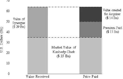
The main purpose of this dissertation is to study the hypothesis of an acquisition in the consumer staples sector, between Kraft-Heinz (the acquirer) and Kimberly-Clark (the target). Kraft-Heinz is a consumer staples company that recently completed the integration of a past merger, and is rumored to be looking for new targets to acquire. Its owners traditionally seek to acquire companies within the same industry, with strong brands and improvable operating margins. Kimberly-Clark is a company belonging to the consumer staples industry and the owner of several well-known brands. While it is smaller than Kraft-Heinz, it is expected to generate higher revenue growth in the foreseeable future, and its operational profitability possesses room for improvement. The combination of the two companies would allow for small increments in revenues, through combined scale and market power, and lead to operational improvements in Kimberly-Clark, following the Kraft-Heinz’ battle-hardened methods and culture. The combined company would also invest heavily in state-of-the-art facilities, while divesting older plants and reducing work-force. The expected synergies arriving from the deal were valued at $28 906 Million. The transaction assumes an all-cash friendly offer of $49 888 Million for 100% of Clark, representing a premium of 40.8% over Kimberly-Clark’s stock price.
Abstrato
O principal objetivo desta dissertação é estudar a hipótese de uma aquisição no setor dos bens de primeira necessidade, entre a Kraft-Heinz (o comprador) e a Kimberly-Clark (o alvo). A Kraft-Heinz é uma empresa do setor de bens de primeira necessidade que recentemente finalizou a integração de uma fusão anterior, e correm rumores de que se encontra à procura de novas empresas para adquirir. Os seus donos procuram tradicionalmente adquirir empresas dentro da mesma indústria, com marcas reconhecidas e margens operacionais que possam ser melhoradas. A Kimberly-Clark é uma empresa pertencente ao setor dos bens de primeira necessidade e dona de várias marcas famosas. Embora seja mais pequena que a Kraft-Heinz, é espectável que obtenha uma maior taxa de crescimento das suas receitas, e a sua rendibilidade operacional possui margem para melhorias. A combinação das duas empresas irá permitir pequenos incrementos nas receitas, através de economias de escala e aumento do poder negocial, e também a melhoria operacional da Kimberly-Clark, através da aplicação da metodologia e cultura organizacional da Kraft-Heinz. A empresa combinada irá também investir fortemente em fábricas topo de gama, ao mesmo tempo que irá descontinuar fábricas antigas e reduzir a sua força de trabalho. As sinergias resultantes da transação são avaliadas em $28 906 Milhões. A transação assume uma oferta amigável, totalmente em numerário, de $49 888 Milhões, por 100% da Kimberly-Clark, o que representa um prémio de 40.8% acima do preço atual das suas ações.
Keywords: Acquisition, Synergies, Premium, Consumer Staples Author: Daniel Jorge Carvalho Ricardo
Title: A Consumer Staples behemoth – The acquisition of Kimberly-Clark by Kraft-Heinz
ii
Acknowledgments
First of all, I would like to thank Católica-Lisbon School of Business and Economics, for the exceptional last two years, for giving me the possibility of partaking in such a challenging and rewarding program as the MSc in Finance, and for allowing me to pursuit a dissertation in my field of choice, Mergers and Acquisitions.
Secondly, I would like to thank my supervisor, António Luís Borges de Assunção, for his counseling, availability, and insightful remarks, which undoubtedly enrichened this dissertation.
I would also like to thank my friends whom, across the years, have encouraged me, and have been there for me.
Last but not least, I would like to thank my parents, for their encouragement, for all the lessons they have taught me, and for their unconditional support.
iii
TABLE OF CONTENTS
LIST OF FIGURES --- VII LIST OF ABBREVIATIONS ---VIII
1. Introduction ... 1
2. Literature Review ... 2
2.1. M&A --- 2
2.1.1. Why it happens --- 2
2.1.2. How it benefits society --- 2
2.1.3. Synergies --- 3
2.1.4. M&A in Consumer Staples --- 4
2.2. Valuation Methods --- 4
2.2.1. Discounted Cash Flow methods --- 4
2.2.1.1. Weighted Average Cost of Capital --- 5
2.2.1.2. Adjusted Present Value --- 5
2.2.2. The Method of Comparables --- 6
2.2.3. Remarks on the usage of each method --- 6
2.3. Form of Payment --- 7
2.4. Approaching the target --- 8
2.5. Post-Merger Integration --- 8
3. Industry Analysis ... 9
3.1. The Industry and its segments --- 9
3.2. Competitive Analysis --- 10
3.3. Future trends --- 10
4. Company Analysis ... 11
4.1. The Kraft-Heinz Company--- 11
4.2. Kimberly-Clark Corporation --- 13
5. Valuation of each individual company ... 16
5.1. Kraft-Heinz--- 16
5.1.1. Kraft-Heinz Forecast assumptions --- 16
5.1.2. Kraft-Heinz Valuation and Cost of Capital --- 19
5.1.2.1. Kraft-Heinz DCF/WACC Valuation --- 19
5.1.2.2. Kraft-Heinz DCF/APV Valuation --- 21
iv
5.1.3. Kraft-Heinz Sensitivity and Scenario Analysis --- 23
5.2. Kimberly-Clark --- 25
5.2.1. Kimberly-Clark Forecast assumptions --- 25
5.2.2. Kimberly-Clark Valuation and Cost of Capital --- 27
5.2.2.1. Kimberly-Clark DCF/WACC Valuation --- 27
5.2.2.2. Kimberly-Clark DCF/APV Valuation --- 29
5.2.2.3. Kimberly-Clark Comparables Valuation --- 30
5.2.3. Kimberly-Clark Sensitivity and Scenario Analysis --- 30
5.3. Valuation Results--- 31
6. Deal Rationale ... 32
7. Synergies ... 33
7.1. Combined company without synergies --- 33
7.2. Estimation of Synergies --- 33
7.2.1. Revenue synergies --- 34
7.2.2. Cost synergies --- 34
7.3. Combined company with synergies --- 36
7.4. Synergies Valuation; Cost of capital of the Combined firm --- 37
7.4.1. DCF/WACC --- 37
7.4.2. DCF/APV --- 37
7.5. Sensitivity and Scenario Analysis --- 39
8. Negotiation ... 40
8.1. Premium to pay --- 40
8.2. Financing the Deal --- 41
8.3. Purchase Price Allocation --- 41
8.4. Form of payment --- 41
8.5. Approaching the Target --- 42
9. Post-Merger Integration ... 43
10. Conclusion ... 44
11. Appendices ... 45
11.1. Kraft-Heinz’s Historical Statement of NOPLAT --- 45
11.2. Kraft-Heinz’s Historical Statement of Invested Capital --- 45
11.3. Kraft-Heinz’s Historical Statement of Free Cash Flow --- 46
11.4. Kraft-Heinz’s Historical Analysis --- 47
v
11.6. Kimberly-Clark’s Historical Statement of Invested Capital --- 48
11.7. Kimberly-Clark’s Historical Statement of Free Cash Flow --- 49
11.8. Kimberly-Clark’s Historical Analysis--- 49
11.9. Kraft-Heinz’s Performance Drivers --- 50
11.10. Kraft-Heinz’s Forecasted Statement of NOPLAT --- 51
11.11. Kraft-Heinz’s Forecasted Statement of Invested Capital --- 52
11.12. Kraft-Heinz’s Forecasted Statement of Free Cash Flow --- 53
11.13. Kraft-Heinz’s Forecasted Performance Analysis --- 53
11.14. Kraft-Heinz’s Cost of Capital --- 54
11.15. Kraft-Heinz’s DCF/WACC Valuation --- 55
11.16. Kraft-Heinz’s APV Valuation --- 56
11.17. Kraft-Heinz’s Comparables Valuation --- 57
11.18. Kraft-Heinz’s Sensitivity Analysis --- 57
11.19. Kraft-Heinz’s Scenario Analysis --- 58
11.20. Kimberly-Clark’s Performance Drivers--- 59
11.21. Kimberly-Clark’s Forecasted Statement of NOPLAT --- 60
11.22. Kimberly-Clark’s Forecasted Statement of Invested Capital --- 61
11.23. Kimberly-Clark’s Forecasted Statement of Free Cash Flow --- 62
11.24. Kimberly-Clark’s Forecasted Performance Analysis --- 62
11.25. Kimberly-Clark’s Cost of Capital--- 63
11.26. Kimberly-Clark’s DCF/WACC Valuation --- 64
11.27. Kimberly-Clark’s APV Valuation --- 65
11.28. Kimberly-Clark’s Comparables Valuation --- 66
11.29. Kimberly-Clark’s Sensitivity Analysis--- 66
11.30. Kimberly-Clark’s Scenario Analysis --- 67
11.31. Revenue Synergies --- 68
11.32. Cost Synergies --- 68
11.33. Combined firm’s Cost of Capital --- 68
11.34. Combined Company’s Forecasted Statement of NOPLAT --- 69
11.35. Combined Company’s Forecasted Statement of Invested Capital --- 70
11.36. Combined Company’s Forecasted Statement of Free Cash Flow --- 71
11.37. Combined Company’s Forecasted Performance Analysis --- 71
11.38. Combined Company’s Interest Coverage ratio, Credit Rating, Spread, and Probability of Default --- 71
vi
11.39. Combined Company’s APV Valuation --- 72
11.40. Synergies Sensitivity Analysis --- 73
11.41. Relationship between Interest Coverage ratio, Credit Rating, Spread, and Probability of Default --- 73
11.42. Purchase Price Allocation --- 73
11.43. Synergies Scenario Analysis --- 74
vii
LIST OF FIGURES
Figure 1 – Market Capitalization of the Sub-sectors in the Consumer Staples Sector (Fidelity
Investments, 2018) --- 9
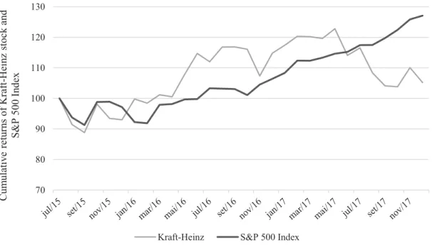
Figure 2 – Cumulative returns of Kraft-Heinz’s stock, compared to the S&P 500 Index (The Wharton School, University of Pennsylvania, 2018) --- 11
Figure 3 – Largest companies in the Consumer Staples Sector (Thomson Reuters Eikon, 2018) --- 12
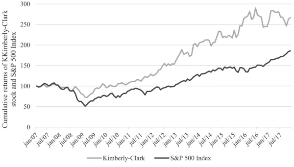
Figure 4 – Cumulative returns of Kimberly-Clark’s stock, compared to the S&P 500 Index (The Wharton School, University of Pennsylvania, 2018) --- 14
Figure 5 – Kraft-Heinz’s and Kimberly Clark’s Valuation results --- 31
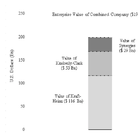
Figure 6 – Breakdown of Combined Company’s Value --- 38
viii
LIST OF ABBREVIATIONS
M&A Mergers and Acquisitions
GISC Global Industry Classification Standard
LBO Leveraged Buyout
DCF Discounted Cash Flow
EV Enterprise Value
FCF Free Cash Flow
FCFF Free Cash Flow to the Firm
WACC Weighted Average Cost of Capital
APV Adjusted Present Value
CAPM Capital Asset Pricing Model
YTM Yield to Maturity
PV Present Value
NPV Net Present Value
ITS Interest Tax Shield
EBITDA Earnings Before Interest, Taxes, Depreciation, and Amortization
EBIT Earnings Before Interest and Taxes
PMI Post-Merger Integration
NOPLAT Net Operating Profit Less Adjusted Taxes
ROIC Return on Invested Capital
RONIC Return on New Invested Capital
ROA Return on Assets
ix
COGS Cost Of Goods Sold
Gross Margin COGS / Total Revenues EBITDA margin EBITDA / Total Revenues
EBIT Margin EBIT / Total Revenues
NOPLAT margin NOPLAT / Total Revenues
SG&A Selling, General, and Administrative Expenses
PPE Property, Plant, and Equipment
NPPE Net Property, Plant, and Equipment
GPPE Gross Property, Plant, and Equipment
Payout Ratio Dividends/Net Income
Capex Capital Expenditures
Interest Coverage Ratio
EBITDA / Interest Expenses
PPA Purchase Price Allocation
NCI Non-Controlling Interests
1
1. Introduction
In early 2017, The Kraft-Heinz Company announced its intention to acquire Unilever. The transaction failed, but signaled Kraft-Heinz’ intentions of acquiring another company in the Consumer Staples sector.
In this dissertation, the hypothesis of Kraft-Heinz acquiring Kimberly-Clark Corporation, the owner of brands such as Huggies ® and Scottex ®, is studied. Both companies are studied and evaluated as stand-alone businesses, and as a combined firm, created by the acquisition of the latter by the former. To analyze the combined company, a special emphasis is given to the synergies that could emerge from the transaction.
In Chapter 2, a review of the existing literature on the topic of Mergers and Acquisitions, is performed, covering topics ranging from the reasons behind M&A, to valuation techniques, and post-merger integration.
In Chapter 3, the industry in which both companies operate is analyzed, with a focus on its business segments, competition, and future outlooks.
Next, in Chapter 4, each company is introduced, with a brief historical analysis.
Chapter 5 is dedicated to the valuation of each firm as a stand-alone business. To this end, each firm’s financial statements are projected for next fifteen years, and a detailed explanation on the process and assumptions made is presented. Each company is subsequently valuated using three different and complementary techniques.
In Chapter 6, the rationale behind the transaction is presented. Chapter 7, in turn, is solely dedicated to the synergies created by the deal and to the valuation of the combined company. Chapter 8 discusses the negotiation process, and attention is given to the price to pay for the acquisition, the sources of financing, the method of payment, and how to approach the target. Chapter 9 is dedicated to post-merger integration.
2
2. Literature Review 2.1. M&A
2.1.1. Why it happens
Before delving deep into the details of the transaction encompassed in this dissertation, it is appropriate to give an introduction to the phenomenon of M&A.
M&A activity seems to happen in waves, as described by (Martynova & Renneboog, 2008) and (Golbe & White, 1993). Those waves tend to have in common falling interest rates, increases in the stock markets (Melicher, Ledolte, & D'Antonio, 1983), and being followed by periods of economic expansion (Martynova & Renneboog, 2008). Other factors that influence M&A waves are managerial pride, herding behavior displayed by managers, and the correction of governance problems (Bruner, Applied Mergers & Acquisitions, 2004).
(Bruner, Applied Mergers & Acquisitions, 2004) argues that economic turbulence plays a central role in the surge of M&A activity. Economic turbulence, in the form of industry shocks such as deregulation and technological change, break the status-quo within the affected industries, which forces firms to adapt. Being M&A one of the cards in the firms’ sleeves, an increase in takeover activity then takes place. (Mitchell & Mulherin, 1996) findings give further proof of this theory.
2.1.2. How it benefits society
Having established why takeovers happen, it is relevant to analyze how they are beneficial for the society.
There is a substantial amount of literature on how takeovers create or destroy value for the parties involved in the transactions. (Jensen & Ruback, The Market for Corporate Control: The Scientific Evidence, 1983) and (Bruner, Where M&A Pays and Where It Strays: A Survey of the Research, 2004) summarize that target firm’s shareholders benefit from M&A and acquirer’s shareholders, on average, at least do not lose. After mergers, firms typically show an increase in productivity and better operating margins, when compared to their peers (Healy, Palepu, & Ruback, 1992) and, drawing from (Mitchell & Mulherin, 1996), are better equipped to cope with economic change in their respective industries. On top of the previously mentioned
3
gains, the society as a whole benefits from an increased economic efficiency and a better allocation of resources (Jensen, Takeovers: Their Causes and Consequences, 1988).
2.1.3. Synergies
The reason for the gains above mentioned, arising from M&A activity, can be attributed to synergies.
Synergies are defined as the additional value generated when two firms are combined, creating something that would not be possible had the two firms decided to stay independent (Damodaran, The Value of Synergy, 2005). The said synergies usually come in one of two forms, revenue improvements and cost improvements. Cost synergies, such as eliminating overlapping operations, are usually more likely when the two companies involved in the process operate in similar businesses and have similar capabilities. On the other hand, revenue synergies, such as higher growth, are more likely when the two companies possess different capabilities and have access to different markets (Sirower & Sahni, 2006).
When valuing a target, the acquirer focus on the value it can create through the combination of the two firms, value which plays a key role in determining the amount paid for the acquisition. However, estimating such performance improvements can be a daunting task, prone to errors of method and of reasonableness. For the effect, (Roll, 1986) documents how managers, even if believing to be acting on the best interest of shareholders, are prone to overvaluation of the targets due to overconfidence in their own skills.
Due to the high probability of overvaluation of synergies, target’s shareholders are usually the ones who gain the most in corporate takeovers. As (Jensen & Ruback, The Market for Corporate Control: The Scientific Evidence, 1983) puts it, target’s shareholders gain from M&A activity, while acquirers’ at least do not lose. Thus, when evaluating a deal, practitioners should proceed with care, avoiding the temptations of overconfidence and unreasonable prospects. (Sirower & Sahni, 2006) propose a method of evaluating the reasonableness of synergies, as well as the likelihood of overpayment, based on the relationship between premium paid, target’s pre-announcement market value, profit margin, and effective tax rate.
4
2.1.4. M&A in Consumer Staples
According to Thomson Reuters Eikon and the Global Industry Classification Standard, both companies focused in this dissertation fall into the Consumer Staples sector. As so, it seems relevant to analyze how M&A can generate economic gains in the above-mentioned sector. Being a mature industry, with limited growth potential in developed markets and where economies of scale play a pivotal role in value creation, it is expected that companies in the sector will continue the ongoing process of consolidation and expansion of their global presence, building global giant firms in the process (Deloitte, 2017).
(Shivdasani & Zak, 2007) argue that particular elements of the Private Equity approach to LBOs, namely the relentless pursuit of higher operational margins, can be applied to public companies in mature sectors, such as Consumer Staples, in order to create value for shareholders. Being the acquirer of the proposed transaction analyzed in this dissertation a firm controlled by a Private Equity group, 3G Capital, famous for its ability to increase operational performance (Daneshkhu, Whipp, & Fontanella-Khan, 2017) and being the possible failure in cost-cutting one of the most challenging risks for the target company in this proposed transaction (Kimberly Clark Corporation, 2018), a reasonable match between acquirer and target seems likely.
2.2. Valuation Methods
Valuing each firm involved in a takeover process, as well as the synergies arising from the transaction, is a crucial step of every M&A procedure. In the next few pages, a summary of the main valuation techniques is presented, as well as a comparison between them.
2.2.1. Discounted Cash Flow methods
The Discounted Cash Flow methods are, as the name says, based on the idea that an enterprise is worth today the sum of its future cash flows, discounted to the present by a discount rate that appropriately measures the riskiness of those cash flows.
𝐸𝑛𝑡𝑒𝑟𝑝𝑟𝑖𝑠𝑒 𝑉𝑎𝑙𝑢𝑒 = ∑ 𝐹𝐶𝐹𝐹𝑡 (1 + 𝑘)𝑡 𝑛
5
The great difference between the main DCF methods, both covered in the next few pages, lies specifically on the discount rates used for the process.
2.2.1.1. Weighted Average Cost of Capital
The WACC method values the firm by discounting the future cash flows generated by the whole firm by a discount rate that represents the risks faced by all of the firm’s investors. The WACC blends together the cost of capital required by debtholders (𝑘𝑑) and the required return demanded by equity holders (𝑘𝑒). Its formula is presented below.
𝑊𝐴𝐶𝐶 =𝐷
𝑉𝑘𝑑(1 − 𝑇𝑚) + 𝐸 𝑉𝑘𝑒
To obtain the required return demanded by equity holders, several methods can be used, being the most popular ones the CAPM of (Sharpe, 1964) and (Lintner, 1965) and the Fama-French 3-Factor model (Fama & French, 1992). The firm’s cost of debt should be estimated using the YTM of the firm’s outstanding debt (Koller, Goedhart, & Wessels, 2015).
2.2.1.2. Adjusted Present Value
Following the work of (Modigliani & Miller, 1958), the APV method values the firm as the sum of its value if all equity-financed, plus the present value of interest tax shields.
𝐸𝑉 = (𝑉𝑎𝑙𝑢𝑒 𝑖𝑓 𝐴𝑙𝑙 − 𝐸𝑞𝑢𝑖𝑡𝑦 𝐹𝑖𝑛𝑎𝑛𝑐𝑒𝑑) + 𝑃𝑉 (𝐼𝑛𝑡𝑒𝑟𝑒𝑠𝑡 𝑇𝑎𝑥 𝑆ℎ𝑖𝑒𝑙𝑑𝑠) − 𝑃𝑉 (𝐸𝑥𝑝𝑒𝑐𝑡𝑒𝑑 𝐶𝑜𝑠𝑡𝑠 𝑜𝑓 𝐹𝑖𝑛𝑎𝑛𝑐𝑖𝑎𝑙 𝐷𝑖𝑠𝑡𝑟𝑒𝑠𝑠)
Similar to the WACC method, while using the APV the value of the firm is still the sum of its future cash flows, discounted to the present. The great difference happens on how the future cash flows are discounted. In the APV method, the firm’s operations are valued at an unlevered cost of equity (𝑘𝑢) .Then, the present value of Interest Tax Shields, discounted at an appropriate rate that reflects their riskiness, is added to the value of the firm’s operations, to arrive at the effective value of the firm. The ITS represent the positive effects of leverage in the capital structure. However, increased leverage is often accompanied by increased likelihood of financial distress, which should also be reflected when computing the EV. It should be noted
6
that financial distress costs differ from industry to industry, with some industries losing more value in the event of distress than others (Passov, 2003).
2.2.2. The Method of Comparables
While DCF methods are more flexible and allow for better tailoring of the needs of each valuation, other methods are often deployed as alternatives or, even better, as a compliment to DCF valuation.
One such method is method of Comparables, or Multiples. This method relies on the idea that similar assets should be priced in similar ways. As so, when valuing a firm, benchmarking its value against the value of similar firms should yield insightful prospects.
Some of the most common multiples include the Price-to-Earnings (P/E) and the Enterprise Value-to-EBITDA (EV/EBITDA). P/E is a commonly used multiple because of its simplicity of construction and interpretation. One just has to divide the firm’s share price by its Earnings-Per-Share (EPS), and a useful measure is obtained. However, the P/E is subject to some criticism. On one hand, earnings are easily distorted. On the other hand, since it is calculated using flows to equity holders, it is directly affected by the firms’ choice of capital structure. Because of this, EV/EBITDA is thought to be a better measure. It is also simply built, by dividing the Enterprise Value of a firm by its Earnings before Interest, Taxes, Depreciation, and Amortization. But, because the measure of flow, EBITDA, is calculated prior to interest expenses, it is unaffected by capital structure, thus providing a better measure of comparison. Since the value added by a Comparables valuation comes from the comparison of a firm to its peers, a carefully-selected group of peers plays a key role on the insightfulness of such a method. One should proceed with extra care when selecting the set of peers, and rely on several measures to determine if a company is a good peer.
2.2.3. Remarks on the usage of each method
Each of the methods mentioned above has its strengths and weaknesses. While (Luehrman, 1997) argues that APV is a better method than WACC because it forces the practitioner to break the components of value creation and analyze each one of them separately, in theory both methods should yield similar results if properly applied. APV seems to gain the upper hand in
7
cases where the firm’s capital structure is expected to change drastically during the valuation period. This happens because the WACC method relies on the assumption of a stable capital structure. While it is possible to deal with this issue, and use WACC with changing capital structures, as demonstrated in (Damodaran, Investment Valuation: Tools and Techniques for Determining the Value of Any Assets, 2012), the act is troublesome.
Despite not being the most valuable method in the toolbox of practitioners, Comparables also play an important role in valuing enterprises. For instance, (Kaplan & Ruback, 1996) show that while DCF methods provide more accurate measures of value, combining DCF with Comparable-based methods improves the quality of valuations. (Koller, Goedhart, & Wessels, 2015) provide similar recommendations.
2.3. Form of Payment
The form of payment for a corporate takeover can have a relevant impact on how the gains from the process are distributed among the Acquirer’s and the Target’s shareholders. When the payment is done exclusively in cash, the entire risk of the transaction is borne by the Acquirer. Alternatively, paying for a deal with acquirer’s stock allows for the spreading of risk between the two parties. However, since the seller is exposed to risk, it is more likely to demand higher compensation. Confirming this rationale, (Bruner, Applied Mergers & Acquisitions, 2004) summarizes 12 studies of announcement returns based on form of payment and finds that Target’s shareholders returns are materially higher when the payment is in cash. While still positive when the deal is paid in stock, the returns for Target’s shareholders are nevertheless lower than in cash deals.
Nonetheless, there are several factors that influence the choice of payment method. According to (Martin, 1996), when the Acquiring firm has plenty of investment opportunities, it is more likely to pay in stock, as a way not to divert funding from said investment opportunities. Furthermore, the Target firm is more likely to accept being paid in stock when the Acquirer has investment opportunities abound. The cash balance of the Acquirer also plays a role in the form of payment. Firms with large amounts of excess cash are naturally more likely to pay for acquisitions in cash.
8
2.4. Approaching the target
When approaching the target firm, an acquirer can be either friendly or hostile. Friendly approaches usually involve negotiation between the two firms’ management teams while hostile bids are usually made directly to the target’s shareholders. Given the amount of takeover defenses that the target’s management team can raise (poison pills, leveraged recapitalizations, etc.), one would expect hostile takeovers to provide lower returns for the Acquirer. However, research summarized in (Bruner, Where M&A Pays and Where It Strays: A Survey of the Research, 2004) provide evidence that successful hostile takeovers provide positive abnormal returns to the acquirer, either due to the replacement of inefficient management teams, or due to the value of synergies created, that enable acquirers to bid fiercely for the rights to manage the Target.
2.5. Post-Merger Integration
After an acquisition is complete, it is necessary to integrate the two companies involved, so that a new one effectively arises. Careful and successful integration will pave the way to realize the synergies idealized before the transaction and as so, it should be strategically planned and hastily executed, in order to reduce uncertainty for all stakeholders (Bruner, Applied Mergers & Acquisitions, 2004).
A vital piece of the PMI relates to what happens to the autonomy and culture of the target once it is acquired. Successful acquirers in scale-driven acquisitions often impose their culture on the target company, whereas in scope-driven deals, they either keep the target company independent, or create an entire new culture (Till Vestring, 2003).
9
3. Industry Analysis
3.1. The Industry and its segments
The Consumer Staples sector comprises companies that typically sell non-cyclical, essential, products such as foods, beverages, tobacco, household goods and personal care goods.
Figure 1 – Market Capitalization of the Sub-sectors in the Consumer Staples Sector (Fidelity Investments, 2018)
According to the GICS, it is segmented into 3 sub-sectors: Food & Staples Retailing; Food, Beverages & Tobacco; Household & Personal Products. The last two are of higher relevance to this dissertation, given that Kraft-Heinz (the Acquirer) belongs to the Food, Beverages & Tobacco sub-sector, and Kimberly-Clark (the Target) belongs to the Household & Personal Products sub-sector and so, they will be discussed in greater detail ahead.
The Food, Beverages & Tobacco sub-sector includes companies engaged in the production of packaged foods, agricultural goods, brews, wines, spirit drinks, and tobacco. The Household & Personal Care sub-sector encompasses companies that produce non-durable household products such as diapers, detergents and similar products, as well as manufacturers of beauty and personal care products.
Food & Staples Retailing ($ 0,67 Tn)
Food, Beverages & Tobacco ($ 1,89 Tn) Household &
Personal Products ($ 0,56 Tn)
10
3.2. Competitive Analysis
The Consumer Staples industry as a whole is characterized by high barriers to the entry of new competitors, in the form of strong economies of scale and high brand recognition possessed by incumbents, which positively affect the attractiveness of the industry.
On the other hand, because customers can easily change from one brand to another, the industry is also defined by fierce rivalry between established competitors.
Historically, the threat of substitutes was rather low, given the importance of the industry’s products to the everyday life of the population. However, in recent times, an increased awareness of customers regarding climate change and the health benefits of consumption has started to shift demand to healthier and more ecological-friendly products.
The main customers of the industry are chain and wholesale retailers, such as supermarkets, who then sell the industry’s products directly to consumers. Given the size and importance of some of those retailers to Consumer Staples companies, they possess a high bargaining power, which often translates into lower pricing and less favorable contract terms to the industry’s players.
Consumer staples companies create the bulk of their products through the transformation of commodities such as wheat, coffee beans, and paper pulp. As most of the raw materials used are commodities, suppliers of the industry do not possess a high bargaining power.
3.3. Future trends
Overall, the industry is being faced with slowing growth on developed markets while emerging markets such as China and Latin America are becoming a major source of growth.
In developed economies, population growth rates are expected to be low in the foreseeable future. At the same time, consumers are becoming more and more aware of the health impacts of their consumption, shifting demand to healthier products. Young adults are also more skeptical of large, established, and mass-produced brands, and as they take over the majority of the working population, the predictability of demand for established Consumer Staples companies decreases.
In the opposite direction, emerging markets show promise of becoming a key driver of future revenues. Large populations and high economic growth, allied with increases in purchasing power and living standards, are making consumers in countries such as China more likely to buy the industry’s products. However, penetrating in such markets is expected to require an
11
adaptation to a younger customer base, who is more adept of shopping online. That adaptation is something that traditional Consumer Staples companies might not be well-suited to do.
4. Company Analysis
4.1. The Kraft-Heinz Company
The Kraft-Heinz Company is one of the largest producers of food and beverages in the world. It was created in 2015 through the merger of Kraft Foods Group, Inc. with H.J. Heinz Company. The H.J Heinz Company was created in 1869 and has been acquired in 2013 by Berkshire Hathaway, Inc. and 3G Capital, a private equity group.
Kraft Foods Group, Inc. was created in 2012 through the spin-off of the North American division of Kraft Foods, Inc. itself a group dating back to 1923.
Figure 2 – Cumulative returns of Kraft-Heinz’s stock, compared to the S&P 500 Index (The Wharton School, University of
Pennsylvania, 2018)
The company manufactures food and beverage products, such as sauces, dairy, and snacks. Some of its famous brands include Kraft®, Heinz®, Philadelphia ®, and Capri-Sun®. It sells its products mainly to chain and wholesale retailers, who in turn sell them directly to customers.
70 80 90 100 110 120 130 C um ulativ e retu rn s of Kr af t-Hein z sto ck an d S& P 5 00 I nd ex
12
To manufacture those products, the company uses a wide range of commodities, including dairy products, soybeans, and sugar. To package the goods, it also acquires large quantities of cardboard.
Kraft-Heinz segments its operations in 4 geographic areas: United States, Canada, Europe, and Rest of the World. In 2017 the United States segment accounted for 70% of Revenues while the Canada segment accounted for 8.3% of Revenues. The Europe segment represented 9.1% percent of total sales, and the remaining 12.6% were generated through the Rest of the World segment.
Kraft-Heinz is quoted in the NASDAQ stock market, has a market capitalization $70 333 Million1, and it is the 8th largest company of the S&P 500 Consumer Staples sector, by market capitalization.
Figure 3 – Largest companies in the Consumer Staples Sector (Thomson Reuters Eikon, 2018)
1 As of June, 2018. 0 50 100 150 200 250 300 Ma rk et C ap italizatio n (B n U. S. Do llar s)
13
Its Revenues grew at an average of 28.1% since 2012, year of the spin-off of Kraft Foods Group, Inc. from Kraft Foods, Inc. This number can be misleading because of the merger of 2015, which combined the Revenues of Heinz with those of Kraft.
In 2017, it obtained a Gross Margin of 58%, below the 5-year average of 61.9%. This operational improvement is reflected in the 31.7% EBITDA margin of 2017, well above the 5-year average of 21.7%, and in the 43.4% NOPLAT margin of 2017, also above the historical average of 18.4%. It is worthy of note that the NOPLAT of 2017 is vastly affected by the Tax Cuts and Jobs Act, enacted on December 22, 2017. Nevertheless, even if one considers the 2017 value as too high, the NOPLAT margin has been steadily increasing since 2013, as observable in Exhibit 11.1.
In terms of Return on Invested Capital (ROIC) and Free Cash Flow (FCF), the trend is similar, with a ROIC of 17.3% in 2017, against one of 3.7% at the end of 2013 (Exhibit 11.311.4). As for FCF, it has also been growing, from $-13 086 Million in 2013 to $10 344 Million, as seen in Exhibit 11.3. Of its components, the Gross Cash Flow has been steadily growing from $703 Million in 2013 to $12 414 Million in 2017. The Gross Investment has been more volatile and quite unpredictable over the historical period. It is worthy of note that the values of 2013 and 2015 are largely affected by the spin-off of 2012 and the merger of 2015, which lead to high investments in Tangible and Intangible assets.
In summary, the values of 2017 reflect operating improvements over the recent past of the company, which highlight the management efficacy in strengthening profit margins.
The financial health of the company has also been steadily improving and building up to a capital structure favoring more equity than in the recent past. The interest coverage ratio has increased from an EBITDA 1.1 times above interest expenses in 2013 to 6.8 times interest expenses in 2017, translating into a higher capacity to meet interest expenses. At the same time, the D/E ratio decreased from 0.76 in 2013 to 0.41 in 2017, evidencing a more robust company.
4.2. Kimberly-Clark Corporation
Kimberly-Clark Corporation is one of the world’s largest manufacturers of personal care and consumer tissues products. It was established in 1872 and incorporated in Delaware in 1928.
14
The company manufactures personal care and consumer tissue products through its Personal Care, Consumer Tissue, and K-C Professional operating segments. Well-known brands belonging to the company include Huggies ®, Kleenex®, Scottex ®, and Cottonelle®.
It sells its household products to supermarkets and other retailers, including e-commerce, who in turn sell them directly to consumers. Its away-from-home products are sold through distributors directly to customers. To manufacture those products, Kimberly-Clark relies on a number of raw materials, including cellulose fiber, which is used for tissue products, and polypropylene, used for disposable diapers and away-from-home products.
The company segments its operations geographically into 2 segments: North America and Outside North America. In 2017, the North America segment amounted to 51% of sales, while the remaining 49% were generated Outside North America.
Kimberly-Clark is quoted in the New York Stock Exchange, has a market capitalization of $35 435 Million2 and it is the 14th largest company of the S&P 500 Consumer Staples sector, by market capitalization.
Figure 4 – Cumulative returns of Kimberly-Clark’s stock, compared to the S&P 500 Index (The Wharton School, University
of Pennsylvania, 2018) 2 As of May, 2018. 0 50 100 150 200 250 300 C um ulativ e retu rn s of KKim ber ly -C lar k sto ck an d S& P 5 00 I nd ex
15
The company’s Revenues have been decreasing along the historical period, at an average rate of -0.8% per year. The Consumer Tissue segment was the main contributor to this general decline, as it shrank in size at an average of -1.4% per year. Nevertheless, the K-C Professional and the Personal Care business segments have grown since 2008, at average yearly growth rates of 0.2% and 1.1%, respectively, and helped to mitigate the bad performance of the Consumer Tissue segment.
Kimberly-Clark’s Gross Margin has been improving for the last 10 years, with COGS representing 60.1% of Revenues in 2017 (Exhibit 11.5) against a value of 65.8% in 2008. Both the EBITDA and NOPLAT margins followed the same trend, with EBITDA margin growing from 17.1% in 2008 to 22.0% in 2017, and NOPLAT margin increasing from 9.2% in 2008 to 13.2% in 2017.
Following the above-mentioned operational improvements, it is natural that Return on Invested Capital walked a similar path. The company displayed a ROIC of 16.8% in 2008, which it managed to improve almost twofold to 31.2% in 2017. Despite the positive trends of the performance measures mentioned before, FCF showed a more erratic path. It had ups and downs across the historical period, dipping below $1 000 Million in some years, and going above $3 000 Million in others. Overall, the average of the period was around $2 000 Million. (Exhibit11.8)
In terms of financial health and capital structure, Kimberly-Clark has become more leveraged in recent years, with the Debt to Equity ratio rising to 6.54 in 2017, from 2.28 in 2008. Despite the higher leverage, the company’s interest coverage ratio slightly improved, from an EBITDA 10.4 times larger than interest expenses in 2008, to a value of 12.7 times the interest expenses of 2017 (Exhibit 11.8).
16
5. Valuation of each individual company
Before delving into the combination of the two companies, it is necessary to have a clear understanding of their stand-alone value. It is, therefore, required to evaluate each one of them, based on their expected performance.
To this end, each company had its modified3 Income Statement, Balance-Sheet, and Statement of Cash Flows, from now on named Statement of NOPLAT, Statement of Invested Capital, and Statement of Free Cash Flow, projected for the next 15 years. This period is referred to as the explicit/forecast period. At the end of the explicit period, and to avoid the accumulation of forecasting errors that a line-by-line forecasting would inevitably lead to, the performance of each company is assumed to grow as a growing perpetuity.
5.1. Kraft-Heinz
5.1.1. Kraft-Heinz Forecast assumptions
The company’s Revenues were used as the key driver of the great majority of items. As so, a thoughtful forecast is vital to a proper valuation. To forecast Kraft-Heinz Revenues across the explicit period, two steps were taken. First, total Revenues for the years of 2018 to 2022 were computed4. From 2023 onward, the Revenues were assumed to grow at 1.4%, the average growth rate from 2017 to 2022.
Most of the operational items in the NOPLAT statement (Exhibit 11.10) were forecasted using either the last historical ratio of item-to-revenues, or an average of that same ratio (Exhibit 11.9). The choice between one and the other was made based on the perceived stability of the ratio. When the ratio was perceived as instable, an average was used, otherwise the last historical value for the ratio was chosen as the forecast driver.
COGS were forecasted at 58.0% of Revenues and SG&A at 11.2% of Revenues.
Depreciation and Amortization are an exception to this rule, and so are the Operating Cash Taxes. Depreciation for Kraft-Heinz was forecasted using the ratio between Depreciation of 2017 and NPPE of 2016 (13.3%). Amortization was forecasted using the company’s own Amortization plan until 2022, and assumed constant at 2022 values from 2023 onward.
3 Modified to separate Operating and Non-operating items, thus allowing the study of the firm’s operating activity. 4 Based on analyst mean projections from (Thomson Reuters Eikon, 2018).
17
Operating Cash Taxes, which reflect how much of EBIT must a company pay in taxes, were forecasted using the historical average of the ratio between Operating Cash taxes and EBIT (22.7%).
Interest Expenses and Income, Non-Operating Income, and Non-Operating Taxes, despite being non-operational, were also forecasted, to reconcile NOPLAT with Net Income. Interest expenses were computed as a percentage of previous year’s Interest-bearing Liabilities, using the value of 2017 (3.7%) as driver. Interest Income was forecasted based on the historical relationship between Interest Income and Excess Cash (1.3%). Non-Operating Income was assumed to grow in line with Revenues, based on the historical average of 2.1%.
As with the NOPLAT statement, the Statement of Invested Capital was forecasted using Revenues as the main driver. (Exhibit 11.11)
Working Capital items were forecasted this way, with the exceptions being Inventories and Accounts Payable, which were assumed to grow in line with COGS, at 18.5% and 26.5% of COGS, respectively. Accounts Receivable (3.5%), Working Cash (2.0%), Other Current Assets (3.7%), Income Taxes Receivable (0.7%), Other Current Liabilities (4.5%), Accrued Expenses (2.6%), and Income Taxes Payable (2.4%) were all assumed to grow with Revenues.
NPPE were also assumed to grow based on their historical relationship with Revenues, as this relationship tends to be stable.5 It averaged for 30.5% of Revenues in the Historical Period, value that was used to forecast them.
Net Intangible Assets were projected in the same way, using the 5-year historical average (228.4%) as a basis for the projections. Goodwill, on the other hand, was assumed constant at the 2017 value of $44 824 Million.
Equity items are an exception to the commonly used rule. Common Stock was assumed constant at the 2017 value of -212. Dividends were assumed to be paid at the 5-year average Payout Ratio. Paid-in Capital, much like common stock, was assumed constant at 2017’s value of $58 711 Million. Operating Deferred Taxes were projected using the historical relationship between Operating Deferred Taxes and Operational Cash Taxes (265.4 % of Operational Cash Taxes).
18
Debt items, for the most part, were assumed to grow in line with Revenues, based on historical averages. Short-term Debt was forecasted at 13.8% of Revenues along the explicit period, Long-term Debt at 108%. Pension Liabilities follow the same assumption. NCIs were projected as a percentage of EBITDA, again using historical averages.
For the projections of the Statement of Free Cash Flow (Exhibit 11.12), no assumptions were necessary, as it was created as a byproduct of developments in items belonging to the other statements. FCF was forecasted as the difference between Gross Cash Flow, generated by NOPLAT plus Depreciation and Amortization, and Gross Investment, generated by the investments in Working Capital, Capex, Intangible Assets, and Other Non-Current Operating Assets. FCF after Goodwill was forecasted as FCF before Goodwill minus the investment in Goodwill.
In order to compare the projections made with the historical performance of Kraft-Heinz, an analysis of key items was made (Exhibits 11.4 and 11.13). Kraft-Heinz’s Revenues managed to grow at an average rate of 28.1% per year during the historical period, compared to 1.5% per year during the explicit forecast period. It is worthy to note that the value of 28.1% is heavily influenced by the merger of Heinz and Kraft in 2015. In terms of operating efficiency, the company obtained average EBITDA and NOPLAT margins of 21.7% and 18.4% from 2013 to 2017, which compare to averages of 30.9% and 20.1%, respectively, between 2018 and 2032. ROIC without Goodwill averaged to 7.7% per year from 2018 to 2032, compared to the historical average of 8.1%.
The projections made led to a FCF of $3 452 Million in 2018, which then grows at a steady pace, reaching $5 444 Million in 2032, a value below that of 2017 ($10 344 Million). Nevertheless, the value of 2017 is influenced by the Tax Cuts and Jobs Act.
In terms of Capital Structure, the forecasts made led to a fairly stable Debt-to-Equity ratio, consistently around 0.30 to 0.40 across the forecast period, which compares to a historical average of 0.53. The Interest Coverage Ratio also remained fairly stable, with EBITDA being consistently 6.8 times greater than interest expenses, a value above the average of 4.3 from 2013 to 2017.
19
5.1.2. Kraft-Heinz Valuation and Cost of Capital
To obtain the stand-alone value of the company, three methods were deployed. The first being the DCF/WACC, then DCF/APV, and finally the method of Comparables.
5.1.2.1. Kraft-Heinz DCF/WACC Valuation WACC
Kraft-Heinz’s WACC was estimated to be 4.8% (Exhibit 11.14), using the formula:
𝑊𝐴𝐶𝐶 =𝐷
𝑉𝑘𝑑(1 − 𝑇𝑚) + 𝐸 𝑉𝑘𝑒
Kraft-Heinz’s Levered Cost of Equity, 𝑘𝑒,of 5.7%, was estimated using the Capital Asset Pricing Model formula, presented below, where 𝑟𝑓 is the risk-free rate, the market risk premium [𝐸(𝑅𝑚) − 𝑟𝑓] measures the excess returns of investing in the stock market instead of in riskless bonds, and 𝛽𝑒 measures the sensitivity of Kraft-Heinz stock price to fluctuations in the market as a whole.
𝐸(𝑅𝑖) = 𝑟𝑓+ 𝛽𝑖[𝐸(𝑅𝑚) − 𝑟𝑓]
The 𝑟𝑓 of 2.98% was computed based on the yield of zero-coupon bonds, issued by the U.S. Treasury, and maturing in 10 years6. The Market Risk Premium of 6.1%, was computed taking into account both the Geometric and Arithmetic means7 of the U.S. stock market returns8 over the return of U.S Treasury´s 10-year bonds, measured monthly from May, 1941 to December, 2017
The 𝛽𝑒 of 0.45 was estimated combining the CAPM with a Bottom-up Beta approach based on the peer companies Mondelez International Inc. and McCormick & Company. To obtain the group of comparable companies, first, a set of companies was chosen9. Secondly, the most appropriate peers (Mondelez International Inc. and McCormick & Company) were selected,
6 (Thomson Reuters Eikon, 2018) 7 Formula for Geometric Mean: 𝐺 = √𝑥
1𝑥2… 𝑥𝑛
𝑛 ); formula for Arithmetic Mean: 𝐴 =1
𝑛∗ ∑ 𝑥𝑖 𝑛 𝑖=1
8 Obtained from (The Wharton School, University of Pennsylvania, 2018). 9 Based on (Thomson Reuters Eikon, 2018) and (Morningstar Financials, 2018).
20
using k-means cluster analysis. Cluster analysis was the selection method chosen because it relies purely on quantifiable data, thus avoiding most judgement biases of other methods. Then, for each company in the peer group, a regression of the CAPM was run10, to obtain their respective 𝛽𝑒, which was subsequently smoothed using the formula:
𝑆𝑚𝑜𝑜𝑡ℎ𝑒𝑑 𝛽𝑒 = 0.33 + 0.67 (𝑅𝑎𝑤 𝛽𝑒) Next, the median11 Unlevered Beta (𝛽
𝑢) of the firm, 0.32, was estimated by applying the formula:
𝛽𝑢 = 𝑆𝑚𝑜𝑜𝑡ℎ𝑒𝑑 𝛽𝑒(𝑝𝑒𝑒𝑟𝑠) [1 + (1 − 𝑡) ∗𝐷𝐸
(𝑝𝑒𝑒𝑟𝑠)]
Then, the firm’s D/E, computed based on the Market Values of Equity and Debt, and Marginal Tax Rate (𝑇𝑚), computed as the sum of U.S. federal, state and local income tax rates, were applied to its 𝛽𝑢, using the formula below, and giving rise to Kraft-Heinz’s 𝛽𝑒 of 0.45.
𝛽𝑒 = 𝛽𝑢∗ [1 + (1 − 𝑇𝑚) ∗ 𝐷 𝐸]
Kraft-Heinz’s after-tax Cost of Debt, 𝑘𝑑(1 − 𝑇𝑚), of 3.3% was computed combining its Cost of Debt of 5.2% with the Marginal Tax Rate of 36.1%. The Cost of Debt was calculated as the weighted average of the yields on Kraft-Heinz’s long-term bonds12. Only long-term bonds were used for two reasons. First, so that the Cost of Debt and the Cost of Equity are consistently reflecting the long-term cost of capital and secondly, because the WACC will also be used ahead to compute the Continuing Value of the company in perpetuity.
The weights of Equity and Debt in the company’s Capital Structure were computed using the market values of Equity and Debt, leading to weights of 60% and 40%, respectively. To obtain the market value of Equity of $70 333 Million a simple calculation of share price times the
10 Stock prices obtained from (The Wharton School, University of Pennsylvania, 2018); Stock market returns
obtained from (The Wharton School, University of Pennsylvania, 2018).
11 In small samples, the effect of outliers over the average is magnified. For this reason, the median value was
used.
21
number of shares outstanding was done13. To obtain the market value of debt ($46 844 Million), the value of all Debt and Debt Equivalent14 claims on the firm was computed.
DCF/WACC Valuation
Then, the firm’s forecasted FCFF was discounted to the present using the WACC, to arrive at its Value from Operations. As described before, Kraft-Heinz’s performance was forecasted line-by-line only up until 2032. From then on, being the firm’s key valuation drivers growing at a steady-state, its Continuing Value (from 2032 onwards) was estimated as a growing perpetuity, using the following formula:
𝐶𝑜𝑛𝑡𝑖𝑛𝑢𝑖𝑛𝑔 𝑉𝑎𝑙𝑢𝑒𝑡 =𝑁𝑂𝑃𝐿𝐴𝑇𝑡−1∗ (1 − 𝑔 𝑅𝑂𝑁𝐼𝐶) (𝑊𝐴𝐶𝐶 − 𝑔)
The value of all Non-Operating Assets was then added to the Value from Operations, thus arriving at an Enterprise Value of $111 402 Million. Then, the value of all Debt and Debt Equivalent claims on the firm were subtracted, to arrive at an Equity value of $64 558 Million. Subsequently, that value was divided by the number of shares outstanding, to arrive at a share price of $52.9. (Exhibit 11.15)
5.1.2.2. Kraft-Heinz DCF/APV Valuation APV inputs
As described in the Literature Review, the APV approach requires different inputs than its WACC counterpart (Exhibit 11.14). The firm’s Unlevered Cost of Equity (𝑘𝑢) of 4.9% was estimated similarly to its Levered counter-part, by applying the CAPM, but using the 𝛽𝑢 of 0.32, instead of 𝛽𝑒. Kraft-Heinz’s 𝛽𝑢 was computed before, using the formula:
𝛽𝑢 =
𝛽𝑒(𝑝𝑒𝑒𝑟𝑠) [1 + (1 − 𝑡) ∗𝐷𝐸
(𝑝𝑒𝑒𝑟𝑠)]
13 Based on values as of June, 2018.
14 Bonds Outstanding ($31986 Million) (Thomson Reuters Eikon, 2018), Bank Debt ($14100 Million) (Thomson
22
The Interest Tax Shields were computed by multiplying each year’s Interest Expenses by the firm’s Marginal Tax Rate of 36.1%. The rate used to discount the Interest Tax Shields was assumed to be 5.2%, the company’s Cost of Debt.
The firm’s Probability of Default was considered to be 7.54 % based on its credit rating of BBB15 and the table presented in Exhibit 11.41. The amount of value lost due to financial distress was assumed at 30% of the Value of Operations (Value of the firm if all Equity-financed), based on the type of industry it belongs to16.
DCF/APV Valuation
The firm’s Value of Operations was computed similarly to the DCF/WACC approach. The main difference resides on the discount rate used. Instead of applying the WACC, the Unlevered Cost of Equity (𝑘𝑢) was used instead. The same applies for the formula used to compute Continuing Value:
𝐶𝑜𝑛𝑡𝑖𝑛𝑢𝑖𝑛𝑔 𝑉𝑎𝑙𝑢𝑒𝑡 =
𝑁𝑂𝑃𝐿𝐴𝑇𝑡−1∗ (1 −𝑅𝑂𝑁𝐼𝐶)𝑔 (𝑘𝑢− 𝑔)
To obtain the value of financing effects, several steps were taken. First, the NPV of ITS was computed using the firm’s Cost of Debt as discount rate. The Continuing Value for the ITS was computed using a standard growing perpetuity formula:
𝐶𝑜𝑛𝑡𝑖𝑛𝑢𝑖𝑛𝑔 𝑉𝑎𝑙𝑢𝑒𝑡 𝐼𝑇𝑆 =
𝐼𝑇𝑆𝑡−1
(𝑑𝑖𝑠𝑐𝑜𝑢𝑛𝑡 𝑟𝑎𝑡𝑒 − 𝑔)
Secondly, the negative side effects of leverage, the Expected Costs of Financial Distress, were computed. Assuming that in the presence of financial distress, the company would lose 30% of its Value from Operations, and with a probability of financial distress of 7.54%, the Expected Costs of Financial Distress were estimated to be $2 391 Million.
By adding together the Value from Operations with the PV of the ITS and the Expected Costs of Financial Distress, an Enterprise Value of $115 919 Million was obtained (Exhibit 11.2711.16).
15 (Thomson Reuters Eikon, 2018) 16 (Passov, 2003)
23
By repeating the procedure used before to move from Enterprise Value to Price per Share, the share price of Kraft-Heinz using the APV method was estimated at $56.6.
5.1.2.3. Kraft-Heinz Comparables Valuation
In order to stress-test the valuation techniques used before, a third method was used, the method of Comparables.
To evaluate Kraft-Heinz using comparable firms, several steps were taken (Exhibit 11.17). First, the comparable firms were chosen based on the results of the Cluster Analysis used to determine the peer group. The firms selected were Mondelez International Inc. and McCormick & Company. Then, forward-looking EV-to-EBITDA multiples were computed, using the projected 2018 EBITDA of each company and its correspondent EV17. Next, a median value of the ratio (15.1) was computed and applied to Kraft-Heinz’s forecasted EBITDA of 2018, to arrive at an EV of $122 659 Million. By repeating the procedure used to move from EV to Price per Share, the share price of Kraft-Heinz using the Comparables method was estimated to be $62.1.
5.1.3. Kraft-Heinz Sensitivity and Scenario Analysis
The valuation techniques applied to evaluate the company rely on inputs and assumptions that are subject to uncertainty, and changes in those inputs can potentially affect the outcome of the valuation. To develop a sense of which inputs have the largest impact on the company’s valuation, a sensitivity analysis to several key drivers was made. Then, since in the real world
ceteris paribus variations are quite rare, a scenario analysis was built, where the variables with
greater impact on the valuation were assumed to change together. Sensitivity Analysis
To understand the impact of certain variables18 on the valuation outcome, a sensitivity analysis was built. To each variable, three possible values were computed. First, its normal value, as
17 (Thomson Reuters Eikon, 2018)
18 The three first variables were chosen because they are the main inputs of the Continuing Value, which represents
the largest fraction of Value from Operations, while the other three were chosen because of their operational importance.
24
used in the valuation. Then, pessimistic and optimistic ones (-10/+10% or +10/-10%, depending on the type of variable). Finally, the Enterprise Value of the company was computed using the WACC/DCF method, with every variable apart from the selected one staying unchanged. The results are summarized in Exhibit 11.18.
From the sensitivity analysis, it is observable that WACC and COGS as a percentage of Revenues (used to forecast COGS) have the most impact on the valuation out of the selected variables. If WACC’s true value lies 10% above or below its estimated value of 4.8%, the impact on the valuation of Kraft-Heinz would range from -12.0% to 15.9%. However, COGS as a percentage of Revenues emerge as the most impactful variable selected. An error of 10% when estimating it would potentially impact the EV of the firm in 30%. The other variables used seem to have far lower effects on the outcome, with changes of 10% increasing or decreasing EV around 1%.
Scenario Analysis
Since variables often change together, and based on the results of the sensitivity analysis, two scenarios were built (Exhibit 11.19).
The first, an optimistic one, assumed that the global economy continues the positive trend of the last few years, which then translate into an increase of 0.5 pp. in the revenue growth rate of Kraft-Heinz across the forecast period. At the same time, the company was assumed to be able to increase its operating profitability, with COGS as a percentage of Revenues dropping 1 pp. (to 57% of Revenues) across the period. On top of that, the climate of low interest rates and risk make WACC drop 0.2 percentage points, to 4.6%. In this scenario, the company would see its EV increase 15.4%, to $128 515 Million, which would boost its stock price 26.5%%, to $66.9. The pessimistic scenario was built on the idea of a global economy slowdown. The decrease in growth rates (-0.5 pp.) force competitors to cut prices, which then put pressure on Kraft-Heinz operating margins (+1 pp.) and profitability. At the same time, risk levels increase, and the firm’s WACC deteriorates (+0.2 pp.) as a result. In this scenario, the firm would lose 11.8% of its Enterprise Value, which would make its stock price drop 20.4%, to $42.1.
25
5.2. Kimberly-Clark
5.2.1. Kimberly-Clark Forecast assumptions
As mentioned for Kraft-Heinz, the company’s Revenues were used as the key driver of the great majority of items.
To forecast Kimberly-Clark’s Revenues across the explicit period, a similar method was used. First, Revenues by Segment line for the years of 2018 to 2022 were computed19. Secondly, in 2023, the 5-year average growth rate of each segment was calculated, to forecast 2023’s Revenues by Segment. Then, the Revenues of each segment were added to arrive at 2023’s Total Revenues of $21 677 Million. From 2023 onwards, projections were no longer made by segment, and Total Revenues were assumed to grow at 2.6%, the revenue growth rate of 2023. Most of the operational items in the NOPLAT statement (Exhibit 11.21) were again forecasted using either the last historical ratio of item-to-revenues, or an average of that same ratio (Exhibit11.20). When the ratio was perceived as instable, an average was used, otherwise the last historical value for the ratio was chosen as the forecast driver.
COGS were forecasted at 61.7% of Revenues, whereas SG&A and Other Operating Expenses were forecasted at 18.5% and 1.6% of Revenues, respectively. Depreciation was projected using the historical ratio between Depreciation and NPPE of the previous year (10.8%). Kimberly-Clark had no Intangible Assets left to amortize since 2012, and there were no known intentions of acquiring more. As so, Amortization was assumed to be 0 for the rest of the company’s life. Operating Cash Taxes, which reflect how much of EBIT must a company pay in taxes, were forecasted using the historical average of the ratio between Operating Cash taxes and EBIT (33.0%).
Interest Expenses were computed as a percentage of previous year’s Interest-bearing Liabilities, using the historical average of the ratio (4.2%) as driver. Interest Income was forecasted based on the historical relationship between Interest Income and Excess Cash (3.8%). Non-Operating Income was assumed to be 0 for all years of the explicit period, following a trend that started in 2012.
26
Similarly to the approach used for the Acquirer, the Statement of Invested Capital was forecasted using Revenues as the main driver (Exhibit 11.22).
Working Capital items were forecasted this way, with the exceptions being Inventories, Accounts Payable, and Other Current Liabilities (because they are composed mainly by the item Other Payables), which were assumed to grow in line with COGS, at 17.3%, 19.8%, and 5.9% of COGS, respectively. Accounts Receivable (12.5%), Working Cash (2.0%), Other Current Assets (2.5%), and Accrued Expenses (6.4%) were all forecasted based on their respective relationship with Revenues.
NPPE, similarly to what was done for Kraft-Heinz, was assumed to grow based on its historical relationship with Revenues (39.1%)
As Kimberly-Clark had Intangible Assets with a carrying amount of $0 in 2017 and there were no known intentions of acquiring more, Intangible Assets were forecasted to be $0 for the rest of the company’s life.
Equity items were also forecasted similarly to what was done with Kraft-Heinz. Common Stock was assumed constant at the 2017 value of $473 Million. Dividends were assumed to be paid at the 5-year average Payout Ratio of Dividends to Net Income. Operating Deferred Taxes were projected using the historical relationship between Operating Deferred Taxes and Operational Cash Taxes (79.4% of Operational Cash Taxes).
Debt items, for the most part, were assumed to grow in line with Revenues, based on historical averages. Short-term Debt was forecasted at 5.6% of Revenues across the explicit period, while Long-term Debt was projected at 31.0%. Pension Liabilities follow the same idea and were forecasted at 7.7% of Revenues. NCIs were projected as a percentage of EBITDA, using the historical average of 7.7%.
For the projections of the Statement of Free Cash Flow (Exhibit 11.23), again no assumptions were necessary, since it was created as a byproduct of developments in items belonging to the other statements. FCF before and after Goodwill were computed in the same way as with the Acquirer.
In order to compare the projections made with the historical performance of Kimberly-Clark, an analysis of key items was made (Exhibits 11.8 and 11.24). The firm’s Revenues decreased at an average rate of -0.8% per year during the historical period, whereas they grow at an
27
average of 2.8% per year during the explicit forecast period. In terms of operating efficiency, the company obtained EBITDA and NOPLAT margins of 18.1% and 9.2% across the historical period, which compare to averages of 18.1% and 9.4%, respectively, between 2018 and 2032. ROIC averaged to 20.8% per year from 2018 to 2032, compared to the value of 19.7% from 2008 to 2017.
The projections made led to a FCF in 2018 of $1 328 Million, which then grows steadily until reaching $2 250 Million in 2032.
In terms of Capital Structure, the forecasts made led to a substantial decrease in the Debt-to-Equity ratio, when compared to historical average. The ratio averaged to 4.38 from 2008 to 2017, and 1.44 between 2018 and 2032. It is worthy to note that the values for the ratio in 2016 and 2017 were massively affected by accounting items that largely diminished the Equity, thus making the ratio skyrocket. The Interest Coverage Ratio remained fairly stable across the forecast period, with EBITDA being consistently 12 times greater than interest expenses, similar to the historical average (11.93).
5.2.2. Kimberly-Clark Valuation and Cost of Capital
To obtain the stand-alone value of Kimberly-Clark, the same three methods were used (DCF/WACC, DCF/APV, and Comparables).
The methods used to estimate each input for the WACC and APV were exactly the same as with Kraft-Heinz and so will not be discussed in detail again. Instead, just the values for Kimberly-Clark will be presented, with remarks made whenever appropriate.
5.2.2.1. Kimberly-Clark DCF/WACC Valuation WACC
Kimberly-Clark’s WACC (Exhibit 11.25), was estimated to be 5.3%.
Its Levered Cost of Equity, 𝑘𝑒, was estimated to be 6.1%, using the same 𝑟𝑓 and Market Risk Premium as before, and a Levered Equity Beta (𝛽𝑒) of 0.51, in turn estimated combining the
28
CAPM with a Bottom-up Beta approach based on the peer firms Colgate-Palmolive Company, Unilever NV, The Clorox Company, and Edgewell Personal Care.
The after-tax Cost of Debt, 𝑘𝑑(1 − 𝑇𝑚), of 2.7% was computed combining its Cost of Debt of 4.2% with a Marginal Tax Rate of 36.1%.
The weights of Equity and Debt in the company’s Capital Structure, were computed using the market values of Equity and Debt, leading to values of 78% and 22%, respectively.
DCF/WACC Valuation
Then, the firm’s forecasted FCF was discounted to the present using its WACC, to arrive at the Value from Operations. From 2032 onwards, its Value from Operations was computed as a growing perpetuity, using the formula:
𝐶𝑜𝑛𝑡𝑖𝑛𝑢𝑖𝑛𝑔 𝑉𝑎𝑙𝑢𝑒𝑡 =
𝑁𝑂𝑃𝐿𝐴𝑇𝑡−1∗ (1 −𝑅𝑂𝑁𝐼𝐶)𝑔 (𝑊𝐴𝐶𝐶 − 𝑔)
The value of all Non-Operating Assets was then added to the Value from Operations, thus arriving at an Enterprise Value of $50 975 Million. Then, the Market Value (or proxy if no Market Value available) of all Debt and Debt Equivalent claims on the firm20 was subtracted, to arrive at an Equity value of $41 006 Million. That value was then divided by the number of shares outstanding21, to arrive at a share price of $119.4 (Exhibit 11.2711.26)
20 Bonds Outstanding ($6804 Million) (Thomson Reuters Eikon, 2018), Bank Debt ($2000 Million) (Thomson
Reuters Eikon, 2018), Unfunded Pension Liabilities ($1164Million) (Kimberly Clark Corporation, 2018)