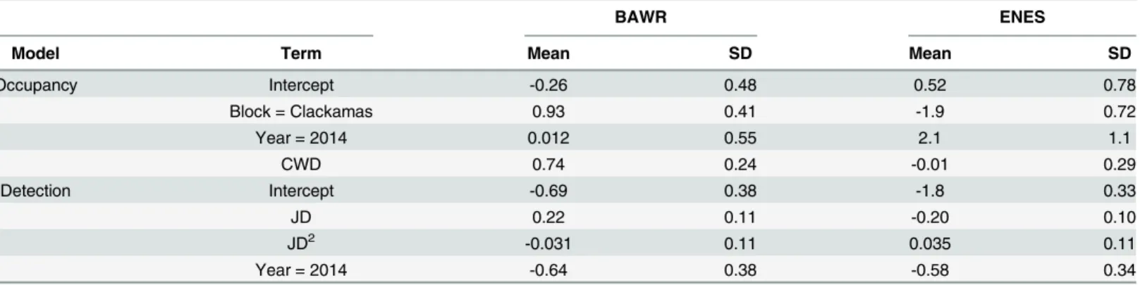
Evaluating Multi-Level Models to Test Occupancy State Responses of Plethodontid Salamanders.
Texto
Imagem
Documentos relacionados
The probability of attending school four our group of interest in this region increased by 6.5 percentage points after the expansion of the Bolsa Família program in 2007 and
Esse número se explica pela variação do teor de alimentação da usina, em muitos momentos menor que o utilizado para o dimensionamento do circuito, assim como do uso das
Definidos os métodos, a seguir iremos descrever as etapas de elaboração do trabalho conjuntamente com os métodos utilizados. Depois da formulação da pergunta de
Overall, even thought the meat enterococci present several antibiotic resistances and produce biofilms, due to a low number of virulence factors and to the absence
A responsabilidade penal não se prende pela indemnização/reparação do dano. Pelo contrário, poderá implicar a sujeição do médico à imposição de uma pena. Não obstante, é
É o caso dos sedimentos recolhidos no Núcleo Arqueológico da Rua dos Correeiros (NARC), no Criptopórtico Romano de Lisboa e no Banco de Portugal/Museu do Dinheiro (Praça do
Este estudo teve como objetivo adaptar e testar um procedimento de modificação das meso-estratégias de aprendizagem, isto é, verificar se a indução da consciencialização
The most frequent prey were three intro- duced mammals (house mice Mus musculus, ship rats Rattus rattus and rabbits Sylvilagus sp.) and the thin-billed prion Pachyptila belcheri
