Quantum Atom Optics with Trapped Bose-Einstein Condensates
M. K. Olsen
Instituto de F´ısica da Universidade Federal Fluminense, Boa Viagem 24210-340, Niter ´oi, RJ, Brazil
Received on 19 April, 2004
Both Bose-Einstein condensates and optical fields are composed of bosons, so that the majority of the processes which have long been studied in quantum and nonlinear optics have equivalents in the field of Bose-Einsten condensation. However, due to the masses of the condensed atoms, the confining potentials and the huge collisional nonlinearities, the simpler theoretical approaches common to quantum optics can sometimes give misleading answers when applied to condensates. In this work we describe some of the areas where simplified treatments can be misleading, and compare and contrast the predictions of quantum many-body treatments with those of the single-mode type treatments which have been so successful in quantum optics.
1
Introduction
Quantum optics was possibly the first area of physics which allowed for simple investigations of many of the funda-mental mysteries and paradoxes of quantum mechanics [1]. These investigations, both theoretical and experimental, were facilitated by the invention of the laser and the Fabry-Perot cavity and also by the fact that photons are essenti-ally non-interacting in vacuum. The laser can provide a bright source of well stabilised coherent light which is the starting point for many quantum optics experiments, while Fabry-Perot cavities select a small number of resonant mo-des which can then interact with a nonlinear medium to pro-duce light with nonclassical properties. The use of coherent states, the small number of modes which need to be taken into consideration, and the fact that any interaction is effec-tively only with the nonlinear medium all combine to sim-plify theoretical analyses. Even though the electromagnetic field is composed of many photons, an approximate theore-tical approach not much more complicated than that used in single-particle quantum mechanics often gives valid predic-tions.
When we wish to consider trapped Bose-Einstein con-densates (BEC), in principle there exist several ways to the-oretically model the dynamics of interacting condensates, but in practice we find that our options are somewhat li-mited. A full and exact treatment requires a description in terms of quantum fields, but as the resulting functional Heisenberg equations of motion are highly nonlinear, this approach is impracticable. An equivalent option, the quan-tum master equation, is totally impractical as the dimension of the required Hilbert space is far beyond the capacities of any computer. Assuming non-vanishing expectation va-lues for the field operators in the Heisenberg equations leads to the mean-field approach of the Gross-Pitaevskii equation (GPE) [2, 3], which, even though it is derived using quan-tum statistical considerations, cannot describe the effect of these on the dynamics. Worse, for systems of interacting
fields, the GPE has been shown to give misleading predic-tions in some parameter regimes [4, 5]. An alternative ap-proach which can say something about the quantum features is path-integral Monte Carlo [6], but this method is only re-ally practical for calculating ground state properties and not dynamical evolution. Other recent developments have been the use of stochastic wave functions [7] to solve N-boson time-dependent problems, and a stochastic GPE, developed from the quantum kinetic master equation [8]. We note here that all these approaches are truly in the realms of many-body theory and hence more complicated than the methods normally used in quantum optics. In this work we will give several examples where an oversimplified theoretical appro-ach, even though such approaches have enjoyed great suc-cess in quantum optics, can be shown to give misleading results.
2
Theoretical descriptions
2.1
An intracavity electromagnetic field
A single-mode non-interacting electromagnetic field can be described by a simple harmonic oscillator Hamiltonian,
Hf ree=~ωaˆ†ˆa, (1) whereˆais the well-known bosonic annihilation operator. If we wish to confine this mode inside an optical cavity, we must add pumping and damping terms,
Hpump = i~£ǫaˆ†−ǫ∗ˆa¤,
Hbath = ˆaΓˆ†+ ˆa†Γˆ, (2)
of Heisenberg equations for the intracavity field, in the rota-ting wave approximation [1],
d
dtˆa = ǫ−γˆa, d
dtˆa
† = ǫ∗
−γˆa†, (3)
whereγrepresents the cavity loss rate. Of course, a pumped cavity is not a particularly interesting system, so we may wish to include the interaction with an intracavity nonlinear medium, so as to produce nonclassical states of light. With the inclusion of this interaction, the equations do not gene-rally become much more complicated. We may also remem-ber that it is difficult to make measurements on the intraca-vity field, so that we will need to relate the field inside the cavity to that outside, which may be measured. This is easily done by using a set of input-output relations [9]. The main reasons that these have a simple form are that we can con-sider a small number of modes and the fact that photons are massless, so that once they leave the cavity, they are gone forever. The latter fact allows for the use of the Born and Markov approximations.
2.2
A trapped condensate
One of the simplest possible condensate systems, from an experimental and theoretical point of view, is a single spe-cies trapped Bose-Einstein condensate, in some ways ana-logous to the intracavity electromagnetic field described above. There have been relatively few attempts to treat the full quantum dynamics of this simple system, and it is so-metimes claimed that no computational approach is feasi-ble [10], due to the large size of the many-body Hilbert space. The first published attempt to dynamically model this system as a spatially dependent field, while rigorously in-cluding the quantum features, was by Steelet al.[11], who developed functional positive-P [12] and Wigner [13] repre-sentations for a trapped one-dimensional condensate, which were then used to calculate quantities such as the first order coherence properties.
By comparison with the simplicity of Eq. 3, a quantum calculation of the evolution of the BEC field operator is a formidable task, a direct route using a number state basis not being a realistic option due to the enormous size of the Hil-bert space. However, the phase-space techniques of quan-tum optics may be generalised to provide a complete des-cription of the condensate field operator. The key to this approach is the representation of the density operator using phase-space quasi-probability functions. We will now ou-tline the derivation of the equations resulting from the use of a functional positive-P representation.
A one-dimensional system can be considered by assu-ming a highly anisotropic harmonic trap with the longitu-dinal and radial trap frequencies (ωz andωr respectively) satisfyingλ = ωz/ωr ≪ 1. This corresponds to a cigar-shaped trap such as has commonly been used in experi-ments [14, 15]. The operator is then assumed to factorise so that we may write the one-dimensional longitudinal Hei-senberg field operator as
ˆ Ψ(x) =
³mωr π~
´1/2
exp
µ
−mωrr
2
2~
¶
ˆ
φ(z, t), (4)
wheremis the atomic mass. Adopting harmonic oscillator units in the axial direction witha0=
p
~/(mωz),τ =ωzt,
x=z/a0andψˆ(x, τ) = √a0φˆ(z, t), the one-dimensional
second-quantised Hamiltonian is (dropping the spatial de-pendence for notational convenience)
ˆ
H =
Z ∞ −∞
dxψˆ†Kψˆ+Γ 2
Z ∞ −∞
dxψˆ†ψˆ†ψˆψ,ˆ (5)
whereKis the linear operator
K=−1
2
d2 dx2 +
1 2x
2
−µ, (6)
µis the scaled chemical potential, and Γ = 2a/(λa0) is
the scaled nonlinear constant withathe s-wave scattering length.
The positive-P field equations may be obtained by intro-ducing the functionalP-distribution [16, 17]
P({ψ, ψ∗}, τ) = ρ(a)({ψ,ˆ ψˆ†}, τ)¯¯ ¯ˆ
ψ→ψ,ψˆ†→ψ∗ (7) whereρ(a) denotes the density operatorρ(τ)antinormally
ordered with respect to the field-operators ψ,ˆ ψˆ† in the Schr¨odinger picture. Putting the master equation obtained from the Hamiltonian (5) into antinormal order, and using the following functional analogues of the operator corres-pondences [18],
ˆ
ψρ ↔ ψP(ψ),
ˆ
ψ†ρ ↔
µ
ψ∗−δψδ
¶ P(ψ),
ρψˆ ↔
µ
ψ−δψδ∗ ¶
P(ψ),
ρψˆ† ↔ ψ∗P(ψ). (8)
one finds the functional Fokker-Planck equation,
⌋
∂P ∂τ =
Z ∞ −∞
dx ½
−δψδ(x)£
−i¡
Kψ(x) + Γ|ψ(x)|2ψ(x)¢¤
+Γ 2
δ2
δψ2(x)iψ
2(x)¾P+
The diffusion matrix of this equation is not positive-definite and so there is no straightforward mapping onto a single sto-chastic differential equation [18]. A positive-P representa-tion must be used, doubling the phase space with the map-ping
ψ(x, t) → ψ1(x, t),
ψ∗(x, t)
→ ψ∗
2(x, t), (10)
whereψ1(x, t) andψ2(x, t) are independent fields. Note
that sometimes the notation ψ+(x, t) is used instead of
ψ∗2(x, t), to denote the c-number field that corresponds to
ˆ
ψ†. We now obtain a positive-definite diffusion matrix and finally derive the pair of Itˆo stochastic differential equations,
⌋
i∂τψ1(x, τ) = Kψ1(x, τ) + Γψ∗2(x, τ)ψ21(x, τ) +
√
iΓψ1(x, τ)η1(x, τ),
i∂τψ2(x, τ) = Kψ2(x, τ) + Γψ∗1(x, τ)ψ22(x, τ) +
√
iΓψ2(x, τ)η2(x, τ), (11)
⌈
where the noise sourcesη1 andη2 are real, Gaussian and
delta-correlated in time and space, with the correlations, ηi(x, τ)ηj(x′, τ′) =δijδ(x−x′)δ(τ−τ′). (12) This set of coupled equations can then, in principle, be nu-merically integrated on a spatial lattice and averaged over a large number of trajectories to calculate any desired opera-tor moments. In practice, the numerical integration presents severe difficulties, although some progress has been made toward overcoming these [19, 20, 21, 22, 23]. We readily see that even the simplest method which can hope to give a complete description of a trapped condensate is much more complicated than the equations used to describe an intraca-vity electromagnetic field. If we were to add the equivalents of the pumping and damping terms as in the optical case, the situation would become even more complicated. For example, although we can model the laser pumping of an optical cavity in a very simple manner, the equivalent with the condensate is possibly evaporative cooling of a cloud of thermal atoms, which again needs a sophisticated theoretical treatment [24].
3
Quantum state of a trapped
con-densate
Another operational difference between quantum optics and BEC lies in the ease which with quantum states, usually re-presented by the appropriate Wigner function, can be found. When we wish to numerically integrate stochastic differen-tial equations to investigate the quantum dynamics of a gi-ven system, the initial conditions used can be very impor-tant. Generally in quantum optics, the laser which drives the system is accurately represented as a coherent state, whereas the quantum states of the interacting modes come naturally from the dynamics. However, for some quantum optical pro-cesses it has been shown that different initial states can result in quite different dynamics [25, 26]. As these processes have equivalents with BEC, we may assume that the initial state
of the trapped BEC should also be important in theoretical investigations.
In quantum optics, some of the most utilised states are the coherent state, the Fock state and the thermal state. The coherent state gives a good description of a well-stabilised laser operating above threshold, as well as for the field of a cavity pumped by such a laser. The Fock state, which has a fixed number of quanta, arises naturally when we consider the decay of a single excited atom, for example. The thermal state describes the radiation emitted by black-bodies. While other states are important, they usually arise because of the dynamics of a system and are not important as an initial con-dition in physically realistic calculations.
On the other hand, the quantum state of a trapped con-densate is almost certainly none of the above, although Fock and coherent states often appear as candidates in the litera-ture. The coherent state appeals because of the coherence properties exhibited [14, 27, 28], but has the problem of a largish uncertainty in number, which is conceptually diffi-cult to understand as atoms are not created or destroyed at typical temperatures. We should also remember that a cohe-rent state is cohecohe-rent to all orders, not just to first order as demonstrated by amplitude interference experiments. The Fock state is superficially an appealing choice, but as the condensate is in contact with an environment, particles can be added or removed. This state also has the problem that it has no defined phase. As the nonlinearity due to s-wave collisions between condensed atoms is equivalent to a Kerr interaction, we may expect to find that the actual state is none of the above. Several candidates have been offered in the literature, all making various levels of approximation. An early calculation [29] predicted an amplitude eigenstate, while a subsequent, more rigorous calculation [30], predic-ted a sheared Wigner function which approximapredic-ted a num-ber squeezed state. More recent attempts, using the Hartree approximation, found a Q-function which suggests both am-plitude quadrature and number squeezing [31] and a func-tion expressed in terms of generalised coherent states [32].
Wig-ner (or other pseudo-probability function) distribution is to solve the appropriate Fokker-Planck equation. With a trap-ped BEC, this is complicated by the fact that the equation for the Wigner function has third-order derivatives, so that the usual methods cannot be used [11]. Even after discar-ding these terms, the task is still not simple, as the equa-tion has both spatial and temporal dependence, is highly nonlinear, and contains kinetic energy and potential terms. Although the Hamiltonian exhibits some similarities to that of the Kerr amplifier, this latter system can be treated as zero-dimensional whereas this treatment is somewhat dubi-ous for a trapped BEC. It seems that the actual Wigner func-tion, once found, may prove to be spatially dependent as well as depending on the field variables. It is even possible that it may not be separable in terms of its different argu-ments, which would lead to a much more complicated func-tion than any of those proposed to date. That the calculafunc-tion or measurement of this Wigner function may be important has been shown in a series of articles which show that the process of photoassociation to form a molecular condensate exhibits dynamics which can depend on the actual initial quantum state [33, 34, 35, 36]. We will return to this subject in later sections.
4
Input-output relations
In quantum optics, the interaction of light with a nonlinear medium within a cavity is a common way of fabricating non-classical states of the electromagnetic field. As measure-ments are made on the field outside the cavity, we need a means of theoretically relating the fields within the cavity to those outside. Using the Born and Markov approxima-tions, Collett and Gardiner (see also Yurke [37]) developed the well-known input-output relations [9], which can be sim-ply written as
ˆ
aOU T(t) + ˆaIN(t) = p
2γˆa(t), (13) which is a boundary condition relating each of the far-field amplitudes outside the cavity to the internal cavity field. γ represents the cavity loss-rate. This relationship is easily transformed into frequency space, allowing for the simple calculation of output spectra. It can also provide, once me-asurements are made on the output fields, a simple way to calculate the field statistics inside the cavity.
The Born and Markov approximations which were used in the development of Eq. 13 have a restricted validity when we deal with trapped and outcoupled atomic systems as in, for example, Bose-Einstein condensates. The basic reason for this is that any atoms outcoupled from a trap tend to remain in the boundary region much longer than photons, which, being massless, exit at the speed of light. This me-ans that there is a finite time during which the atoms remain in this region, still being able to interact with the trapped state. Hence the first and second Markov approximations are not valid because the system now has a finite memory and the outcoupling does not happen instantaneously.
For-malisms to cope with general output coupling of trapped bo-sonic atoms have been developed [38, 39, 40, 41, 42, 43], allowing calculations to be made in the regime where the Markov approximation does not hold. These methods allow, for example, the calculation of the energy spectrum of the steady state output flux of a hypothetical continuous wave atom laser. It has also been shown in which regions of opera-tion the Markov approximaopera-tion may be valid, demonstrating that non-Markovian damping can lead to markedly different behaviours.
4.1
Non-Markovian output coupling
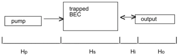
Following the approach of Hope et al. [42], we model a one-dimensional atom laser by separating it into three dis-tinct physical regions and an interaction region, as shown in Fig. 1. Starting from the left, we have the pump reservoir, coupled to the trap by an irreversible process, described by the HamiltonianHp. We do not specify a physical mecha-nism for the pump, but do state that it is not directly coupled to the output modes and is close enough to being a continu-ous process that we can consider the whole atom laser to be operating in the stationary regime.
>
< >
pump
trapped BEC
output
|______________|______________|____|_________|
Hp Hs Hi Ho
Figure 1. Schematic of a continuously pumped and outcoupled BEC, showing the approximate spatial regions of validity of each part of the Hamiltonian.
The lasing mode is a condensate contained in an atomic trap with large enough energy spacing to be considered as effectively operating in the single-mode regime. In order to simplify the treatment, we will ignore collisional interac-tions between the trapped atoms. This means that we can approximately describe the lasing mode by bosonic annihi-lation and creation operatorsaˆandˆa† and the Hamiltonian
Hs. The external output field consists of atoms in a different electronic or magnetic state to the lasing mode atoms, so that it is no longer trapped by the potential. The output modes are described by the bosonic field operatorsψˆ(x)andψˆ†(x) and the HamiltonianHo. The coupling between the lasing mode and the output field is described by the Hamiltonian
Hi, so that the total Hamiltonian is written
Htot=Hp+Hs+Hi+Ho, (14)
with
Hs = ~ω0aˆ†a,ˆ (15)
Hi = i~
Z ∞ −∞
dx³κ(x, t) ˆψ(x)ˆa†−κ∗(x, t) ˆψ†(x)ˆa´,
whereκ(x, t)represents the form of coupling between the condensate and the output field, andω0 represents the
fre-quency of the lasing mode. Note that, without atom-atom interactions, ω0 does not depend on the mode occupation.
As the pump does not couple directly to the external modes, the following commutation relationships hold
£
Ho,H(s,p)
¤
=hHo,aˆ(†) i
=hH(s,p),ψˆ(†)
i
= 0. (17)
Hopeet al.[42] have shown how it is possible to go to
the Heisenberg picture, resulting in the general input-output relationship for this system,
ˆ
ψH(x, t) = ˆψI(x, t)− Z t
t0
ds F(x, t, s)ˆaH(s), (18)
whereψˆH(x, t)andˆaH(t)are the Heisenberg operators cor-responding toψˆ(x)andˆa, and
ˆ
ψI(x, t) =eiH0(t−t0)/ ~ˆ
ψ(x, t0)e−iH0(t−t0)/
~
. (19) The memory function,F, is proportional to aδ-function in time in the Markovian case, giving the well known input-output relationships of quantum optics. More generally, it is
written
F(x, t, s) =
Z
dy κ∗(y, s)hψˆ
I(x, t),ψˆ†I(y, s) i
=
Z
dy κ∗(y, s)G(x, t, y, s), (20)
whereG(x, t, y, s)is the Green’s function propagator due to the output Hamiltonian,Ho, only. Eq. 20 allows us, in prin-cipal, to calculate any observables of the output field, provi-ded that we know the appropriate Green’s function and the history ofaˆH(s). We should also note here that, in the stati-onary regime,F(x, t, s)is actually a function of(x, t−s).
4.2
Inverting the relation
In an actual experimental situation, it would be more com-mon to perform measurements on the output of the atom la-ser, as it is this which is accessible. Hence we wish to invert the relationship (18) and thus find observables in the output which can be mapped onto properties of the lasing mode. Noticing that the integral in (18) is of the convolution type, we can use Laplace Transforms to find a formal solution as follows
⌋
LhψˆH(x, t) i
=LhψˆI(x, t) i
− L[F(x, t−u)]× L[ˆaH(u)], (21)
so that
L[ˆaH(u)] =
LhψˆI(x, t) i
− LhψˆH(x, t) i
L[F(x, t−u)] , (22)
and
ˆ
aH(u) =L−1
LhψˆI(x, t) i
− LhψˆH(x, t) i
L[F(x, t−u)]
. (23)
⌈
We can immediately see that, in the Markovian case this reduces to the usual quantum optical relationship, as the La-place Transform of the memory function is a constant. In the more general situation, we know the Green’s function propagator for free space with and without gravity [44]. In position space, the shape of the coupling is defined by the spatial wavefunction of the trapped state multiplied by the shape of the outcoupling device, which in the case of Ra-man outcoupling [45, 46], would be overlapping twin laser
beams. Making the simplifying assumptions that no net mo-mentum kick is given to the atoms and that the coupling is Gaussian in form,
κ(x, t) =√γ µ2σ2
k π
¶1/4
e−(σkx)2
, (24)
where~σkis the momentum width of the coupling andγthe
strength, the Green’s function propagator in the presence of gravity is found as
⌋
G(x, t, y, u) =
s
1
4πiλ(t−u)×exp
µi(x
−y)2
4λ(t−u)−
ig(t−u)(x+y) 4λ −
ig2(t
−u)3
48λ ¶
whereλ=~/2M. Using (20), the memory function is found as
F(x, t, u) =
µ
2
π
¶1/4r γσ k
1−4iσkλ∆t
×exp
µ
−∆tg(∆t
2g+ 6x) +i(∆t4g2+ 12∆t2gx
−12x2)λσ2
k
12λ(i+ 4∆tλσ2
k)
¶
, (26)
where∆t=t−u.
⌈
Settingg = 0gives the memory function for coupling into free space, which decays as 1/√tin the long time li-mit. This can be understood because, in the absence of a repulsive force or gravity, there is nothing to remove atoms from the region of the trap except for the spreading of the wavepacket. This happens on a time scale so long that it becomes difficult to decide at what time an atom has actu-ally left the interaction region and can no longer be coupled back into the trapped condensate, resulting in a bound state. This is, of course, not the normal case with photons, which leave the region at the speed of light. In practice this me-ans that to obtain full information about the lasing mode at
a particular time, we would have to make measurements of the output over an infinite time. Fortunately, in a real atom laser the atoms will be repelled from the trap at least by gra-vity, and perhaps also by a repulsive potential, although the atoms will still leave at far less than the speed of light.
4.3
Intensity measurements
The obvious and simplest measurement to make on the out-put field is an intensity measurement, that isψˆ†H(t) ˆψH(t), which can be made by atom counting techniques. From (18), we see that this can be expressed as
⌋
ˆ
ψ†H(t) ˆψH(t) = ·
ˆ
ψI†(t)− Z t
t0
du F∗(x, t−u)ˆa†H(u) ¸
×
·
ˆ
ψI(t)− Z t
t0
du′F(x, t−u′)ˆaH(u′) ¸
= ψˆI†(t) ˆψI(t)−ψˆ†I(t)× Z t
t0
du′F(x, t−u′)ˆaH(u′)−ψˆI(t)× Z t
t0
du F∗(x, t−u)ˆa†H(u)
+
Z t
t0
du F∗(x, t−u)ˆa†H(u)×
Z t
t0
du′ F(x, t−u′)ˆaH(u′). (27)
We find that this expression simplifies on taking expectation values,
hψˆH†(t) ˆψH(t)i=h Z t
t0
du F∗(x, t
−u)ˆa†H(u)
Z t
t0
du′F(x, t
−u′)ˆa
H(u′)i, (28)
⌈
but is still not easily inverted to give information about
hˆa†HaˆHi.
It is instructive to follow the same procedure for the optical case, beginning with a measurement of
ˆ
a†OU T(t)ˆaOU T(t). Using Eq. 13 and taking expectation va-lues, we may immediately write
hˆa†aˆ
i= 1
2γ ³
hˆa†INˆaINi+haˆ†OU TaˆOU Ti ´
, (29)
so that knowledge of the pumping and measurement of the output intensity tells us instantly the intensity inside the ca-vity.
4.4
Two-time correlation function
hψˆ†H(u) ˆψH(t)i= Z t
t0
dt′′ Z u
t0
dt′F∗(u−t′)hˆa†H(t′)ˆaH(t′′)iF(t−t′′), (30)
⌈
which is an equation relating the two-time correlation func-tions of the lasing mode and the output. Assuming stationa-rity, that is thathˆa†H(t+τ)ˆaH(t)iis independent oft, where u=t+τ, and also that the output is on an almost linear part of the dispersion curve (Note that, physically, this may be a difficult condition to fulfil, due to the quadratic dispersion of massive particles), we can take Fourier transforms to find a relationship between the power spectrum of the lasing mode and the power spectrum of the output,
Φψ(ν) =|F(ν)|2Φa(ν), (31) whereΦψ(ν)andΦa(ν)are the Fourier transforms of the two-time correlation functions of the output and lasing mode respectively, andF(ν)is the transform of the memory func-tion. Eq.(31) is then trivially rearranged to give the power spectrum inside the trap as a function of what is measured at the output,
Φa(ν) = Φψ(ν)/|F(ν)|2. (32) This quantity can then be inverse Fourier transformed to give us the two-time correlation function and hence a measure of the first order coherence of the trapped state. In the limiting case where the coupling tends to Markovian, F(ν)is flat, meaning that the correlation time inside and outside the trap will be equal, as in the optical case. In general, however, be-cause of the facts that the dispersion curve is not linear and the coupling is not Markovian, we see that the atomic case is more complicated.
We can also start with the relationship between the out-put energy flux and the two-time correlation function of the lasing mode [42]
dhˆc† pˆcpi
dt = 2|κ(p)|
2ReµZ t 0
du e−iωp(t−u)hˆa†(t)ˆa(u)i ¶
,
(33) which assumes that the output field was vacuum att = 0. In the above,ˆcpis the annihilation operator associated with the energy eigenstate of the output mode with position wa-vefunctionup(x)and energy~ωp, so that
κ(p, t) =
Z
dx up(x)κ(x, t). (34)
In the case where the only term in the output Hamiltonian is the kinetic energy, the eigenstates are the momentum ei-genstates so thatκ(p, t)is simply the Fourier transform of κ(x, t). In the more realistic case, with gravity, the eigens-tates are Airy functions with an energy-dependent displace-ment,
up(x) =NAi ·
β(x−~mgωp)
¸
, (35)
whereNis a constant of normalisation and the length scale is given byβ = (2m2g/~2)1/3. In this caseκ(p, t)can be
calculated numerically. We again see that the inversion of Eq. 33 to give knowledge of the internal atomic correlation function is much more difficult than in the optical case.
5
Raman superchemistry:
coupled
atomic and molecular condensates
5.1
Truncated Wigner approach
We will follow the treatment given in Refs. [33, 34] and show how a truncated Wigner representation can be used to model the dynamics of interacting atomic and molecu-lar condensates. We consider that the initial atomic con-densate is trapped such that one of the frequencies (ω0) is
much smaller than the other two, leading to a cigar
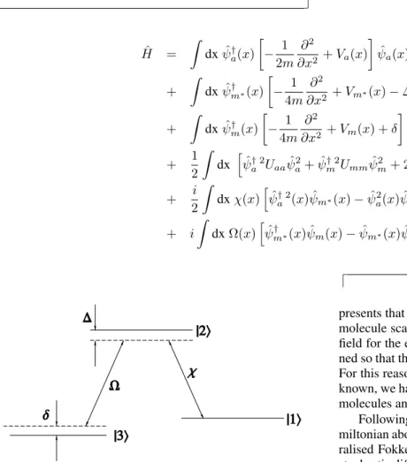
sha-ped condensate which may be approximated as one dimen-sional. We consider here a two laser Raman photoassocia-tion scheme [50, 4, 5] where the excited molecular field will be adiabatically eliminated. The three different atomic and molecular fields with the laser couplings and detunings are shown schematically in Fig. 2, with the process being des-cribed by the functional Hamiltonian (note that we use units such that~= 1)
⌋
ˆ
H =
Z
dxψˆ†a(x) ·
−21m ∂
2
∂x2+Va(x)
¸
ˆ
ψa(x)
+
Z
dxψˆ†m∗(x) ·
−41m ∂
2
∂x2 +Vm∗(x)−∆
¸
ˆ
ψm∗(x)
+
Z
dxψˆ†m(x) ·
−41m ∂
2
∂x2+Vm(x) +δ
¸
ˆ
ψm(x)
+ 1 2
Z
dx hψˆ†a2Uaaψˆa2+ ˆψ†m2Ummψˆ2m+ 2 ˆψ†aψˆm† Uamψˆaψˆm i
+ i 2
Z
dxχ(x)hψˆa†2(x) ˆψm∗(x)−ψˆa2(x) ˆψm†∗(x) i
+ i Z
dxΩ(x)hψˆm†∗(x) ˆψm(x)−ψˆm∗(x) ˆψm† (x) i
, (36)
⌈
d D
c W
|3ñ
|1ñ |2ñ
Figure 2. Energy level schematic of the coupled atomic and mo-lecular fields. |1irepresents the condensed atoms,|2ithe excited molecules, and|3ithe condensed ground state molecules. The
Ra-man laser coupling strengths are represented byχandΩ, with∆
representing the detuning from the excited molecular band andδ
representing the Raman detuning.
where mis the atomic mass, ψˆa(x)is the atomic field an-nihilation operator, ψˆm∗(x)is the excited molecular field annihilation operator, andψˆm(x)is the ground state mole-cular field annihilation operator. The Rabi frequency of the transition between atoms and excited molecules is represen-ted byχ(x)andΩ(x)is the Rabi frequency of the transition between excited and ground state molecules. In principle, these could also be time dependent. The bare detunings,∆
and δ, are as shown in Fig. 2. The trapping potentials are represented byVa (atoms),Vm(molecules) andVm∗ (exci-ted molecules). In the standard s-waveδ-function approxi-mation,Uaais the atom-atom interaction strength,Umm
re-presents that between molecules, andUamrepresents atom-molecule scattering. Note that we are considering only one field for the excited molecules as the lasers should be detu-ned so that their population will remain as small as possible. For this reason, and also because the strengths are not at all known, we have ignored spontaneous breakup of the excited molecules and any collisional interactions involving them.
Following the usual route [11, 18], we may map the Ha-miltonian above onto a master equation and this onto a gene-ralised Fokker-Planck equation. As stated above, although stochastic difference equations can be found which are equi-valent to the generalised Fokker-Planck equation, they are difficult to use. After discarding the third-order derivati-ves, which are assumed to be small, we may map the resul-ting Fokker-Planck equation onto three coupled differential equations forψj(j =a, m, m∗), which are now the com-plex variables of the Wigner representation. Although the neglect of the third-order derivatives may be thought of as an uncontrolled approximation, it is an approximation that has previously given good results in many systems, especi-ally when we only wish to calculate intensities. We note here that for a previous treatment of photoassociation using the positive-P representation [4], the truncated Wigner re-presentation gives almost identical predictions for the ato-mic and molecular numbers.
mea-sured in units ofω−01and space in units of
p
~/mω0, and
considering the laser couplings as spatially constant across
the trap, we find (for details see Ref. [34])
⌋
idψa
dt = −
∂2ψ
a
∂x2 +Va(x)ψa+
³
Uaa′ |ψa|2+Uam|ψm|2 ´
ψa+iκψa∗ψm
idψm
dt = −
1 2
∂2ψ
m
∂x2 +Vm(x)ψm+
³
Umm|ψm|2+Uam|ψa|2−δ ′´
ψm− i
2κψ
2
a, (37)
⌈
whereUaa′ =Uaa+χ2/2∆, and
κ = Ωχ
∆ ,
δ′ = δ+Umm−2Uaa− Uam
2 + Ω2
∆. (38)
The detuning from the Raman resonance is now represen-ted byδ′, which we will assume to be zero in our treatment. Note that we ignore interactions with any atoms of the ther-mal cloud which is usually found along with the conden-sed portion, as we are assuming that the condensate actu-ally is at zero Kelvin. In all our investigations we will use Uam =−1.5U
′
aa,Umm= 2U ′
aa,κ= 1,δ ′
= 0, and a mo-lecular trapping potential twice that of the harmonic atomic potential.
It must be stressed here that, although these equations have the form of coupled equations of the Gross-Pitaevskii type, they are not equations for the order parameter, the mean-fields, or for what are commonly called the macrosco-pic wavefunctions. They are equations for the complex va-riables of the Wigner representation of the two coupled con-densates and these variables are in fact stochastic, with the initial conditions obeying a probability distribution. There are also differences in the self and cross interaction terms, which come purely from the Wigner distribution and which cause a shift in the Raman detuning. There are basically two advantages to using the truncated Wigner representa-tion. Firstly, it allows for stable and rapid integration of the condensate equations when compared to the positive-P re-presentation and, secondly, it allows for simple modelling of many initial quantum states.
As a harmonic trapping potential is most commonly used in theoretical investigations of trapped condensates, we consider this case here. For purposes of comparison, we also numerically integrate the GPE type equations, which give semiclassical results with the quantum statistics playing no part in the time evolution. We emphasise here that the GPE solutions are not really physically relevant where they disa-gree with the quantum predictions, as it is impossible to turn off the quantum noise. What we find is that the spatial de-pendence of the trapped condensates plays an important role in the process, with the coupling rates at different densities being different. For the parameters used, this causes an inte-resting structure to emerge, with spatial sidebands forming
in the distributions. Over the times shown here, the kinetic energy of the condensates has little effect, with an averaging of the results of integration of spatially separate single-mode equations at each spatial point giving virtually identical pre-dictions, both spatially and for the total particle numbers. This is not the case for longer interaction times, where the atoms have time to move around due to both the trapping potential and the s-wave scattering processes.
To model the initial quantum states of the condensates, each of the 512 points in the spatial grid is given an ini-tial value on each trajectory, chosen from the Wigner dis-tribution for the appropriate state. A coherent state is mo-delled by taking the (real) ground state GPE solution for the nth spatial point and adding real and imaginary num-bers drawn from a normal Gaussian distribution, giving ψa(xn) =ψaGP(xn) +.5(η1(xn) +iη2(xn))/√∆x, where
∆xis the spacing of the numerical grid. It is easily verified that the trajectory average will be|ψGP(xn)|2+ 1/2∆xat each point, with 1/2∆x needing to be subtracted at each point once the trajectory averaging has taken place. A mi-nimum uncertainty squeezed state is modelled by adding .5(η1(xn)e−r+iη2(xn)er)/
√
∆xat each point, where r is the squeezing parameter. A sheared state, typical of Kerr nonlinearities, as in Dunningham et al. [30], is simulated by transforming the added squeezed state noise by a fac-torexp(iqη3(xn)), whereqis the shearing factor. The real noise terms have the correlations
ηj(xn) = 0, ηi(xm)ηj(xn) =δmnδij. (39) Numerical checks of single-mode distributions produced using these methods show that they give the expected values for average numbers and quadrature variances. In our simu-lations for squeezed states, we use values ofr=±log 0.5, while for the sheared state we usedq= 0.005, which give results similar to the Wigner function shown in Dunningham
et al. [30]. We also investigate a more extreme shearing
field always begins as a coherent vacuum, withψm(xn) = .5(η4(xn)+iη5(xn))/√∆xon each trajectory, with the ran-dom variables defined as in Eq. 39.
0 0.05 0.1 0.15 0.2 0.25 0.3 0.35 0.2
0.4 0.6 0.8 1 1.2 1.4 1.6 1.8
2x 10
4
t(units of ω0−1)
Na
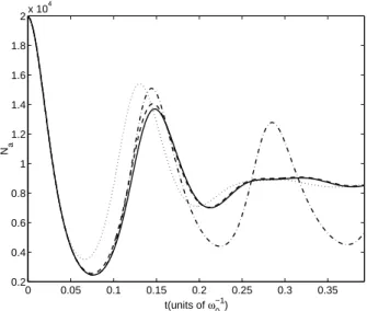
Figure 3. Atomic population predictions in the harmonic trap, up to
t=π/8. The dash-dotted line is from the GPE approach, the solid line is for an initial coherent state, the dashed line is the slightly sheared state and the dotted line is the crescent state.
In Fig. 3 we show the mean atom numbers, defined as Na= ∆x
X
k ³
|ψa(xk)|2−1/2∆x ´
, (40)
where klabels the points on the numerical grid. What we see is that when we use an initial coherent state in the Wig-ner equations, we do not find the dramatic differences from the GPE predictions for the first atomic revival as reported previously [4, 5]. The reason is simply that we are wor-king with different parameters, with the ratio betweenκand the strength of the nonlinear interactions being important in this regard. This was previously demonstrated to be the case in travelling wave second harmonic generation, with which, although it is not as rich a system as coupled condensates, a useful analogy can be made [52]. What we do see is that the oscillations predicted by Heinzenet al.[50] do not persist after the first atomic revival, once the quantum noise is ta-ken into account. This feature is not due to interactions with thermal atoms, as in G´oralet al.[53], as there are no ther-mal atoms present in our zero temperature treatment. Nor is it due merely to an averaging over different conversion rates at different positions within the condensates, as this avera-ging effect is also present in the GPE treatment. It is due to the quantum nature of the matter fields, cannot be represen-ted by classical treatments, and is intrinsic to the process of photoassociation.
An initial atomic state with the same degree of ampli-tude squeezing and shearing as calculated in Ref. [30] also does not lead to vastly different dynamics from the initial coherent state, the difference between the two being almost
negligible. However, a dramatic difference in the early dy-namics occurs when we consider the initialcrescentstate. The initial conversion to molecules for this state is not as complete and the first revival in the atomic population is earlier and more pronounced than for the other initial sta-tes. Interestingly enough, the longer time behaviour is al-most independent of the initial state, with the populations reaching a quasi-stationary state. Whether a later revival of the oscillations is present or not is difficult to predict using our methods, as the computational time required becomes prohibitive. However, we consider it unlikely as the system of interacting atomic and molecular condensates is probably too complicated to find the collapses and revivals predicted in, for example, the Jaynes-Cummings model of quantum optics [54].
The differences come in the first minimum of the atomic population and the subsequent revival and are readily explai-ned by the degree of phase uncertainty in the initial state. It can be seen by examination of Eq. 37 that whether associ-ation or disassociassoci-ation is predominant will partially depend on the phase of the productsψ∗
aψmandψa2. As the crescent state has a larger phase uncertainty than the others conside-red, the photodisassociation process begins to dominate and the mean number of atoms begins to revive at an earlier time than for the other states.
5.2
The zero dimensional approach
The equivalent of the simple quantum optics approach to photoassociation would be to treat each of the interacting condensates as a single-mode, which can then be represen-ted by a single variable, without any spatial dependence. This approach has been used, in a classical mean-field ap-proximation [55], claiming that to reproduce the results for a condensate with spatial dependence, all one needs to do is to take the average of integrations for different points from the spatially dependent condensate. If the condensate did in fact obey the mean field equations this approach would actually give reasonable results for short times. For processes which take place over longer times, the kinetic energy has an effect and atoms and molecules can move around, changing the behaviour. However, after a short time, the mean-field ap-proach can give completely wrong predictions for the popu-lations, even when we begin with coherent states. This has previously seen in travelling wave second harmonic genera-tion [51, 52], but is possibly not as important in that system due to the small nonlinearities and short interaction times of available χ(2) materials. With photoassociation, however,
we do not have the same limits on interaction time. The pro-cess will continue as long as the Raman lasers are switched on and the condensate remains stable, which should be suf-ficient to produce a large number of the superchemistry type oscillations if the mean-field picture were correct.
coupled equations dα
dt = −i
¡
Uaa|α|2+Uam|β|2¢α+κα∗β dβ
dt = −i
³
Umm|β|2+Uam|α|2−δ ′´
β−κ
2α
2,
(41) whereαandβnow represent atomic and molecular amplitu-des, respectively. The other parameters are all as in Eq. 37. Note that the lack of potential and kinetic energy in this ap-proach means that, apart from the detuningδ′, these equati-ons are mathematically equivalent to those used in Ref. [52]. One important difference from the optical case, however, is that theUij self and cross interaction terms are very much larger than those likely to be found in any optical system.
0 0.05 0.1 0.15 0.2 0.25 0.3 0.35 0
500 1000 1500 2000 2500
t(units of ω0−1)
Na
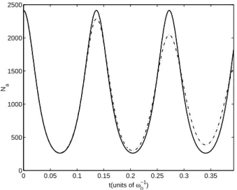
Figure 4. Zero dimensional predictions for the atomic population. The solid line represents the classical mean-field prediction, and the dash-dotted line is the stochastic prediction for an initial cohe-rent state, averaged over4.35×105
trajectories. In this case the other initial states do not show a noticeable difference from the coherent state.
We show the results for the atomic dynamics in Fig. 4, comparing the predictions of the truncated Wigner with an initial coherent state to those of the classical approach, both for an initial atom number equal to |ψa|2 at the centre of the densities used for the harmonic trap. Note here that this is not the same as the atomic number at the centre of the one-dimensional grid, which is∆x|ψa|2, but is the number which enters into the one dimensional equations. The re-sults for the other initial quantum states considered above are virtually indistinguishable from the coherent state. We find that the classical approach, which predicts regular peri-odic behaviour in this case, is reasonably accurate up to the second revival of atomic population, but then begins to differ from the quantum prediction. The quantum result shows a damping of the oscillations, due solely to the quantum noise. This serves to show that any averaging process using mean field solutions would eventually become an averaging over
erroneous values and could not be expected to lead to cor-rect predictions. We note also that it is very easy to find parameter regimes where the classical and quantum predic-tions are markedly different, even for early times. In this re-gard, the ratio betweenκand the s-wave interactions plays an important role, with the classical predictions becoming less accurate asκ/Uaais increased.
6
Fock state dynamics
In the absence of a complete solution for the Wigner func-tion, obtained without making various approximations, re-searchers have sometimes chosen to use Fock states. The Wigner function for the Fock state|Niis
WN(α, α∗) = 2
(−1)N
π exp(−2|α|
2)L
N(4|α|2), (42) where LN is the Laguerre polynomial of order N. This distribution is oscillatory and can obviously be either posi-tive or negaposi-tive, so cannot be easily simulated numerically. However, in the largeN regime Gardiner has made the ob-servation [8] that the cumulative distribution behaves very like a step function centered at|α|2 =N. This distribution
can then be approximated by a Gaussian with the right mo-ments, at least for the mean and variance. The appropriate distribution is
PN(n, θ) = r
2
πexp µ
−(n−N−1/2)
2
2(1/4)
¶
, (43)
where we have takenα=√neiθ, withθuniform on[0,2π). It can be shown that this approximation generates all mo-ments of (42), up to a correction of order1/N2, which is
negligible in the largeNregime.
To simulate this distribution numerically, consider the choice (using a single mode for simplicity)
αi=p+qηi, (44)
whereηi is a normal Gaussian random variable, andpand q are yet to be determined. As we are using a Gaussian approximation, it is sufficient to reproduce the first two mo-ments ofα2. (Note thatαis a real variable here, with the
phase distribution still to be added.) We need to reproduce α2=N+ 1/2andα4= (N+ 1/2)2+ 1/4. This gives us
p2+q2 = N+1 2,
p4+ 6p2q2+ 3q4 = (p2+q2)2+1
4, (45)
sinceη= 0,η2= 1, andη4= 3, which leads to
4p2q2+ 2q4= 1
4. (46)
Sincepwill be of the order of N andq will be less than one (q essentially gives the width of the Gaussian), we can neglect the term2q4to arrive at
q= 1
The relation for the mean then gives us p2+ 1
16p2 =N+
1
2, (48)
from which we choose the solution p=1
2
³
2N+ 1 + 2pN2+N´1/2. (49)
The αi thus chosen is then multiplied by the factor
exp(2iπξi), whereξis randomly chosen from the uniform distribution[0,1). Numerical tests with variables produced in this manner show that the required mean and variances are reproduced to a high degree of accuracy. Having now found a way to approximately reproduce the Wigner func-tion for an initial Fock state, we may integrate the Raman photoassociation equations (37) with this initial condition.
6.1
Fock state in zero dimensions
By comparison with a zero-dimensional quantum optics type approach, sometimes used to represent Raman photoas-sociation of atomic condensates [55], we can show that the quantum statistics become more important as the dimension increases. The zero dimensional system can be investigated with the coupled equations given above (41). We find that the results for the atomic dynamics of an initial Fock state are almost indistinguishable from those shown in Fig. 4 for an initial coherent state. We find that the classical mean-field approach, which predicts regular periodic behaviour in this case, is reasonably accurate up to the second oscillation, but then begins to differ from the quantum prediction. The quantum result shows a damping of the oscillations, due so-lely to the quantum noise. In a zero-dimensional analysis, the choices of initial quantum state used here do not cause major differences, with the initial coherent state and the ini-tial Fock exhibiting almost identical dynamics.
6.2
Fock state in one dimension
We will now return to a more realistic model which treats the interacting condensates as one dimensional. In Fig. 5 we show the results for the atomic numbers, using initial Fock, crescent and coherent states, all with the same initial mean numbers of atoms. Immediately obvious is that, for these parameters, the dynamics for the Fock state are completely different from the other two. Not only is the initial conver-sion rate less, but the degree of converconver-sion to molecules is much less, and there are no oscillations seen between atoms and molecules. The different dynamics of the Fock state cannot be ascribed to the initial spatial intensity correlation, g(2)(x, x)(see Ref. [34, 56]), as this between1
−1/N for a Fock state,1 for a coherent state, and1.04at the centre for the crescent state. As demonstrated above in Sec. 5, the more uncertainty in phase that a given state has by compari-son with a coherent state, the more difference we see in the dynamics. A Fock state, which exhibits the maximum pos-sible phase uncertainty of2π, is therefore expected to differ
most in its dynamics from the coherent state. That this phase uncertainty has a more pronounced effect in one dimension is because phase gradients are set up within the condensate on each trajectory, which means that the atoms will move around within the trap. Even though these movements may average out when we take the mean over the stochastic tra-jectories, they destroy the spatial coherence necessary to see oscillations.
0 0.01 0.02 0.03 0.04 0.05 0.06 0.07 0.08 0.09 0
0.2 0.4 0.6 0.8 1 1.2 1.4 1.6 1.8
2x 10
4
t (units of ω0−1) Na
Fock
coherent crescent
Figure 5. Atom number evolution for Fock, crescent and coherent initial states.
Compared with the zero dimensional predictions, the re-sults for the Fock state are quantitatively different. Although there is a difference for the coherent state, it is only quan-titative. This is a clear example of the importance of the underlying dimensionality, which has long been appreciated in critical phenomena and is now shown to play a role in the quantum dynamics of interacting atomic and molecular condensates. We see that the zero-dimensional predictions, which can be found analytically under certain approximati-ons, and have been used in, for example [57, 58] with initial Fock states, are far from the1D results. We note here that, while there are certain physical conditions to be fulfilled so that a trapped BEC may be effectively considered as one-dimensional (see, for example, Ref. [56]), we are not aware of any physical conditions which would allow for the zero-dimensional models sometimes used to investigate photoas-sociation.
7
Twin beams via photodissociation
7.1
Parametric downconversion
degree of quantum correlation between the produced low frequency photons. It can easily be shown theoretically that these twin photons are entangled and, in the nondegenerate case, allow for a demonstration of the Einstein-Podolsky-Rosen (EPR) paradox with continuous variables [59]. If we make the approximation that the pump field is undepleted, we can find analytical solutions. In the optical case, this is often a good approximation, as the conversion efficiency of commonly used nonlinear crystals can be of the order of1
in1013. We begin with the interaction Hamiltonian
H=i~χ³ˆa†1aˆ†2−ˆa1ˆa2´, (50)
where theaˆjare annihilation operators for the low frequency modes and the coupling constantχ is proportional to the nonlinearity of the medium and the pump amplitude. In this case we find solutions to the Heisenberg equations of motion as
ˆ
a1(t) = ˆa1(0) coshχt+ ˆa†2(0) sinhχt,
ˆ
a2(t) = ˆa2(0) coshχt+ ˆa†2(0) sinhχt, (51)
which, starting from vacuum, predict a number of photons in each mode
hnˆj(t)i= sinh2χt, (52) whereˆnj = ˆa†jˆaj. We thus see that the effect of this device is to amplify the vacuum in the two low-frequency modes. An obvious consequence of this system is that the following conservation law holds:
ˆ
n1(t)−nˆ2(t) = ˆn1(0)−nˆ2(0), (53)
which allows for a high degree of squeezing in the number difference.
What is more interesting for our purposes here is that the OPA also exhibits phase-dependent quantum correlati-ons which can be used to demcorrelati-onstrate entanglement and the EPR paradox. Using the fact that two-mode squeezing is predicted in the combined quadraturesYa+YbandXa−Xb, (whereXa = ˆa+ ˆa† andYa = −i(ˆa−ˆa†)) and the inse-parability criterion proposed by Duanet al.[60], it may be shown that entanglement is guaranteed provided that [61]
V(Ya+Yb) +V(Xa−Xb)<4. (54) With vacuum inputs, we may find analytical expressions for both these variances, as
V(Ya+Yb) =V(Xa−Xb) = 2e−χt, (55) showing that the degree of entanglement can, in principle, become perfect. In reality, the non-depleted pump approxi-mation will break down and the entanglement will be found to be maximal for some finite interaction time [62].
A demonstration of the EPR paradox using this system has been outlined in Refs. [59, 61]. Essentially, the quadra-ture operatorsXa,b andYa,b take the place of the position and momentum operators considered in the original treat-ment [63]. Basically, we can make linear estimates of the variances of two non-commuting quadratures, which, when multiplied together, seemingly violate the Heisenberg uncer-tainty principle. We define the inferred variances
Vinf(Xa) = V(Xa)−
[V(Xa, Xb)]2 V(Xb)
,
Vinf(Ya) = V(Ya)−
[V(Ya, Yb)]2 V(Yb) ,
(56)
whereV(A, B) =hABi−hAihBi. All the quantities above can be calculated analytically, giving
Vinf(Xa)Vinf(Ya) =
1
cosh22χt, (57) whereas the productV(Xa)V(Ya)≥1. Again, these analy-tical predictions lose their validity after a certain interaction time, as the undepleted pump approximation becomes unte-nable.
7.2
Molecular dissociation
We will now analyse the process of photodissociation of a molecular condensate to see how much physics can be ad-ded before the simple analyses of Sec. 7.1 lose their vali-dity. Poulsen and Mølmer [64] have used the positive-P re-presentation to predict squeezing in the number difference between two beams of dissociated atoms, considering the original molecular condensate as undepleted. The atomic state resulting from photo-dissociation is used as a squeezed input to the matter wave analog of a50/50beam splitter. The other input is a large conventional condensate of atoms in a different internal state, but with a well-defined relative phase. The squeezing in the particle number difference re-fers to the resulting two outputs of this atomic beam splitter. Kheruntsyan and Drummond have shown that, with the ap-propriate detunings on the Raman lasers, two spatially sepa-rated output beams can be produced directly from photodis-sociation, without the need for an atomic beamsplitter [65]. They predict a high degree of number squeezing between these beams. In both these analyses the full spatial problem was considered, but Ref. [65] also considered depletion of the molecular condensate.
We will outline here the treatment of Ref. [65], making various levels of approximation. The effective Hamiltonian for the atomic (Ψˆ1) and molecular (Ψˆ2) fields, taken for
ˆ
H = Hˆkin+ Z
dx
X
i
Vi(x) ˆΨ†iΨˆi+
1 2
X
i≥j
UijΨˆ†iΨˆ † jΨˆjΨˆi
−iχ(t)
2
h
eiωtΨˆ†2Ψˆ21−e−iωtΨˆ2Ψˆ†12
i¾
, (58)
⌈
with the commutation relations [ ˆΨi(x, t),Ψˆ†j(x′, t)] = δijδ(x−x′). HereHˆkinstands for the usual kinetic energy term,Vi(x)is the trapping potential (including internal ener-gies),U11 ≃4π~a1/(Am1)represents the atom-atom
scat-tering strength in one dimension, wherem1is the mass,a
is the three-dimensionalS-wave scattering length, andAis the confinement area in the transverse direction, with simi-lar results for the molecule-molecule and molecule-atom in-teractions. The term proportional toχ(t)describes a cohe-rent process of molecule-atom conversion via Raman photo-dissociation, whereχ(t)is the coupling constant related to the transition matrix elements and the amplitudes of the Ra-man lasers which have an overall frequency differenceω.
The atoms are assumed to be untrapped longitudinally (they may be in anm = 0magnetic sublevel) yet confined transversely (they may be in a transverse optical trap), so that the atomic field can effectively be treated as a free one-dimensional field, initially in a vacuum state. We neglect the atom-atom collisions since we restrict the coupling to short interaction times during which the atomic density remains small. The detuning∆ ≡ V1(0)−[V2(x0) +ω]/2, where
V2(x0) =V2(0) +U22n2(0), is proportional to the energy
mismatch between the atomic and molecular fields, withx0
the axial half-length in the Thomas-Fermi approximation. The absolute value of the detuning|∆|is chosen to be non-zero and much larger than the magnitude ofU12hΨˆ†2Ψˆ2iso
that the effect of atom-molecule s-wave scattering is also negligible. We now introduce characteristic length,d0, and
time scales,t0= 2m1d20/~, and transform to dimensionless
fields in rotating frames. Introducing a dimensionless detu-ningδ = ∆t0and couplingκ(t) = χ(t)t0/√d0, we may
write the Heisenberg equations of motion for the (dimensi-onless) field operators as,
∂ψˆ1(ξ, τ)
∂τ = i
∂2ψˆ 1
∂ξ2 −iδψˆ1+κψˆ2ψˆ
†
1,
∂ψˆ2(ξ, τ)
∂τ =
i
2
∂2ψˆ
∂ξ2 −iˆv2(ξ) ˆψ2−
1 2κψˆ
2 1. (59)
Note that we have introduced an effective potentialˆv2(ξ) =
[V2(ξd0)−V2(ξ0d0)]t0+uψˆ†2ψˆ2, whereu=U22t0/d0, for
notational simplicity.
In Ref. [65], the positive-P version of the above equati-ons was solved numerically to show that two spatially sepa-rated output atomic beams with a high degree of squeezing in the number difference could be created. In fact, for this
correlation, an accurate insight was provided by the analyti-cal solutions of single-mode type equations, as used above in Sec. 7.1. We will now move on to the phase-sensitive corre-lations required to show entanglement and the EPR paradox, demonstrating that the extrapolation from the simple equati-ons is no longer so straightforward. To gain some analytical insight, we first consider an idealised model corresponding to an undepleted and uniform molecular condensate at den-sityn2(0), that fills the entire space from−l/2tol/2, with
periodic boundary conditions. The atom-molecule coupling χ = χ0 is assumed to be constant during the whole
evo-lution time from0toτ. In a manner analogous to the un-depleted pump approximation, the molecular field can be absorbed into an effective gain constantg =κ0
p n2(0)d0
(whereκ0 = χ0t0/√d0), which we assume to be real and
positive. Solutions to the resulting linear equations for the atomic field are easily found in momentum space by expan-dingψˆ1(ξ, τ)in terms of single-mode bosonic annihilation
operators:ψˆ1(ξ, τ) =Pqˆaq(τ)eiqξ/√l, whereq=d0kis
a dimensionless momentum. The corresponding Heisenberg equations of motion are
dˆaq(τ)
dτ = −i
¡ q2+δ¢
ˆ
aq+gˆa†−q,
dˆa†−q(τ)
dτ = i
¡ q2+δ¢
ˆ
a†−q+gˆaq, (60) which simplifies the problem as the coupling is now between opposite momentum components only. The above equations have the solutions
ˆ
aq(τ) = Aq(τ)ˆaq(0) +Bq(τ)ˆa†−q(0),
ˆ
a†−q(τ) = Bq(τ)ˆaq(0) +A∗q(τ)ˆa †
−q(0), (61) where
Aq(τ) = cosh (gqτ)−iλqsinh (gqτ)/gq , Bq(τ) = gsinh (gqτ)/gq , (62) whileλq ≡q2+δ, andgq ≡(g2−λ2q)1/2.
of the atomic field, we can calculate any operator moments at timeτ. We will consider that all momentum components are initially in the vacuum stateaˆq(0)|0i= 0.
We now consider, following Ref. [59], the measurements that must be made to demonstrate the EPR paradox. It is re-adily seen that correlations exist between atomic quadratu-res of the beams with opposite momentum components. For example, a measurement ofXˆq(=aq+ ˆa†q)allows us to in-fer, with some error, the value ofXˆ−q, and vice-versa. The same holds for theYˆq(=−i(a−q−ˆa†−q)quadratures. This allows us to define, depending on which beam we measure, four inferred variances,
Vinf(Xq) = V(Xq)−
[V(Xq, X−q)]2 V(X−q)
,
Vinf(Yq) = V(Yq)−[V(Yq, Y−q)]
2
V(Y−q) ,
Vinf(X−q) = V(X−q)i −[V(Xq, X−q)]
2
V(Xq) ,
Vinf(Y−q) = V(Y−q)−[V(Yq, Y−q)]
2
hY2
qi
. (63)
As the products of the non-inferred variancesV(X±q)and V(Y±q)are bound by the Heisenberg uncertainty principal to be greater than or equal to one, the paradox exists for Vinf(X
q)Vinf(Yq) < 1 or Vinf(X−q)Vinf(Y−q) < 1. As an example demonstrating the paradox we consider the correlations between the momentum components q = |δ| andq =−|δ|corresponding to the perfect phase matching condition withλq= 0, whereδ <0. In this simple case we obtain
Vinf(Xq=|δ|)Vinf(Yq=|δ|) =
1 cosh2(2gτ),
Vinf(Xq=−|δ|)Vinf(Yq=−|δ|) =
1
cosh2(2gτ),(64)
which are identical to the OPA results of Eq. 57. As can be seen, this simple analysis shows an obvious demonstration of the EPR paradox.
It is extremely instructive to see what happens when we look at a more physical model. We return to the more re-alistic case as described by the full Hamiltonian of Eq. 58, which is mapped onto stochastic differential equations in the positive-P representation Including a term to describe possi-ble linear losses at a rateγresults in the equations:
⌋
∂ψ1
∂τ = i
∂2ψ 1
∂ξ2 −(γ+iδ)ψ1+κψ2ψ + 1 +
p κψ2η1,
∂ψ+1
∂τ = −i
∂2ψ+ 1
∂ξ2 −(γ−iδ)ψ + 1 +κψ
+ 2ψ+
p κψ2η+1,
∂ψ2
∂τ =
i
2
∂2ψ 2
∂ξ2 −iv(ξ, τ)ψ2−
κ
2ψ
2 1+
√
−iuψ2η2,
∂ψ+2
∂τ = −
i
2
∂2ψ+ 2
∂ξ2 +iv(ξ, τ)ψ + 2 −
κ
2ψ
+2 1 +
√
iuψ2+η2+ . (65)
⌈
Here ψi and ψ+i are complex stochastic fields correspon-ding respectively to the operators ψˆi and ψˆ†i, v(ξ, τ) =
[V2(ξd0)−V2(ξ0d0)]t0+uψ2ψ2+ represents the effective
potential, and ηi , η+i are four real independent delta-correlated Gaussian noise terms: hηi(ξ, τ)ηj(ξ′, τ′)i =
hηi+(ξ, τ)η+j(ξ′, τ′)
i=δijδ(ξ−ξ′)δ(τ−τ′).
We consider the molecules as initially being in a (real) coherent state, represented spatially by the Thomas-Fermi solution, assuming repulsive molecule-molecule interacti-ons. The time duration for the molecule-atom conversion is controlled via κ(τ) = κ0θ(τ1−τ), so thatκ(τ) = 0
for τ > τ1, where θ is the Heaviside function. Once the
dissociation is stopped, we continue the evolution of the re-sulting atomic field in free space to allow spatial separation of the modes with positive and negativeqvalues. What we find is that the product of the inferred variances for opposite
to demonstrate the EPR paradox with a realistic system, it seems that we will need a more sophisticated model than is provided by naively adopting the OPA equations to a spati-ally dependent condensate.
We can demonstrate the momentum mixing with a sim-ple model, with two momentum components at ±k, which are strongly correlated and coupled by an interaction g0.
We then add interactions with other components at±k±
∆k, with an adjustable parameter, g1, which regulates the
strength of the mode-mixing, represented here as a nearest neighbour type interaction in momentum space. In the un-depleted case we can write an appropriate interaction Ha-miltonian,
⌋
H = i~g0ha†
1a
†
4−a1a4+a†2a
†
5−a2a5+a†3a
†
6−a3a6
i
+i~g1ha†
1a
†
5−a1a5+a†2a
†
4−a2a4+a†2a
†
6−a2a6+a†3a
†
5−a3a5
i
. (66)
⌈
We will be interested in correlations between a2(−k)and
a5(k), with the other modes beinga1(−k−∆k), a3(−k+
∆k)anda4(k−∆k), a6(k+ ∆k). By adjustingg1, we can
change the strength of the mode-mixing interactions. The above Hamiltonian, being only quadratic in the ope-rators, has an exact mapping onto stochastic equations for the Wigner variables, giving
dα1
dt = −i∆α1+g0α ∗
4+g1α∗5,
dα2
dt = g1α ∗
4+g0α∗5+g1α6∗,
dα3
dt = i∆α3+g1α ∗
5+g0α∗6,
dα4
dt = −i∆α4+g0α ∗
1+g1α∗2,
dα5
dt = g1α ∗
1+g0α∗2+g1α3∗,
dα6
dt = i∆α6+g1α ∗
2+g0α∗3, (67)
where we have now included a detuning, ∆, which is equal to the momentum spacing between adjacent modes. The αi are the stochastic variables of the Wigner repre-sentation which probabilistically represent symmetrically-ordered operator products.
We now wish to calculate the inferred variances,
Vinf(X2) = V(X2)−
[V(X2, X5)]2
V(X5)
,
Vinf(Y2) = V(Y2)−
[V(Y2, Y5)]2
V(Y5) ,
(68)
and their equivalents forX5andY5, which will be equal due
to the symmetry of the equations. Integrating these equati-ons over104stochastic trajectories, with initial states being
the Wigner vacuum, gives the results shown in Fig. 6. In these results, we have set∆ = 184.1andg0 = 3.35×10³,
equal to the numerical values used in the full equations. The time axis is within the limits of validity of the undepleted
molecule approximation forg1 = 0, with less than1%
mo-lecular depletion. Overall, we see that the sensitivity to this mode-mixing is not linear, but that any non-zero amount of mode-mixing does act to degrade the correlations. By com-parison with full spatial results, we see that a realistic effect coupling for this model is probably aroundg1 = 0.75g0.
The fact that the products shown do not begin at exactly one is because of sampling error in the Wigner distribution, due to an averaging over a finite number of trajectories. We also note here that much is missing from this simple model, such as atom-atom, molecule-molecule and atom-molecule scat-tering, for example, but that it does show that a realistic spa-tial treatment of the trapped BEC is necessary if we wish to reproduce the physics of these EPR correlations.
0 0.5 1 1.5 2 2.5 3 3.5 4 0
0.2 0.4 0.6 0.8 1 1.2 1.4 1.6 1.8 2
g0t
V
inf(X)V inf(Y)
0.5g
0
0.75g0
Figure 6. Product of the inferred variances from the Wigner equa-tions, withg1 = 0g0, 0.25g00.5g0and0.75g0.
We can also look at the variances for the combined qua-dratures,X2−X5andY2+Y5, shown in Fig. 7, which
de-monstrate the degree of entanglement between modes2and