Growth and production of the copepod community in the southern area of the Humboldt Current System

(1)

BGD

12, 3057–3099, 2015

Growth and production of the copepod community

R. Escribano et al.

Title Page

Abstract Introduction

Conclusions References

Tables Figures

◭ ◮

Back Close

Full Screen / Esc

Printer-friendly Version Interactive Discussion

Discussion

P

a

per

|

Discussion

P

a

per

|

Discussion

P

a

per

|

Discussion

P

a

per

Biogeosciences Discuss., 12, 3057–3099, 2015 www.biogeosciences-discuss.net/12/3057/2015/ doi:10.5194/bgd-12-3057-2015

This discussion paper is/has been under review for the journal Biogeosciences (BG). Please refer to the corresponding final paper in BG if available.

Growth and production of the copepod

community in the southern area of the

Humboldt Current System

R. Escribano1,2, E. Bustos-Ríos1,2, P. Hidalgo1,2, and C. E. Morales1,2

1

Instituto Milenio de Oceanografía (IMO), Concepción, P.O. Box 160 C, Chile 2

Departamento de Oceanografía, Universidad de Concepción, Concepción, P.O. Box 160 C, Chile

Received: 17 December 2014 – Accepted: 15 January 2015 – Published: 10 February 2015

Correspondence to: R. Escribano (rescribano@udec.cl)

(2)

BGD

12, 3057–3099, 2015

R. Escribano et al.

Title Page

Tables Figures

◭ ◮

Back Close

Full Screen / Esc

Discussion

P

a

per

|

Discussion

P

a

per

|

Discussion

P

a

per

|

Discussion

P

a

per

|

Abstract

Zooplankton production is a critical issue for understanding marine ecosystem struc-ture and dynamics, however, its time-space variations are mostly unknown in most systems. In this study, estimates of copepod growth and production (CP) in the coastal upwelling and coastal transition zones off central-southern Chile (∼35–37◦S) were

5

obtained from annual cycles during a 3 year time series (2004, 2005, and 2006) at a fixed shelf station and from spring–summer surveys during the same years. C-specific growth rates (g) varied extensively among species and under variable environmental conditions; however,g values were not correlated to either near surface temperature or copepod size. Copepod biomass (CB) and CP were higher within the coastal

up-10

welling zone (<50 km) and both decreased substantially from 2004 to 2006. Annual CP ranged between 24 and 52 g C m−2year−1with a mean annualP/Bratio of 2.7. We estimated that CP could consume up to 60 % of the annual primary production (PP) in the upwelling zone but most of the time is around 8 %. Interannual changes in CB and CP values were associated with changes in the copepod community structure, the

15

dominance of large-sized forms replaced by small-sized species from 2004 to 2006. This change was accompanied by more persistent and time extended upwelling dur-ing the same seasonal period. Extended upwelldur-ing may have caused large losses of CB from the upwelling zone due to an increase in offshore advection of coastal plank-ton. On a larger scale, these results suggest that climate-related impacts of increasing

20

wind-driven upwelling in coastal upwelling systems may generate a negative trend in zooplankton biomass.

1 Introduction

Variability in biological production of lower trophic levels is a critical issue for under-standing the dynamics of marine ecosystems of the world ocean (Mann and Lazier,

25

(3)

BGD

12, 3057–3099, 2015

R. Escribano et al.

Title Page

Tables Figures

◭ ◮

Back Close

Full Screen / Esc

Discussion

P

a

per

|

Discussion

P

a

per

|

Discussion

P

a

per

|

Discussion

P

a

per

in capturing, retaining and transferring freshly produced phytoplankton-carbon toward higher levels (Poulet et al., 1995; Kimmerer et al., 2007). Despite this wide recogni-tion, there are no many studies targeting zooplankton secondary production and its time-space variability in the ocean, making difficult to assess the actual role of zoo-plankton in controlling or limiting biological production of high trophic levels, including

5

fish, mammals and seabird populations (Aebischer et al., 1990; Beaugrand et al., 2003; Castonguay et al., 2008). Zooplankton secondary production is the total biomass pro-duced by a population or community per unit of area or volume over a unit of time (Kimmerer et al., 2007), regardless the fate of such biomass (Winberg, 1971). There is, however, not a single and simple method to estimate zooplankton production and

10

growth rates but several approaches have been applied and di_fferent results obtained (Avila et al., 2012; Lin et al., 2013); even more, most of the traditionally applied meth-ods are logistically difficult to apply as to characterize time-space variations in these rates (Sastri et al., 2013; Mitra et al., 2014).

In the case of copepods, the dominant components of zooplankton biomass in the

15

oceans, there have been several attempts to develop theoretical and empirical relation-ships between zooplankton production and the factors known to a_ffect their growth. For instance, temperature has been widely reported as a fundamental factor influencing copepod growth (Huntley and Lopez, 1992; McLaren, 1995; Escribano et al., 2014), while body size should also be considered as a fundamental driver on the basis that

20

growth, as any other physiological rate, must be modulated by allometric effects (West et al., 1997). In fact, both variables have motivated the development of the metabolic theory of ecology (Brown et al., 2004) which proposes that animal growth is predictable from body size and environmental temperature. Meantime, other studies have provided evidence that food resources can often limit zooplankton growth (Hirst and Lampitt,

25

(4)

BGD

12, 3057–3099, 2015

R. Escribano et al.

Title Page

Tables Figures

◭ ◮

Back Close

Full Screen / Esc

Discussion

P

a

per

|

Discussion

P

a

per

|

Discussion

P

a

per

|

Discussion

P

a

per

|

particular condition or community but one of the critical problems for the calculation of secondary production is having reliable estimates of in situ growth rates of the species comprising the bulk of the zooplankton biomass in a given region or area. As mentioned above, weight or C-specific growth rate (g) has been related to temperature, food con-ditions, and body size, but in most cases direct estimates ofgshow no relation or very

5

weak relationships with these factors (e.g. Lonsdale and Levinton, 1985; Chisholm and Roff, 1990; Hutchings et al., 1995).

The Humboldt Current System (HCS) is one of the Eastern Boundary Currents (EBC’s) known by its high biological productivity (Mann and Lazier, 1991), attributed usually to the high levels of primary production in the coastal zone (>10 g C m−2d−1)

10

sustained by wind-driven upwelling (Daneri et al., 2000; Montero et al., 2007). Cope-pods and euphausiids dominate the zooplankton biomass in the HCS off Chile (Es-cribano et al., 2007; Riquelme-Bugueño et al., 2012), however, very few studies on zooplankton production are available. Escribano and McLaren (1999) estimated sec-ondary production for the dominant copepodCalanus chilensisin the upwelling region

15

offnorthern Chile, and Vargas et al. (2009) estimated growth and production of three copepod species in the upwelling region o_ffcentral-southern Chile during an annual cy-cle. Riquelme-Bugueño et al. (2013) described the population dynamics and biomass production of the Humboldt Current “Krill”,Euphausia mucronata, for the same region. Although euphausiids may occasionally become very abundant in this region, the bulk

20

of zooplankton biomass in the coastal upwelling zone is dominated by copepods, and, more specifically, by small-sized (<2 mm) copepods (Escribano et al., 2007). Hence, the latter may well reflect the dynamics of the whole zooplankton biomass and pro-duction in the southern area of the Humboldt Current (Hugget et al., 2009). A group of about 10 copepod species comprises >90 % of the total numerical abundance

25

(5)

genera-BGD

12, 3057–3099, 2015

R. Escribano et al.

Title Page

Tables Figures

◭ ◮

Back Close

Full Screen / Esc

Discussion

P

a

per

|

Discussion

P

a

per

|

Discussion

P

a

per

|

Discussion

P

a

per

tions per year (Vargas et al., 2009). The cyclopoidsOithona similisand O. nana, and the poecilostomadoidsTriconia conifer, T. media, andCorycaeus typicusare also abun-dant (Hidalgo et al., 2010). Larger-sized (>2 mm) copepods are mainly represented by

Calanus chilensisin the northern region and Calanoides patagoniensisin the central-southern region (Hidalgo et al., 2010), and, occasionally, byRhyncalanus nasutusand

5

Eucalanaus spp., including E. inermis and E. glacialis (Castro et al., 1993; Hidalgo et al., 2010).

In this work, we first assessed growth rates of the dominant copepod species found in the coastal upwelling zone offcentral-southern Chile during the spring–summer pe-riod and under time-space variations in environmental conditions, including

tempera-10

ture and food resources, which allowed us to test the influence of copepod size and temperature on the C-specific growth rate (g). Secondly, we used a species-dependent

gvalue to calculate copepod biomass production and its time-space variability in the domain of the coastal upwelling and coastal transition zones, therby contributing to provide the first estimates of copepod community production in the Humboldt Current

15

and to understanding the factors causing time-space variability in copepod growth and production in this upwelling region.

2 Methods

2.1 Field studies

Copepod abundance estimates were obtained from a 3 years time series (2004–2005,

20

and 2006) at a fixed shelf station (Station 18,∼36.5◦S, ∼30 km from the coast), in-cluding monthly samplings, and from spring–summer surveys during the same years (Table 1), with stations located in the coastal and the coastal transition zones off central-southern Chile (35–39◦S; Fig. 1). In addition, wind data were obtained from a meteo-rological station (Fig. 1) since August 2004; speed and direction were measured every

25

(6)

BGD

12, 3057–3099, 2015

R. Escribano et al.

Title Page

Tables Figures

◭ ◮

Back Close

Full Screen / Esc

Discussion

P

a

per

|

Discussion

P

a

per

|

Discussion

P

a

per

|

Discussion

P

a

per

|

upwelling index:

τ=ρcdV|V| (1)

where τ=wind stress (kg s m−2), ρ=air density assumed as 1.2 kg m−3, cd=is an empirical constant₌0.0013, andV is the alongshore component of the wind in m s−1. Station 18 represents an oceanographic time series study launched by COPAS

Cen-5

ter (Escribano and Schneider, 2007) and it includes rosette CTDO deployments and plankton monitoring. Zooplankton sampling was performed on a monthly basis using a 1 m2 Tucker Trawl net equipped with 200 µm mesh size nets and a calibrated flow-meter; deployments from 80 m depth to surface provided integrated samples; details on sampling procedures are provided in Escribano et al. (2007).

10

Space variations in copepod abundance were assessed through spring–summer, oceanographic cruises covering the upwelling and the coastal transition zones (up to 180 km from the coast). The sampling grid varied slightly from year to year (Fig. 1 and Table 1). During these spatial surveys, similar procedures as those of the time series study were applied to obtain hydrographic data and zooplankton samples. For

15

zooplankton sampling, however, the Tucker Trawl equipment was deployed down to 200 m depth, or near bottom in shallower stations. CTDO casts and bottle samples were obtained at each station, together with chlorophylla(Chla) estimations in at least 7–9 depths in the upper 100 m depth at each station.

2.2 Copepod biomass and growth

20

Copepod biomass is needed to calculate secondary production. Biomass estimates for each species we obtained from mean weight estimates and length–weight relationships (REFS). For this purpose, we first calculated the mean body size of all copepodid stages for each species (Table 2) and then we applied a length-weight regression to estimate mean weight (as dry weight). Length-weight regressions were obtained from

25

(7)

BGD

12, 3057–3099, 2015

R. Escribano et al.

Title Page

Tables Figures

◭ ◮

Back Close

Full Screen / Esc

Discussion

P

a

per

|

Discussion

P

a

per

|

Discussion

P

a

per

|

Discussion

P

a

per

estimated as:

B_i =

N

X

i=1

(w_in_i)0.4 (2)

whereBi is the species-i biomass (µg C m−

3

),wi andni are the mean dry weight (µg)

and abundance (number m−3) of thei-species and 0.4 is the conversion factor to µg C from dry weight (Escribano et al., 2007).

5

Several studies carried out in the last few years in the upwelling zone offChile have provided estimates of in situ growth rates (g) of copepods for different copepodid stages and species (Table 2). Most of these studies have applied the molting rate method, by using artificial cohorts (review in Harris et al., 2000). We made use of this set of estimates to examine the influence of temperature and copepod size on growth and,

10

from that, we attempted to develop an empirical equation to predict in situ g’s from these variables for each of the dominant species in the samples.

2.3 Data analyses

Copepod production for each species was estimated from their biomass andgvalues as to obtain total production, such that:

15

CP₌

N

X

i=1

(Bigi) (3)

where CP=total copepod production (mg C m−3d−1), B_i=as defined above and

g_i=C-specific growth rate (d−1) for eachi-species.

CP was calculated for each sampling station during the spatial cruises and each of the monthly samplings during the time series. CP integrated values in the water column

20

(8)

BGD

12, 3057–3099, 2015

R. Escribano et al.

Title Page

Tables Figures

◭ ◮

Back Close

Full Screen / Esc

Discussion

P

a

per

|

Discussion

P

a

per

|

Discussion

P

a

per

|

Discussion

P

a

per

|

annual production/biomass ratio (P/B) was also obtained. Oceanographic data were all processed to construct spatial contours (cruises) and temporal contours (time series). Similar procedures were applied to copepod abundance, biomass and production as to identify space–time patterns.

Relationships betweeng and temperature and body size were tested by linear and

5

non-linear regression methods, and goodness-of-fit was tested by correlation, the de-termination index and ANOVA. Meantime, eventual associations among copepod vari-ables and oceanographic factors were assessed by General Linear Models (GLM) and Stepwise Multiple Regression applied on log-transformed data on copepod abundance, biomass and CP.

10

3 Results

3.1 Oceanographic conditions

The three spatial surveys were carried out during the period of coastal wind-driven up-welling, as evidenced by the surface distributions of temperature and salinity (Fig. 2). During the 2004 cruise, recently upwelled waters (<13◦C and >34 psu) were found

15

in the northern and central areas in the coastal band; the offshore extension of these waters in the central area indicates that there may be one or more (sub) mesoscale eddies located in that area. Coastal upwelling activity was also observed during the 2005 cruise but colder waters (<12◦C) with higher salinities were restricted to the nearshore, except for lower salinity water offand within the Arauco Gulf (∼37◦S). In

20

the 2006 cruise, upwelling was concentrated in the northern area and restricted to a narrow coastal band (<40 km from shore) so that, in general, waters were less saline compared to 2004 and 2005. Upwelling conditions during the surveys were also evi-dent from the surface distributions of dissolved oxygen (DO) and Chla concentration (Fig. 3). Remarkable differences in DO distribution among the cruises were found. In

25

(9)

BGD

12, 3057–3099, 2015

R. Escribano et al.

Title Page

Tables Figures

◭ ◮

Back Close

Full Screen / Esc

Discussion

P

a

per

|

Discussion

P

a

per

|

Discussion

P

a

per

|

Discussion

P

a

per

the central area which showed lower oxygenation (<4 mL L−1) in a zonal band where higher salinities were detected, and an oversaturated zone (>6 mL L−1) in the north-ern part, coinciding also with higher salinities (Fig. 2), together with high Chlalevels (>10 mg m−3). During the 2005 cruise, oxygenation levels were lower (<5 mL L−1) in the entire region and more so in the coastal zone where higher salinities were

ob-5

served, except in area around the Arauco Gulf. Chla distribution was similar to that in 2004, with high levels in the nearshore area in the northern and central areas. In 2006, highly oxygenated conditions (>6 mL L−1) prevailed in most of study region, except in the coastal band. High levels of DO coincided with greater Chlaconcentrations in the entire region compared to 2004 and 2005 (Fig. 3, lower panel).

10

During the time series study, daily-integrated data of wind stress, and their monthly means, were estimated for the period from August 2004 to May 2007. Since data for the time series were available from January 2004 through December 2006, wind data were divided into two periods having the same number of days and same months as to assess whether upwelling conditions had changed during these periods. There was

15

a clear seasonality in upwelling favorable winds (τ’s with positive values), such that potential for upwelling initiated in August and remained favorable until April–May of each year, while downwelling conditions prevailed in the winter period between June to early August (Fig. 4). In the first period of the time series (2004–2005), there were 205 days favorable for upwelling (τ >0) and downwelling was intense and persistent

20

throughout early winter (May 2005) to late winter (August 2005). In the second period (2006–2007), there were 255 days favorable for upwelling and downwelling conditions in winter were less intense and persisted for a shorter time (∼115 days) compared to the first period (Fig. 4).

At Station 18, the three annual cycles based on monthly sampling clearly revealed

25

(10)

pre-BGD

12, 3057–3099, 2015

R. Escribano et al.

Title Page

Tables Figures

◭ ◮

Back Close

Full Screen / Esc

Discussion

P

a

per

|

Discussion

P

a

per

|

Discussion

P

a

per

|

Discussion

P

a

per

|

vail below 30 m depth upon the non-upwelling period in winter (Fig. 5a). Upwelling also brings to the surface layer high salinity water (>34 psu) whereas a layer of freshwa-ters appears in winter such that higher stratification is generated due to increased river runoff(Fig. 5b). During upwelling conditions, oxygen-deficient conditions dominate in shallow subsurface waters (<20 m depth) due to the shallowness of the oxygen

min-5

imum zone (OMZ) in the region. By contrast, the water column becomes oxygenated down to near bottom during non-upwelling (Fig. 5c). The annual bloom of phytoplank-ton starts in early spring (September–October), coinciding with the setup of upwelling, and Chlaremains high until the end of summer in most cases.

3.2 Copepod growth rates

10

Several studies in the last few years have estimatedgfor dominant copepod species from the Chilean upwelling zone; most of them are based on laboratory studies sim-ulating a variety of temperature and food conditions in the field and, therefore, their results represent reliable estimates ofg. A summary of estimates ofgfor different de-velopmental stages and species, including body size of tested individuals, is provided

15

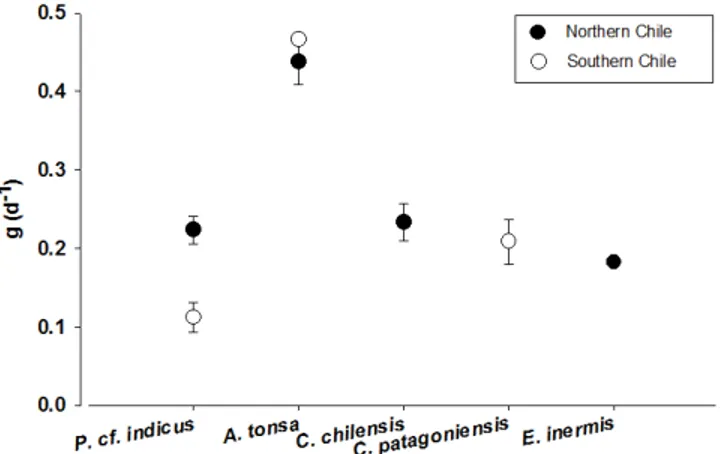
in Table 2. Because of potential allometric effects on growth rate, we attempted to de-velop a size-dependent model to predictgas a function of body size (Fig. 6a). Although an apparent decrease in g with size is observed, no significant correlation between these two variables was found (P >0.05) after testing with different lineal (GLM) and non-linear models.

20

Since temperature has been established as an important factor a_ffecting growth rate of copepods (Huntley and Lopez 1992; Gillooly et al., 2001), it was thought that this variable could be a suitable predictor of g under variable environmental conditions. For all the availablegestimates, we tested the influence of in situ simulated tempera-ture; also, no significant effects were found (P >0.05) after lineal (GLM) and non-lineal

25

(11)

BGD

12, 3057–3099, 2015

R. Escribano et al.

Title Page

Tables Figures

◭ ◮

Back Close

Full Screen / Esc

Discussion

P

a

per

|

Discussion

P

a

per

|

Discussion

P

a

per

|

Discussion

P

a

per

production rates (Fig. 7). For those species in which no estimates ofgwere available, a grand mean of copepod growth rate was applied (mean±SD: 0.27±0.133 d−1).

3.3 Copepod biomass and production

Copepod abundance (N), biomass (CB) and production (CP) were estimated as annual means for both the spatial surveys and the time series (Table 3). In both cases, strong

5

variability inN, CB and CP was observed (coefficient of variation: 25–50 %). Spatial variability ofN relates to a greater aggregation of copepods in the upwelling zone and decreasing values towards the offshore (Fig. 8). The highest values of CB and CP were also concentrated in the upwelling zone although there was a strong variation from year to year, with lower values in 2004 (Fig. 9).

10

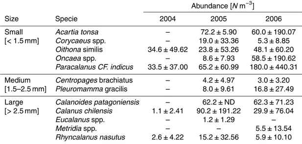
Copepod species in three size categories, in according to their total length: small (<1.5 mm), medium (1.5–2.5 mm) and large (>2.5 mm), varied substantially from year to year (Table 4). Small-sized species increased in abundance from 2004 to 2006, whereas large-size species tended to decreased in the same years. The distribution of these 3 size categories also varied from one year to another (Fig. 10). Medium

15

size species were absent in 2004 and large-sized species were more abundant in the upwelling zone, while small-sized species became more abundant in 2005 and even more so in 2006 and concentrated in the upwelling zone.

From the time series at Station 18, no seasonal pattern or trend in copepod abun-dance was detected (Fig. 11a), as was the case for CB and CP (Fig. 11b); in both

20

cases, lower values were detected during 2006. Integrated annual CP at station 18 was 52.2, 32.8 and 24.0 g C m−2y−1 for 2004, 2005 and 2006, respectively. From an-nual means of monthly integrated biomasses, the anan-nualP :Bratios obtained were 2.5, 2.8 and 2.9 for 2004, 2005 and 2006, respectively. The dailyP :B ratio was, on aver-age, 0.24. The variance of CB for each year, estimated from the coefficient of variation,

25

(12)

BGD

12, 3057–3099, 2015

R. Escribano et al.

Title Page

Tables Figures

◭ ◮

Back Close

Full Screen / Esc

Discussion

P

a

per

|

Discussion

P

a

per

|

Discussion

P

a

per

|

Discussion

P

a

per

|

3.4 Environmental effects on biomass and production

Using the data from the spatial surveys, a stepwise multiple regression was applied to test the effect of year of sampling and oceanographic conditions on N, CB and CP. Copepod data were previously log-transformed and a 1-step function was applied. Significant differences among years inNand CP were found. Chlacorrelated positively

5

withN, whereas Chla, DO and OMZ depth correlated with CP (Table 5).

For the time series data, we used cross-correlations between copepod variables and oceanographic conditions (including temperature, Chla, DO, and OMZ depth) to test for eventual associations. Although all the oceanographic factors showed a seasonal pattern, characterized by upwelling and downwelling periods (Fig. 5), copepod

abun-10

dance, biomass and production did not but their monthly fluctuations are rather random (Fig. 11). Therefore, it was not surprising that no significant correlations (P >0.05) be-tweenN, CB and CP and derived oceanographic variables were found.

4 Discussion

The oceanographic conditions observed during this study are those expected from

15

previous studies in the upwelling zone (Strub et al., 1998; Hidalgo et al., 2012; Morales and Anabalón, 2012) and the coastal transition zone (Letelier et al., 2009). The spatial surveys, conducted during spring–summer conditions, show that upwelling conditions prevailed in a coastal band along the study are of about 50 km width, coinciding with the isobath of 200 m (shown in Fig. 1). These conditions are characterized by colder,

20

more saline and less oxygenated water. This coastal band constitutes the main habitat of a few dominant copepods species (Hidalgo et al., 2010), and as evidenced by their aggregation over the shelf (Fig. 8). The same species are, however, present in the coastal transition zone although in lower abundances, probably as a result of their offshore transport by mesoscale eddies (Morales et al., 2010), which are originated in

25

(13)

BGD

12, 3057–3099, 2015

R. Escribano et al.

Title Page

Tables Figures

◭ ◮

Back Close

Full Screen / Esc

Discussion

P

a

per

|

Discussion

P

a

per

|

Discussion

P

a

per

|

Discussion

P

a

per

Most of the copepod production (CP) takes place in the coastal upwelling zone, where food resources (as represented by Chla) are also concentrated.

If most CP occurs in the upwelling zone, Station 18 is therefore a suitable location to assess its temporal variability. Oceanographic variability there also clearly shows the upwelling signal (Sobarzo et al., 2007a; Montero et al., 2007; Morales and

An-5

abalón, 2012). At this location, the copepod community has been well studied (Es-cribano et al., 2007; Hidalgo and Es(Es-cribano, 2007), and even though some seasonal signals in abundance and age-structure of some species have been described (Castro et al., 1993; Hidalgo and Escribano, 2007), most populations can grow and reproduce throughout the year (Vargas et al., 2009; Escribano et al., 2014), suggesting that CP

10

is a process taking place year-round. It should be noted, however, that a significant correlation of copepod abundance and CP with Chladoes not necessarily means that CB is being controlled by phytoplankton biomass. CP also correlates significantly with low oxygen and a shallow OMZ which, the same as for higher Chla levels, coincide in the zone were greater CP occurs. The question on whether CP can be controlled

15

or limited by phytoplankton biomass cannot be answered from the spatial survey just because of spatial correlation. On the other hand, no correlation between Chl a and CP was found in the time series data, and copepod abundance, CB and CP appeared uncoupled to the seasonal pattern of Chla.

In our approach to estimate copepod production, the use of species-dependent

20

growth rates may be justified on the basis thatg is a physiological rate controlled by two processes, development rate (DR) and tissue accumulation. In fact, estimating DR is the most widely used approach to assess growth rate of copepods. DR has been widely studied in copepods (McLaren and Leonard, 1995; Heinle, 1969) and it is con-sidered a species-dependent attribute (Heinle, 1969; Atkinson, 1994). Nevertheless,

25

within speciesgmay strongly vary (Runge and Ro_ff, 2000) and the use of a constantg

(14)

BGD

12, 3057–3099, 2015

R. Escribano et al.

Title Page

Tables Figures

◭ ◮

Back Close

Full Screen / Esc

Discussion

P

a

per

|

Discussion

P

a

per

|

Discussion

P

a

per

|

Discussion

P

a

per

|

body size (Hirst and Sheader, 1997), although size effects may not be reflected at the intra-specific level but among species (Banse, 1982; Peters, 1983). Temperature on the other hand may strongly affectgby accelerating or retarding the development of cope-pods (McLaren, 1995). It is therefore expected thatg would correlate positively with temperature. From our oceanographic surveys, however, temperature seems to vary

5

in a rather narrow range (∼11.5–13.5◦C) in the mixing layer of the upwelling zone, where dominant copepods aggregate and whose diel vertical distribution is restricted by a shallow (<50 m) OMZ during the upwelling period (Escribano et al., 2009). Thus, because of its little variation within the upwelling zone of central/southern Chile, tem-perature may not be the key factor controllingg.

10

It is not important to consider that copepod production represents only a fraction of total secondary production for the upwelling zone. Our estimate of CP does not consider molt and egg production of copepods either, but only somatic biomass pro-duction. With respect to the bulk of zooplankton, in the time series at Station 18 total zooplankton biomass (TZB) was available for the same period, as published in

Escrib-15

ano et al. (2007). TZB shows more variability than copepod biomass (CB) (Fig. 12a) and, on occasions, CB may account up to 96 % of TZB although on average our esti-mate of CB represents nearly 40 % of TZB. Meantime, monthly means of primary pro-duction (g C m−2d−1) in the same upwelling zone (Daneri et al., 2000) indicates that copepod production could take up to 60 % of the C being produced by phytoplankton

20

(winter 2004) although the mean conversion of PP into CP was about 8 % (Fig. 12b). This figure is in according with global mean estimates of the effect of mesozooplankton on PP (as the percent PP consumed per day: mode 6 %, mean 23 %) and decreases exponentially with increasing productivity (Calbet, 2001).

Recently, Escribano et al. (2012) and Pino-Pinuer et al. (2014) have described a

neg-25

(15)

BGD

12, 3057–3099, 2015

R. Escribano et al.

Title Page

Tables Figures

◭ ◮

Back Close

Full Screen / Esc

Discussion

P

a

per

|

Discussion

P

a

per

|

Discussion

P

a

per

|

Discussion

P

a

per

study, CB and CP significantly decreased from 2004 to 2006 at Station 18, although this trend was unclear in the spatial surveys. Copepods are strongly subjected to offshore advection during upwelling (Peterson, 1998; Keister et al., 2009; Morales et al., 2010). When examining the spatial patterns of oceanographic conditions, it appears that in 2005 and 2006 the upwelling focuses were concentrated near the location of Station

5

18, judging by low oxygen water in that area (Fig. 3), as compared to 2004 when the upwelling focus was located farther from the nearshore. It is therefore likely that cope-pods populations were more subjected to offshore advection in 2005 and 2006.

Another possibility for lower biomass and production in 2005 and 2006 could be explained in terms of food-limitation for copepod growth, as suggested for other

sys-10

tems (e.g. Hirst and Lampitt, 1998). Nevertheless, we found no significant di_fferences in phytoplankton biomass (as food indicator) among the three years. Also, primary pro-duction (PP) estimated monthly at Station 18 during the same period, showed that the annual cycle of PP almost repeated every year (Montero et al., 2007). Furthermore, o_ff Central/southern Chile, copepods can sustain their reproduction and growth

through-15

out the year, despite the seasonal bloom of phytoplankton, by switching their diet from autotrophic preys to an omnivorous diet (Vargas et al., 2006). Therefore, it is unlikely that annual CP could be limited by food in this upwelling region.

Since copepods mostly concentrate in the Ekman layer (<50 m) during upwelling, more o_ffshore advection, upon increased upwelling, can cause biomass loss from the

20

coastal zone. In fact, from our analysis of wind data we showed that favorable condi-tions for upwelling were more persistent (lasted longer) during the second part of the time series and hence promoting more export of CB to o_ffshore areas. Active upwelling also promotes formation of mesoscale intra-thermocline eddies (Hormazabal et al., 2013) which can also enhance plankton export from the upwelling zone.

25

(16)

consid-BGD

12, 3057–3099, 2015

R. Escribano et al.

Title Page

Tables Figures

◭ ◮

Back Close

Full Screen / Esc

Discussion

P

a

per

|

Discussion

P

a

per

|

Discussion

P

a

per

|

Discussion

P

a

per

|

ered as a C loss. Over an annual basis, we estimated how much of the C produced by phytoplankton is converted into CP and CB, and the annual deficit in CP that biomass loss can cause due to more advection driven by increased upwelling. The impact of greatly incremented upwelling is shown in Fig. 13, which illustrate how combined fac-tors and processes, such as upwelling conditions, CP, CB and primary production may

5

have interacted during the time series as to cause a reduction in copepod production in the upwelling zone. It is important to stress that upwelling intensity may not signif-icantly change from one year to another in average, but the length and continuity of the upwelling season can be the key process causing more biomass loss on an annual basis.

10

Acknowledgements. This work has been funded by the Chilean Funding for Science and Tech-nology (Fondecyt) Grant 113-0539 and IAI ANTARES Project. The time series study at Station 18 was funded by FONDAP COPAS Program of CONICYT of Chile. The Instituto Milenio de Oceanografía (IMO-Chile), funded by the Chilean Ministry of Economy, provided additional sup-port for data analyses, discussion and writing.

15

References

Aebischer, N. J., Coulson, J. C., and Colebrook, J. M.: Parallel long-term trends across four marine trophic levels and weather, Nature, 347, 753–755, 1990.

Arcos, D. F.: Copépodos Calanoideos de la Bahía de Concepción, Chile, Conocimiento Sis-temático y Variación Estacional, Gayana, 32, 1–43, 1975.

20

Atkinson, D.: Temperature and organism size: a biological law for ectotherms?, Adv. Ecol. Res., 25, 1–58, 1994.

Avila, T. R., de Souza Machado, A. A., and Bianchini, A.: Estimation of zooplankton secondary production in estuarine waters: comparison between the enzymatic (chitobiase) method and mathematical models using crustaceans, J. Exp. Mar. Biol. Ecol., 416–417, 144–152, 2012.

25

Beaugrand, G., Brander, K. M., Lindley, J. A., Souissi, S., and Reid, P. C.: Plankton effect on cod recruitment in the North Sea, Nature, 426, 661–664, 2003.

(17)

BGD

12, 3057–3099, 2015

R. Escribano et al.

Title Page

Tables Figures

◭ ◮

Back Close

Full Screen / Esc

Discussion

P

a

per

|

Discussion

P

a

per

|

Discussion

P

a

per

|

Discussion

P

a

per

Calbet, A.: Mesozooplankton grazing effect on primary production: a global comparative analy-sis in marine ecosystems, Limnol. Oceanogr., 46, 1824–1830, 2001.

Castro, L. R., Bernal, P. A., and Troncoso, V. A.: Coastal intrusion of copepods: mechanisms and consequences on the population biology ofRhincalanus nasutus, J. Plankton Res., 15, 501–515, 1993.

5

Chisholm, L. A. and Roff, J. C.: Size–weight relationships and biomass of tropical neritic cope-pods offKingston, Jamaica, Mar. Biol., 106, 71–77, 1990.

Daneri, G., Dellarossa, V., Quiñones, R., Jacob, B., Montero, P., and Ulloa, O.: Primary pro-duction and community respiration in the Humboldt Current System offChile and associated oceanic areas, Mar. Ecol.-Prog. Ser., 197, 41–49, 2000.

10

Escribano, R. and McLaren, I. A.: Production of Calanus chilensis in the upwelling area of Antofagasta, northern Chile, Mar. Ecol.-Prog. Ser., 177, 147–156, 1999.

Escribano, R. and Schneider, W.: The structure and functioning of the coastal upwelling system o_ffcentral/south of Chile, Progr. Oceanogr., 75, 343–346, 2007.

Escribano, R., Hidalgo, P., González, H. E., Giesecke, R., Riquelme-Bugueño, R., and

Man-15

ríquez, K.: Interannual and seasonal variability of metazooplankton in the Central/south up-welling region offChile, Prog. Oceanogr., 75, 470–485, 2007.

Escribano, R., Hidalgo, P., Fuentes, M., and Donoso, K.: Zooplankton time series in the coastal zone off Chile: variation in upwelling and responses of the copepod community, Prog. Oceanogr., 97–100, 174–186, 2012.

20

Escribano, R., Hidalgo, P., Valdés, V., and Frederick, L.: Temperature effects on development and reproduction of copepods in the Humboldt Current: the advantage of rapid growth, J. Plankton Res., 36, 104–116, 2014.

Finlay, K. and Roff, J. C.: Ontogenetic growth rate responses of temperate marine copepods to chlorophyll concentration and light, Mar. Ecol.-Prog. Ser., 313, 145–156, 2006.

25

Gillooly, J. F., Brown, J. H., West, G. B., Savage, V. M., and Charnov, E. L.: Effects of size and temperature on metabolic rate, Science, 293, 2248–2251, 2001.

Harris, R., Wiebe, P., Lenz, J., Skjoldal, H.-R., and Huntley, M. (Eds.): ICES Zooplankton Methodology Manual, Academic Press, London, 684 pp., 2000.

Hidalgo, P., Escribano, R., Vergara, O., Jorquera, E., Donoso, K., and Mendoza, P.: Patterns of

30

(18)

BGD

12, 3057–3099, 2015

R. Escribano et al.

Title Page

Tables Figures

◭ ◮

Back Close

Full Screen / Esc

Discussion

P

a

per

|

Discussion

P

a

per

|

Discussion

P

a

per

|

Discussion

P

a

per

|

Hirst, A. G. and Bunker, A. J.: Growth of marine planktonic copepods: global rates and patterns in relation to chlorophylla, temperature, and body weight, Limnol. Oceanogr., 48, 1988–2010, 2003.

Hirst, A. G. and Lampitt, R. S.: Towards a global model of in situ weight-specific growth in marine planktonic copepods, Mar. Biol., 132, 247–257, 1998.

5

Hirst, A. G. and Sheader, M.: Are in situ weight-specific growth rates body-size independent in marine planktonic copepods? A re-analysis of the global syntheses and a new empirical model, Mar. Ecol.-Prog. Ser., 154, 155–165, 1997.

Hopcroft, R. R., Clarke, C., and Chavez, F. P.: Copepod communities in Monterey Bay during the 1997–1999 El Niño and La Niña, Prog. Oceanogr., 54, 251–264, 2002.

10

Hormazabal, S., Combes, V., Morales, C. E., Correa-Ramirez, M. A., Di Lorenzo, E., and Nuñez, S.: Intrathermocline eddies in the coastal transition zone offcentral Chile (31–41S), J. Geophys. Res., 118, 1–11, 2013.

Huggett, J., Verheye, H., Escribano, R., and Fairweather, T.: Copepod biomass, size compo-sition and production in the Southern Benguela: spatio–temporal patterns of variation, and

15

comparison with other eastern boundary upwelling systems, Prog. Oceanogr., 83, 197–207, 2009.

Huntley, M. E. and Lopez, M. D. G.: Temperature-dependent production of marine copepods: a global synthesis, Am. Nat., 140, 201–242, 1992.

Hutchings, L., Verheye, H. M., Mitchell-Ines, B. A., Peterson, W. T., Huggett, J. A., and

Paint-20

ing, S. J.: Copepod production in the southern Benguela system, ICES J. Mar. Sci, 52, 439– 455, 1995.

Kimmerer, W. J., Hirst, A. G., Hopcroft, R. R., and McKinnon, A. D.: Estimating juvenile copepod growth rates: corrections, inter-comparisons and recommendations, Mar. Ecol.-Prog. Ser., 336, 187–202, 2007.

25

Letelier, J., Pizarro, O., and Nuñez, S.: Seasonal variability of coastal upwelling and the up-welling front offcentral Chile, J. Geophys. Res., 114, C12009, doi:10.1029/2008JC005171, 2009.

Lin, K. Y., Sastri, A. R., Gong, G. C., and Hsieh, C. H.: Copepod community growth rates in relation to body size, temperature, and food availability in the East China Sea: a test of

30

(19)

BGD

12, 3057–3099, 2015

R. Escribano et al.

Title Page

Tables Figures

◭ ◮

Back Close

Full Screen / Esc

Discussion

P

a

per

|

Discussion

P

a

per

|

Discussion

P

a

per

|

Discussion

P

a

per

Lonsdale, D. J. and Levinton, J. S.: Latitudinal differentiation in copepod growth: an adaptation to temperature, Ecology, 66, 1397–1407, 1985.

Mann, K. H. and Lazier, J. R. N.: Dynamics of Marine Ecosystems, Blackwell Scientific Publi-cations Inc., Oxford, 563 pp., 1991

McLaren, I. A.: Temperature-dependent development in marine copepods: comments on

5

choices of models, J. Plankton Res., 17, 1385–1390, 1995.

Montero, P., Daneri, G., Cuevas, L. A., González, H. E., Jacob, B., Lizárraga, L., and Men-schel, E.: Productivity cycles in the coastal upwelling area off Concepción: the importance of diatoms and bacterioplankton in the organic carbon flux, Prog. Oceanogr., 75, 518–530, 2007.

10

Morales, C. E. and Anabalón, V.: Phytoplankton biomass and microbial abundances during the spring upwelling season in the coastal area offConcepción, central-southern Chile: variability around a time series station, Prog. Oceanogr., 92–95, 81–91, 2012.

Peters, R.: The Ecological Implications of Body Size, Cambridge University Press, Cambridge, 1983.

15

Poulet, S. A., Ianora, A., Laabir, M., and Klein Breteler, W. C. M.: Towards the measurement of secondary production and recruitment in copepods, ICES J. Mar. Sci., 52, 359–368, 1995. Runge, J. A. and Roff, J. C.: The measurement of growth and reproductive rates, in: ICES

Zooplankton Methodology Manual, edited by: Harris, R., Wiebe, P., Lenz, J., Skjoldal, H. R., and Huntley, M., Academic Press, London, 2000.

20

Sastri, A. R., Juneau, P., and Beisner, B.: Evaluation of chitobiase-based estimates of biomass and production rates for developing freshwater crustacean zooplankton communities, J. Plankton Res., 35, 407–420, 2012.

Vargas, C. A., Martínez, R. A., Escribano, R., and Lagos, N. A.: Seasonal relative influence of food quantity, quality, and feeding behaviour on zooplankton growth regulation in coastal

25

food webs, J. Mar. Biol. Assoc. UK, 90, 1189–1201, 2009.

West, G. B., Brown, J. H., and Enquist, B. J.: A general model for the origin of allometric scaling laws in biology, Science, 276, 122–126, 1997.

Winberg, G.: Methods for the Estimation of Production of Aquatic Animals, Academic Press, London and New York, 161 pp., 1971.

30

(20)

BGD

12, 3057–3099, 2015

R. Escribano et al.

Title Page

Tables Figures

◭ ◮

Back Close

Full Screen / Esc

Discussion

P

a

per

|

Discussion

P

a

per

|

Discussion

P

a

per

|

Discussion

P

a

per

|

(21)

BGD

12, 3057–3099, 2015

R. Escribano et al.

Title Page

Tables Figures

◭ ◮

Back Close

Full Screen / Esc

Discussion

P

a

per

|

Discussion

P

a

per

|

Discussion

P

a

per

|

Discussion

P

a

per

Table 1.Summary of cruises and the time series study in the coastal upwelling region of Cen-tral/southern Chile to estimate copepod biomass and production in relation to upwelling con-ditions. Three spatial cruises were conducted (FIP 2004, 2005 and 2006) and a monthly time series study at the fixed Station 18.

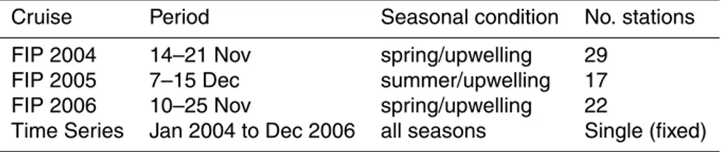
Cruise Period Seasonal condition No. stations

FIP 2004 14–21 Nov spring/upwelling 29

FIP 2005 7–15 Dec summer/upwelling 17

FIP 2006 10–25 Nov spring/upwelling 22

(22)

BGD

12, 3057–3099, 2015

R. Escribano et al.

Title Page

Tables Figures

◭ ◮

Back Close

Full Screen / Esc

Discussion

P

a

per

|

Discussion

P

a

per

|

Discussion

P

a

per

|

Discussion

P

a

per

|

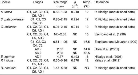
Table 2.C-specific growth rates and size ranges for different developmental stages of cope-pods from the coastal upwelling zone offChile. Estimated growth rates (g) were obtained from the molting rate method applied under in situ simulated conditions. Developmental stages are copepodids (C1 to C5) and adult females (AD♀₎)

Specie Stages Size range g Temp. Reference (mm) (d−1) (◦C)

A. tonsa C1, C2, C3, C4, 0.53–1.33 0.248 12 P. Hidalgo (unpublished data) C5, AD♀)

C. patagoniensis C1, C2, C3 0.85–2.15 0.294 12 P. Hidalgo (unpublished data) C4, C5.

C. chilensis C1, C2, C3, C4, 0.94–2.45 0.214 12 P. Hidalgo (unpublished data) C5, AD♀)

C1, C2, C3, C4, ND–2.33 ND 15 Escribano et al. (1998) C5, AD♀)

C1, C2, C3 0.61–1.96 ND 16.5 Escribano and McLaren (1999) C4, C5.

AD♀) _2.55 _ND _14.6 _{Ulloa et al. (2001)} AD♀) _2.35 _ND _18.5

E. inermis AD♀) _4.77 _0.193 ₁₆ _{Hidalgo et al. (2005)}

P. indicus C1, C2, C3, C4, 0.35–0.96 0.270 12 Yáñez et al. (2012) C5, AD♀)

(23)

BGD

12, 3057–3099, 2015

R. Escribano et al.

Title Page

Tables Figures

◭ ◮

Back Close

Full Screen / Esc

Discussion

P

a

per

|

Discussion

P

a

per

|

Discussion

P

a

per

|

Discussion

P

a

per

Table 3.Estimated copepod abundance (N), copepod biomass (CB) and copepod production (CB) from the coastal upwelling zone of Central/southern Chile, based on spatial cruises (FIP) and a time series study at Station 18. Mean±SD are shown.nrepresent the number of stations for each FIP cruise and the number of samples months for each year, respectively.

Spatial surveys Times series

Year N(Ind m−3) CB (mg C m−2) CP (mg C m−2d−1) n N(Ind m−3) CB (mg C m−2) CP (mg C m−2d−1) n

2004 50±76 449±65 12±17 22 435±337 711±577 164±128 9

2005 219±262 773±1412 193±351 17 199±306 281±451 65±99 10 2006 364±778 515±1138 130±288 22 215±178 279±276 67±65 12

(24)

BGD

12, 3057–3099, 2015

R. Escribano et al.

Title Page

Tables Figures

◭ ◮

Back Close

Full Screen / Esc

Discussion

P

a

per

|

Discussion

P

a

per

|

Discussion

P

a

per

|

Discussion

P

a

per

|

Table 4.Copepod species classified by size ranges as found during the spatial cruises in the coastal upwelling zone of Central/southern Chile. Species abundance is shown as mean±SD for each year.

Abundance [Nm−3]

Size Specie 2004 2005 2006

Small Acartia tonsa – 72.2±5.90 60.0±190.07

[<1.5 mm] Corycaeusspp. – 19.0±33.36 5.3±8.85

Oithonasimilis 34.6±49.62 23.8±53.26 48.1±60.20

Oncaeaspp. – 8.6±7.93 58.5±190.62

Paracalanus CF. indicus 33.5±37.00 65.2±60.99 180.0±440.31

Medium Centropagesbrachiatus – 4.2±4.97 3.0±3.20

[1.5–2.5 mm] Pleuromammagracilis – 8.0±9.61 16.8±27.49

Large Calanoides patagoniensis – 62.2±ND 62.3±71.23

[>2.5 mm] Calanus chilensis 1.1±2.41 90.2±191.22 29.9±76.04

Eucalanusspp. – 1.2±1.29 –

Metridiaspp. – – 5.5±13.54

(25)

BGD

12, 3057–3099, 2015

R. Escribano et al.

Title Page

Tables Figures

◭ ◮

Back Close

Full Screen / Esc

Discussion

P

a

per

|

Discussion

P

a

per

|

Discussion

P

a

per

|

Discussion

P

a

per

Table 5. Results from a generalized linear model (GLM) to test the influence of oceano-graphic variability on copepod abundance (N) and copepod production (CP), estimated from spatial cruises carried out during upwelling conditions in the coastal upwelling zone off Cen-tral/southern Chile. Only significant (P <0.05) or nearly significant (0.05< P <0.10) are shown.

Dependent Source tvalue P variable variation

N Year 3.077 0.003

Chla 1.772 0.082

CP

(26)

BGD

12, 3057–3099, 2015

R. Escribano et al.

Title Page

Tables Figures

◭ ◮

Back Close

Full Screen / Esc

Discussion

P

a

per

|

Discussion

P

a

per

|

Discussion

P

a

per

|

Discussion

P

a

per

|

(27)

BGD

12, 3057–3099, 2015

R. Escribano et al.

Title Page

Tables Figures

◭ ◮

Back Close

Full Screen / Esc

Discussion

P

a

per

|

Discussion

P

a

per

|

Discussion

P

a

per

|

Discussion

P

a

per

(28)

BGD

12, 3057–3099, 2015

R. Escribano et al.

Title Page

Tables Figures

◭ ◮

Back Close

Full Screen / Esc

Discussion

P

a

per

|

Discussion

P

a

per

|

Discussion

P

a

per

|

Discussion

P

a

per

|

(29)

BGD

12, 3057–3099, 2015

R. Escribano et al.

Title Page

Tables Figures

◭ ◮

Back Close

Full Screen / Esc

Discussion

P

a

per

|

Discussion

P

a

per

|

Discussion

P

a

per

|

Discussion

P

a

per

(30)

BGD

12, 3057–3099, 2015

R. Escribano et al.

Title Page

Tables Figures

◭ ◮

Back Close

Full Screen / Esc

Discussion

P

a

per

|

Discussion

P

a

per

|

Discussion

P

a

per

|

Discussion

P

a

per

(31)

BGD

12, 3057–3099, 2015

R. Escribano et al.

Title Page

Tables Figures

◭ ◮

Back Close

Full Screen / Esc

Discussion

P

a

per

|

Discussion

P

a

per

|

Discussion

P

a

per

|

Discussion

P

a

per

Figure 5.Time series of temperature(a), salinity(b), dissolved oxygen(c)and chlorophyll a

(32)

BGD

12, 3057–3099, 2015

R. Escribano et al.

Title Page

Tables Figures

◭ ◮

Back Close

Full Screen / Esc

Discussion

P

a

per

|

Discussion

P

a

per

|

Discussion

P

a

per

|

Discussion

P

a

per

(33)

BGD

12, 3057–3099, 2015

R. Escribano et al.

Title Page

Tables Figures

◭ ◮

Back Close

Full Screen / Esc

Discussion

P

a

per

|

Discussion

P

a

per

|

Discussion

P

a

per

|

Discussion

P

a

per

(34)

BGD

12, 3057–3099, 2015

R. Escribano et al.

Title Page

Tables Figures

◭ ◮

Back Close

Full Screen / Esc

Discussion

P

a

per

|

Discussion

P

a

per

|

Discussion

P

a

per

|

Discussion

P

a

per

|

(35)

BGD

12, 3057–3099, 2015

R. Escribano et al.

Title Page

Tables Figures

◭ ◮

Back Close

Full Screen / Esc

Discussion

P

a

per

|

Discussion

P

a

per

|

Discussion

P

a

per

|

Discussion

P

a

(36)

BGD

12, 3057–3099, 2015

R. Escribano et al.

Title Page

Tables Figures

◭ ◮

Back Close

Full Screen / Esc

Discussion

P

a

per

|

Discussion

P

a

per

|

Discussion

P

a

per

|

Discussion

P

a

per

|

(37)

BGD

12, 3057–3099, 2015

R. Escribano et al.

Title Page

Tables Figures

◭ ◮

Back Close

Full Screen / Esc

Discussion

P

a

per

|

Discussion

P

a

per

|

Discussion

P

a

per

|

Discussion

P

a

(38)

BGD

12, 3057–3099, 2015

R. Escribano et al.

Title Page

Tables Figures

◭ ◮

Back Close

Full Screen / Esc

Discussion

P

a

per

|

Discussion

P

a

per

|

Discussion

P

a

per

|

Discussion

P

a

per

|

(39)

BGD

12, 3057–3099, 2015

R. Escribano et al.

Title Page

Tables Figures

◭ ◮

Back Close

Full Screen / Esc

Discussion

P

a

per

|

Discussion

P

a

per

|

Discussion

P

a

per

|

Discussion

P

a

(40)

BGD

12, 3057–3099, 2015

R. Escribano et al.

Title Page

Tables Figures

◭ ◮

Back Close

Full Screen / Esc

Discussion

P

a

per

|

Discussion

P

a

per

|

Discussion

P

a

per

|

Discussion

P

a

per

|

(41)

BGD

12, 3057–3099, 2015

R. Escribano et al.

Title Page

Tables Figures

◭ ◮

Back Close

Full Screen / Esc

Discussion

P

a

per

|

Discussion

P

a

per

|

Discussion

P

a

per

|

Discussion

P

a

per

(42)

BGD

12, 3057–3099, 2015

R. Escribano et al.

Title Page

Tables Figures

◭ ◮

Back Close

Full Screen / Esc

Discussion

P

a

per

|

Discussion

P

a

per

|

Discussion

P

a

per

|

Discussion

P

a

per

|

(43)

BGD

12, 3057–3099, 2015

R. Escribano et al.

Title Page

Tables Figures

◭ ◮

Back Close

Full Screen / Esc

Discussion

P

a

per

|

Discussion

P

a

per

|

Discussion

P

a

per

|

Discussion

P

a

per