A Work Project, presented as part of the requirements for the Award of a Master
Degree in Finance from the NOVA – School of Business and Economics.
LIQUID INSTITUTIONS’ RESPONSE TO THE PRESENCE OF
SHORT SELLERS IN THE MARKET
JOANA CAROLINA CARVALHO OLIVEIRA, 2457
Project carried out on the Master in Finance Program, under the supervision of:
Professor Melissa Prado
Liquid institutions’ response to the presence of short sellers in the
market
ABSTRACT
The aim of this study is to examine the influence of institutions' liquidity on the level of
lending supply, short sale constraints and future stock returns, after an increase in shorting
demand. By considering the interaction between outward demand shocks and the level of
institutions’ liquidity we find that, in times of increasing shorting demand, the level of
institutions’ liquidity is not responsible for either restricting the entrance of novel short sellers
in the market or hurting existing ones; in addition, we do not find evidence of any decrease in
lending supply or future returns, nor increases in loan fees or arbitrage risk.
Keywords: Short sale constraints, liquid institutional investors, equity-lending supply, stock
I. Introduction
Classical asset-pricing models assume investors can act freely within the stock market,
buying, selling and short selling securities at no cost. Hence, when determined security is
detected as being overpriced, investors can act accordingly, selling or short selling it, in order
to reestablish its fair price. In reality, however, while buying and selling are seen as
straightforward operations, short selling can be difficult, risky and costly, due to the
characteristics of the equity lending market.
According to the U.S Securities and Exchange Commission (SEC) a short sale is “the
sale of a security that the seller does not own or that the seller owns but does not deliver. In
order to deliver the security to the purchaser the short seller will borrow the security, typically
from a broker-dealer or an institutional investor”1. The lending market is where short sellers
are matched with owners of the security able and willing to lend their shares for a fee. Since
the lending market is an over-the-counter market, when an investor considers the short sale of
an overpriced security, she has to take into account the necessity of incurring a security loan
transaction that can be both difficult to find and expensive. These risks and costs are usually
referred to as short sale constraints and are responsible for maintaining short sellers out of the
stock market, reducing market efficiency and increasing mispricing. Indeed, Diamond, and Verrecchia (1987) argue that short sellers will not trade unless the expected fall in the price of the security is enough to justify the costs and risks associated with the short selling position.
Miller (1977) argues that short sale constraints keep pessimistic investors out of the market, causing overpricing.
With this study we aim to complement prior literature, which has explored the sources
of short sale constraints. Although many studies have argued that the level of short sale
constraints can be measured by lending supply (for example, Saffi and Sigurdsson (2011)),
proxied by the level of institutional ownership (D’Avolio (2002), Chen, Hong, and Stein (2002), Nagel (2005)), Prado, Saffi and Sturgess (2014) show that total institutional ownership is not a sufficient proxy for lending supply constraints, being necessary to take its
composition into consideration. Our goal is to assess the influence of institutional ownership
composition by studying how liquid institutions (deep pocket institutions) react to the
presence of short sellers in the stock market. The following example illustrates the importance
of studying this relationship. In the beginning of 2012, Herbalife’s level of short interest
started to increase. Among other investors, Bill Ackman, the head of Pershing Square Capital
Management, believed that Herbalife was running a pyramid scheme and, therefore, that its
price was going to decrease to zero in the future. In December of 2012 Ackman’s hedge fund
revealed an uncovered short position of $1 billion in HLF’s stock (approximately 20% of
HLF’s float). One would expect the price of the stock to decrease with this shorting activity,
however, in the beginning of 2013 some big and liquid funds, and some wealthy individuals,
like George Soros, started to buy Herbalife’s stock. Due to the high quantity of shares held on
the short side, when the big funds entered the market buying Herbalife shares, squeezing the
price higher, Ackman’s fund started to struggle. The size of the struggle was even bigger if
we were to consider the large amount the fund had to spend per year to maintain the short
position. According to “The Fortune”, Herbalife’s stock would have to be trading at the low
30s in order for Pershing Square to break even on its position (without considering the margin
costs). At the 21st of June of 2016, the stock was trading at $59.38.
We hypothesize that liquid investors have a specific behavior within the market, when
facing an increase in the level of shorting demand. Their high level of liquidity provides them
the capacity of influencing both the equity lending market and the stock market. Hence, we
posit that, according to the preferences of the shareholders, these institutions are able to
short sale constraints will be observed, not followed by an increase in the level of negative
future returns, resulting in a decrease in the net returns of short positions. They are, therefore,
able to deliberately squeeze short sellers out of their short positions.
In order to perform our analysis we use equity-lending data from Markit, ownership
data from Thomson-Reuters Institutional Holdings (13F), and pricing and accounting data
from CRSP and Compustat.
For each of the 5,277 U.S stocks present in the sample, we use the holdings provided
in the institutional ownership dataset to compute a measure of illiquidity. We use this as a
proxy for the level of liquidity each institutional investor achieves by holding the stock. Then,
we combine this measure with the methodology developed by Cohen, Diether, and Malloy (2007) in order to examine how institutions react to an increasing presence of short sellers in the market. With the objective of better understanding the effects of institutional ownership
structure on the equity lending market and stock market, we examine the consequences of
having liquid institutions, in times of increasing shorting demand, for the level of equity
lending supply, short sale constraints and future returns.
We find that, following an outward demand shift the level of investors’ liquidity does
not affect the level of lending supply. Deep pocket investors are, therefore, not able to limit
short sellers’ ability to take short positions by conditioning the level of shares available to be
borrowed. The evidence for the level of short sale constraints goes against our premises. We
hypothesize that, in the presence of an increasing shorting demand, higher institutions’
liquidity should be associated with higher short sale constraints, measured by higher
borrowing fees and higher idiosyncratic volatility of returns. In the following quarter,
abnormal returns would not be more negative and, thus, a decrease in the net returns of short
positions would be observed. After examining the data, we find no indication of an existing
Additionally, we find evidence that a higher presence of deep pocket institutions in the market
leads to a decrease in the borrowing fee. All our estimations include firm fixed-effects,
year-quarter dummies and double-clustered standard errors at stock and year-quarterly levels.
The remainder of the study proceeds as follows. Section II reviews the existing
literature on the effects of ownership structure on lending and stock markets. Section III
describes the data and discusses methodology. Section IV contains the empirical results.
Section V concludes.
II. Literature Review
Once a short position is initiated, the short seller has to find an investor willing to lend
the desired stock. Since often not all the shares outstanding are available to be borrowed, the
supply of lendable shares will affect the size of the short positions that can be taken at low
cost (low borrowing fee). Therefore, investors’ disposition to lend shares will influence the
costs that short sellers have to bear when borrowing the stock. Indeed, Beneish, Lee, and Nichols (2013) find that stocks that are difficult to borrow have less than 10 percent of easily lendable shares out of their outstanding shares. Further, for easy-to-borrow stocks the average
number of easily lendable shares is typically only 20 percent of shares outstanding. D’Avolio (2002) finds that the main suppliers of stock loans are institutional investors. Additionally, the author finds that stocks with low institutional ownership are more expensive to borrow. Chen, Hong, and Stein (2002) argue that breadth of ownership, quantified by the percentage of institutions owning the stock, is a measure of the ease with which shares can be borrowed.
Kolasinski, Reed, and Ringgenberg (2013) model the loan supply curve and find a U-shaped relation between institutional ownership and loan fees. This relation is more steeply upward
sloping when stocks are smaller, less liquid and have loan volume dispersed among many
lenders.
not sufficient to study lending supply constraints. These authors find that, additionally to the
level of total institutional ownership, its composition is important to explain the amount of
lending supply and short sale constraints present in the lending market. Some prior studies
share this idea. As holders of a large amount of stocks, institutional investors are able to
decide if they want to participate in the equity lending market and in which scale. Evans, Ferreira, and Prado (2012) show that different types of institutional investors have different preferences about the size of the equity-lending program to implement. For example, while it
is very likely that index funds engage in a large lending program, actively managed funds
have to decide whether this decision is valuable; although equity-lending programs have the
capacity to generate additional returns to the funds, Chuprini, and Massa (2012) show that the decision to make shares available for borrowing is taken considering stocks’ characteristics
within the managers’ portfolio. Aggarwal, Saffi, and Sturgess (2013) show that many institutional investors are interested in holding voting rights at the time of shareholder
meetings. For this reason, it is expected the recall of many equity loans around these meeting
dates.
Short selling is a trading strategy designed to correct overpricing. In prior literature,
short sellers are accepted as sophisticated investors (for example, Drake, Rees, and Swanson (2002) and Dechow et al. (2001)) that help to incorporate information into the financial markets, increasing efficiency. Boehmer, and Wu (2013) focus on short sellers’ daily trading activity and find that they are able to improve the information efficiency of prices. Hence, if
short sale constraints retain short sellers out of the market, limits to arbitrage will arise. This
relationship between the equity lending market and the stock market has been extensively
studied. Some earlier papers used the short interest ratio (SIR) as a proxy for short selling
demand in order to study the level of mispricing existent in the stock market. However, it has
excluded from the stock market: the short interest ratio can be low either because demand is
low, or because supply is limited. Hence, more recent studies have been aiming to incorporate
supply in their analysis. For example, Nagel (2005) and Hirshleifer, Teoh, and Yu (2011) use the percentage of institutional holdings as a proxy for the level of supply and suggest that
negative future returns are related to the existence of short selling constraints, being more
negative when institutional ownership is low (short selling constraints are high). Autore, Boulton, and Braga Alves (2010) argue one should analyze stock prices when short sale constraints are tightening. To perform the analysis the authors use threshold events and argue
that threshold stocks are short sale constrained, becoming overpriced. The extent of the
overpricing is directly related to the level of failures to deliver, which indicate how tightly
short sale constraints are. Drechsler, and Drechsler (2014) argue that the average returns short sellers receive significantly exceed the fees they pay. For the authors, this shorting
premium reflects compensation for bearing the risk involved in shorting high-fee stocks.
Differently, Cohen, Diether, and Malloy (2007) create a methodology to distinguish supply from demand shocks and believe that shorting demand is a significant predictor of future
stock returns while supply plays a minor role. Kaplan, Moskowitz, and Sensoy (2013)
consider that equity lending supply does not influence stock prices.
Institutional investors have, in general, a greater ability and predisposition to lend
shares to be shorted. However, there are some institutions that, due to their characteristics,
have high bargaining power and are not willing to lend shares as the general ones. The
necessity of having a stock market efficient can, therefore, be overcame by the preferences of
these institutions. Our study desires to show that if managers of deep pocket institutions
prefer to maintain high valuations to show performance, these managers will try to limit the
III. Methodology
A. Hypotheses
To study the behavior and influence of deep pocket institutions in the lending and
stock markets we test four hypotheses.
Although prior literature has argued that the level of institutional ownership explains
an important portion of lending supply, Prado, Saffi and Sturgess (2014) show that the composition of institutional ownership also has a role in this play. For the authors, highly
concentrated institutional ownership results in shareholders having considerable influence in
the equity lending market. We consider that institutional ownership composition, measured by
the level of deep pocket institutions present in the market, also has an important impact in
both the lending and stock market.
Highly liquid institutions are able to exercise some pressure in prices, according to
their preferences. We anticipate that, in times of increasing shorting demand, deep pocket
institutions will hold onto their holdings, or even increase them, leading to the limiting of the
lending supply level. With this, institutions are able to keep short sellers from decreasing
stock prices.
Hypothesis 1: Although there is an increase in demand for shorting, a decrease in lending supply is expected when the level of institutions’ liquidity increases.
In order to borrow a stock, the short seller must place collateral. If the collateral is
cash, the loan fee is defined as the difference between the risk-free interest rate and the rebate
rate. The rebate rate is the remuneration the lender gives to the borrower on the collateral left
with the lender. When the collateral is not cash, borrowers and lenders directly negotiate the
the availability of the stock for borrowing, and the risk that the short position is involuntarily
closed due to recall of the stock loan. Additionally, Shleifer and Vishny (1997) argue that idiosyncratic volatility can also be considered an important risk for short positions. Since this
type of volatility cannot be hedged, when entering in high idiosyncratic volatility positions
short sellers are engaging in a higher risk of having to close positions before the desired time.
These costs and risks are known as short sale constraints and are responsible for transforming
short selling in an expensive and risky trading strategy. Our objective is to understand how
the institutions’ level of liquidity can influence these constraints, in times of increasing
shorting demand. To do that we consider two measures: borrowing fee and idiosyncratic
volatility of returns. The first reflects the direct cost of taking a short position, and the second
measures the level of arbitrage risk and reflects the risk of having a short position being
closed before desired due to short-term losses that cannot be hedged.
Hypothesis 2: Deep pocket risk - the ability to squeeze short sellers out of the market - should positively impact short sale constraints, measured by borrowing fees, when an increase in demand for shorting is observed.
Hypothesis 3: Deep pocket risk - the ability to squeeze short sellers out of the market - should positively impact short sale constraints, measured by arbitrage risk, when an increase in demand for shorting is observed.
If higher investors’ liquidity results in higher short sale constraints and increases
arbitrage risk, one would be willing to accept that future returns will be more negative,
increasing short sellers’ gross returns. However, it is our conviction that when deep pocket
institutions are interested in maintaining high valuations, they will find ways to influence the
market, not allowing short sellers’ returns to increase.
to limit the incorporation of negative information by squeezing investors out of the market.
According to our scenario short sellers will have less opportunities to enter the market
and, thus, to correct overpricing since borrowing costs increase at the same time that future
returns remain the same or decrease.
B. Data
We use equity lending data, ownership data, pricing data and accounting data,
obtained from four different sources, between August 1st, 2006 and December 31st, 2010 to
test all the proposed hypotheses.
From Thomson-Reuters Institutional Holdings (13F) database we obtain institutional
common stock holdings, as reported on Form 13F filed with the SEC. This form is filed on a
quarterly basis and contains ownership information provided by institutional managers with
100 million dollars or more in assets under management. The equity lending data is obtained
from Markit. Markit collects this type of security-level daily information from more than 125
custodians and 32 prime brokers. Pricing data and accounting data are obtained from CRSP
and Compustat, respectively.
We match the firms available on the equity-lending database with the ones present in
CRSP. After the matching we have 5,277 U.S stocks to work with. Additionally, and since the
ownership data is only reported at a quarterly frequency, we compute quarterly averages of
daily pricing and lending variables for each firm. To ensure that microcap stocks or low share
price observations do not explain the majority our results, we do not consider any observation
for which the stock price is below or equal to $1. Additionally, to reduce the impact of
outliers in our results, all the variables are winsorized at 1%-level. In order to guarantee that
all the stocks that we are considering for our analysis have lending and return data available,
C. Methodology
Using ownership data from Thomson Reuters we calculate, for each of the 5,277
stocks in our sample, the ownership by each institution, total institutional ownership,
concentration of institutional holdings and the fraction held by passive investors, as in Prado, Saffi and Sturgess (2014). We also compute ∆Breadth as in Chen, Hong, and Stein (2002). From CRSP and Compustat data we compute market capitalization, cumulative quarterly
returns, standard deviation of daily returns, turnover, book-to-market ratio, cumulative
abnormal returns based on Daniel et al. (1997) characteristics-matched factor, and idiosyncratic risk as being the mean squared error of residuals from Cahart (1997)’s 4-factor model.
We additionally compute our measure of investors’ liquidity: DPocket. Since liquidity
represents the ability to convert stocks into cash (or vice versa), we compute the Amihud
Illiquidity across institutions’ holdings and take a weighted average (using the portfolio size
as weight) at the institution level. We argue that this can measure the difficulty with which
institutions can trade the stock and, hence, the level of liquidity (deep pockets) institutions
can achieve by holding each stock. The higher is the value of our variable, the higher is the
Amihud Illiquidity and the less liquid institutions can be.
The methodology developed by Cohen, Diether, and Malloy (2007) is used to test all the hypotheses. Cohen, Diether, and Malloy (2007) argue that we are able to distinguish demand from supply shifts using price-quantity “pairs” from the equity lending market. For
these authors, when there is both an increase in the loan fee (price) and in the percentage of
shares on loan (quantity), the lending market experienced at least an outward demand shift
(i.e, there was at least an increase in shorting demand - DOUT). Following the same
reasoning, an inward shift in shorting demand (i.e, DIN) is observed when both the loan fee
approach2 and define:
where i and t are the stock and period in analysis, respectively. Loan is the percentage of shares on loan. Fee Score is an additional measure of loan fees computed by Markit with the
objective of measuring levels of fee that are truly different from each other. This variable can
assume values between 1 and 10 (from cheapest to hardest to borrow).
Cohen, Diether, and Malloy (2007) and Prado, Saffi and Sturgess (2014) used DOUT to prove that the level of negative abnormal returns in the following month/week could be
predicted. We propose to go beyond and use DOUT combined with institutions’ liquidity
level to analyze not only their effect on returns’ predictability but also on lending supply and
short sale constraints levels.
D. Descriptive statistics
Table I presents descriptive statistics for the most important variables used throughout
this study. As reported by Prado, Saffi and Sturgess (2014), the average firm has 20.2% of its shares outstanding available for lending; 4.8% are actually lent out, which indicates an
average utilization level (ie., amount lent out divided by the amount available to lend) of 19%.
On average, 13% of the firm-quarter observations present in our sample have borrowing fees
greater than 100 basis points and, hence, are considered to be “on special”. The average
institutional ownership is 59.2% and the average Amihud illiquidity of the holdings (our
DPocket) is 2.146.
2
1 if Fee Scoret-1 – Fee Scoret-2 >0 and Loant-1 – Loant-2>0
0 otherwise
1 if Fee Scoret-1 – Fee Scoret-2 <0 and Loant-1 – Loant-2<0
0 otherwise DOUTi,t-1 =
Table I - Descriptive Statistics
The table presents the descriptive statistics for the main variables in our study, during the sample period (August 1st, 2006 and December 31st, 2010). Equity lending data is obtained from Markit. Ownership data is obtained from Thomson-Reuters Institutional Holdings (13F), Pricing and Accounting data are obtained from CRSP and Compustat. Obs is the number of firm-quarter observations.
Variable Obs Mean Median Stdev Min Max Skewness Kurtosis
Equity lending
Lending Supply 58819 0.202 0.204 0.128 0 0.537 0.29 2.42
On loan 58819 0.048 0.026 0.058 0 0.278 1.85 6.40
Borrowing fee (bps) 58819 66.552 13.252 177.992 -6.828 1301.181 4.71 28.00
Fee score 58334 1.469 1.000 1.183 1 10 3.70 18.66
Specialness 58819 0.130 0 0.336 0 1 2.20 5.84
Utilization level (%) 58819 19.305 11.981 20.393 0 84.605 1.33 4.08
Institutional Ownership
Inst. Ownership 58819 0.592 0.648 0.300 0.0 1.000 -0.37 1.90
Dpocket 58819 2.146 0.008 11.133 0.0 112.148 7.82 69.81
Inst. Own. Concentration 58819 0.116 0.064 0.134 0.013 1.000 3.00 14.26
Portion of total shares held
by top5 inst. 58819 0.275 0.271 0.136 0.000 1.000 0.74 5.29
Top5 holdings 58819 0.538 0.470 0.220 0.153 1.000 0.68 2.28
Breadth 58819 143.75 92.00 181.36 1.00 1683.00 3.35 18.39
∆Breadth 58819 0.010 0.000 0.031 -0.043 0.186 1.40 3.63
Passive Own. 58819 0.054 0.030 0.062 0.000 0.262 1.35 4.37
Pricing and Accounting
Price 58819 24.080 15.850 67.184 1 4736.000 41.60 2277.59
Dp<5 58819 0.176 0 0.381 0 1 1.70 3.91
Market Capitalization 58819 3789.4 426.0 16541.1 1.3 513362.0 12.23 217.37
Return (quarterly) 58819 0.032 0.010 0.336 -0.878 18.332 9.17 292.84
Return (quarterly) 58819 0.034 0.028 0.025 0.001 2.448 18.41 1518.89
Arbitrage Risk 58819 0.028 0.023 0.023 0.001 2.309 19.92 1647.20
Turnover 58819 0.918 0.660 1.051 0.002 33.716 5.76 94.20
BM ratio 58819 0.741 0.576 0.658 -0.069 4.426 2.62 12.55
S&P500 indicator 58819 0.015 0.000 0.120 0.0 1.000 8.08 66.33
Number of analysts 58819 1.211 1.099 0.970 0.0 3.807 0.17 1.86
IV. Empirical Results
I. Institutions’ liquidity level and equity lending supply
In this section of our study we test whether deep pocket institutions have or not
influence in the level of lending supply, whenever there is an increase in shorting demand.
We apply multivariate regression analysis by using pooled OLS regressions with quarterly
$5 and SP500 equal to 1 if the stock belongs to the S&P500 in the present quarter. By using this set of control variables we are able to control for a number of factors such as investors’
sentiment, stock’s visibility, liquidity, size and momentum.
Column 1 of Table II summarizes the results from our analysis. We start by observing
that the coefficient for total ownership (Total) is positive and statistically significant. Hence, similarly to what previous research such as D’Avolio (2002) or Nagel (2005) has reported, we find that an increase in the amount of institutional holdings of determined stock is related to
an increase in the level of lending supply. By looking at the coefficients for outward demand
shift (DOUT) and institutions’ liquidity (DPocket), separately, we examine how increases in
demand for shorting or in institutions’ liquidity influence lending supply. Even though short
sellers are more interested in borrowing the stock (DOUT=1), we find no evidence of a
change in the level of available shares to borrow. The coefficient for institutions’ liquidity
(DPocket) is negative and statistically significant at 5%. Keeping in mind that DPocket is the
Amihud Illiquidity of the holdings of all institutions, we find evidence that an increase in the
level of institutions’ liquidity is associated with an increase in the level of shares available for
borrowing. However, our key interest when performing this regression is to test whether an
increase in demand for shorting among shares held by liquid institutions influences lending
supply. We find that the coefficient for the interaction between DOUT and DPocket is not
statistically significant and, therefore, we find no evidence supporting our first hypothesis. A
conceivable explanation for this result is the possibility that the relationship between
institutions’ liquidity and lending supply only exists when stocks are predominantly held by
institutional investors. To study this new hypothesis, we create an indicator variable (BigIO) equal to 1 if the stock belongs to the top quartile of institutional ownership. The second
relationship between lending supply and deep pocket institutions with significantly high
holdings.
Table II - Investors' liquidity on Lending Supply
The table displays OLS regressions of equity lending supply as a function of ownership composition measures. We use quarterly U.S stock data between August 2006 and December 2010. Equity lending data is obtained from Markit. Ownership data is obtained from Thomson-Reuters Institutional Holdings (13F), Pricing and Accounting data are obtained from CRSP and Compustat. All variables are standardized to have mean zero and standard deviation equal to one. The regression includes stock fixed-effects and year-quarter dummies. Standard errors are double-clustered at the firm and quarter levels. Standard errors are reported in brackets and significance levels are reported as follows: *** p<0.01, ** p<0.05, * p<0.1
Lending Supply
1 2
Total 0.453*** 0.460***
[0.027] [0.025]
DOUTt -0.014 -0.009
[0.011] [0.011]
Dpocket -0.005** -0.004**
[0.002] [0.002]
Dpocket*DOUTt -0.003 -0.004
[0.007] [0.007]
Dpocket*BigIO 0.060
[0.082]
Dpocket*BigIO*DOUTt 0.167
[0.130]
∆Breadth -0.007 -0.007
[0.009] [0.009]
MarketCap. 0.479*** 0.478***
[0.063] [0.062]
Dp<5 -0.047* -0.048*
[0.026] [0.025]
Turnover 0.025*** 0.025***
[0.008] [0.008]
BM 0.219*** 0.219***
[0.019] [0.019]
Momentum -0.002 -0.002
[0.005] [0.005]
Sp500 -0.099 -0.099
[0.312] [0.312]
Number_analysts 0.015*** 0.015***
[0.004] [0.004]
Observations 54,887 54,887
Number of isinn 4,288 4,288
R-squared 0.192 0.192
Adjusted R-squared 0.123 0.123
While interpreting this result, one should take into account the indirect method we are
currently using to measure deep pocket risk. It is our belief that by using a more direct
deep pocket institutions and the level of lending supply, after any outward demand shock.
II. Institutions’ liquidity level and short sale constraints
We measure the level of short sale constraints by focusing on borrowing costs and
arbitrage risk. Loan fees, the direct costs of borrowing, are considered the most direct form of
short sale constraints since they reflect the fee short sellers have to pay in order to borrow the
stock they desire to short. Arbitrage risk represents the fragment of returns that cannot be
explained by standard risk factors and, therefore, is a measure of the risk that short sellers
have to take when correcting overpricing. We measure arbitrage risk as being the mean
squared error of daily stock returns’ residuals from the 4-factor model present by Cahart (1997). Since investors have limited capital and always desire to maximize their net returns, an increase in the level of loan fees or arbitrage risk will decrease the opportunities for an
investor to take on a short position. We apply multivariate regression analysis by using pooled
OLS regressions with quarterly data. The set of control variables is as presented in Table II.
Using Panel a) in Table III we can see that an increase in the level of demand for
shorting is associated with a 53 bps increase in the price of the loan. However, our primary
aim is to show that more liquid institutions are able to both influence the level of lending
supply and contribute to an increase in the loan costs, when an outward demand shift is
observed. We find no evidence supporting our assumption. Table III presents the coefficient
for the interaction between DOUT and DPocket; it is statistically significant at 10% and
indicates that, after an outward demand shock, the presence of more liquid institutions in the
market is associated with a decrease of 12.0% (!.!"#∗!"".!!"
!!.!!" ) in the average level of fees that
short sellers have to pay to borrow the stocks. Our findings do not change if we include the
concentration and composition measures used by Prado, Saffi and Sturgess (2014) as control variables: a unit standard deviation increase in investors’ liquidity is associated with loan fees
being 0.046 standard deviations lower, equivalent to a 12.3% (!.!"#∗!"".!!"
to the average borrowing fee.
Table III - Investors' liquidity on short sale constraints
The table displays OLS regressions of a) borrowing costs and b) arbitrage risk as a function of ownership composition measures. Borrowing costs are measured by loan fees. Arbitrage risk is measured as the standard deviation of daily stock returns’ residuals from Cahart (1997)'s 4-factor model. We use quarterly U.S stock data between August 2006 and December 2010. Equity lending data is obtained from Markit. Ownership data is obtained from Thomson-Reuters Institutional Holdings (13F), Pricing and Accounting data are obtained from CRSP and Compustat. All variables are standardized to have mean zero and standard deviation equal to one. The regressions include stock fixed-effects and year-quarter dummies. Standard errors are double-clustered at the firm and quarter levels. Standard errors are reported in brackets and significance levels are reported as follows: *** p<0.01, ** p<0.05, * p<0.1
a) Borrowing costs b) Arbitrage risk
1 2 3 4 1 2 3 4
Total -0.054** -0.044 -0.030 -0.030 -0.118*** -0.111*** -0.106*** -0.107***
[0.027] [0.027] [0.027] [0.027] [0.018] [0.018] [0.017] [0.017]
DOUTt 0.532*** 0.531*** 0.530*** 0.530*** 0.117*** 0.117*** 0.116*** 0.117***
[0.060] [0.060] [0.060] [0.060] [0.027] [0.028] [0.028] [0.028]
Dpocket -0.002 -0.004 -0.003 -0.003 0.075*** 0.074*** 0.075*** 0.074***
[0.009] [0.009] [0.009] [0.009] [0.014] [0.014] [0.014] [0.014]
Dpocket* DOUTt
0.045* 0.046* 0.047* 0.046* -0.005 -0.005 -0.005 -0.005 [0.024] [0.024] [0.024] [0.024] [0.028] [0.027] [0.028] [0.027]
Top5 0.094*** 0.069*** 0.040*** 0.020
[0.021] [0.023] [0.013] [0.025]
HHI 0.069*** 0.042* 0.041 0.033
[0.022] [0.024] [0.026] [0.034]
% Passive 0.002 0.001 0.001 -0.008* -0.008* -0.008*
[0.004] [0.004] [0.004] [0.004] [0.004] [0.004]
∆Breadth 0.000 -0.002 -0.003 -0.003 -0.018 -0.019* -0.019* -0.020*
[0.011] [0.010] [0.011] [0.010] [0.011] [0.011] [0.011] [0.011]
MarketCap. -0.409*** -0.387*** -0.358*** -0.358*** -0.823*** -0.808*** -0.799*** -0.800***
[0.055] [0.056] [0.055] [0.055] [0.049] [0.053] [0.052] [0.052]
Dp<5 -0.075*** -0.078*** -0.077*** -0.078*** 0.237*** 0.235*** 0.236*** 0.235***
[0.025] [0.025] [0.025] [0.025] [0.032] [0.033] [0.032] [0.033]
Turnover 0.083*** 0.086*** 0.090*** 0.089*** 0.412*** 0.413*** 0.415*** 0.414***
[0.014] [0.014] [0.014] [0.014] [0.021] [0.021] [0.021] [0.021]
BM 0.016 0.016 0.016 0.016 -0.025** -0.024* -0.024** -0.024*
[0.015] [0.015] [0.015] [0.015] [0.012] [0.012] [0.012] [0.012]
Momentum 0.010* 0.010* 0.010* 0.010* -0.002 -0.002 -0.002 -0.002
[0.006] [0.006] [0.006] [0.006] [0.009] [0.009] [0.009] [0.009]
Sp500 0.136** 0.127* 0.103 0.107 0.117 0.112 0.103 0.106
[0.068] [0.071] [0.089] [0.085] [0.157] [0.153] [0.144] [0.148]
Number analysts
0.012** 0.012** 0.013** 0.013** -0.012** -0.012** -0.012** -0.012** [0.006] [0.006] [0.006] [0.006] [0.006] [0.006] [0.006] [0.006]
Observations 54,887 54,887 54,887 54,887 54,887 54,887 54,887 54,887
Number of
isinn 0.055 0.056 0.056 0.057 0.242 0.242 0.242 0.243
R-squared 4,288 4,288 4,288 4,288 4,288 4,288 4,288 4,288
Adj.
R-squared -0.0262 -0.0247 -0.0244 -0.0240 0.177 0.178 0.178 0.178
Panel b) in Table III describes the influence of outward demand shifts and investors’
DOUT and DPocket are statistically significant, the coefficient for their interaction is not.
Once more, the evidence present in the data deviates from our predictions; in times of
increasing shorting demand, the level of investors’ liquidity does not influence the arbitrage
risk short sellers have to face when holding a short position.
III. Institutions’ liquidity level and future stock returns
In hypothesis 4 we state that, after an increase in shorting demand, abnormal returns in
the following quarter will not be more negative for stocks being held by the most liquid
institutions.
As in Prado, Saffi and Sturgess (2014), firstly we analyze this hypothesis with a portfolio-analysis approach. We distribute all the stocks across two demand shift portfolios:
DOUT=1 and DOUT=0, where DOUT is equal to 1 if the stock has experienced an outward
demand shift last quarter. Then, we split the stocks that belong to each of these two portfolios
into two additional portfolios: Top(DPocket)=1 and Top(DPocket)=0, where Top(DPocket) is equal to 1 if the stock was in the bottom quartile of the Amihud Illiquidity measure, last
quarter. Stocks in this situation are considered to be the stocks with which institutions can
achieve the highest level of liquidity. The stocks are considered to be in the portfolios during
quarter t, existing a rebalancing every quarter. For each of the four portfolios we compute
abnormal returns. The abnormal returns are calculated as the difference between the quarterly
stock return and the return based on a characteristics-matched benchmark portfolio sorted on
market capitalization, B/M ration and momentum, as in Daniel et al. (1997). Our results are presented in Table IV. We find evidence that, when no outward demand shift occurs, stocks
being held by the most liquid institutions have abnormal returns 0.009% lower in the
following quarter, when compared to those that are not held by liquid investors. However,
there is no evidence that returns can be predicted, when an outward demand shift occurs. The
Table IV – Abnormal Returns sorted on DOUT and DPocket portfolios
Table IV presents U.S stocks abnormal returns of portfolios sorted first on outward demand shifts (DOUT) in the previous quarter and, then, on investors' liquidity levels, during the sample period (August 1st, 2006 and December 31st, 2010). Equity lending data is obtained from Markit. Ownership data is obtained from Thomson-Reuters Institutional Holdings (13F). DOUT is an indicator variable equal to 1 if, in the previous quarter, an outward demand shift was observed. Top(DPocket) is an indicator variable equal to 1 if, last quarter, the stock was in the bottom quartile of the Amihud illiquidity measure, conditionally on DOUT. Equity lending data is obtained from Markit. Ownership data is obtained from Thomson Reuters. Significance levels are reported as follows: *** p<0.01, ** p<0.05, * p<0.1
Additionally, we present the effect of deep pocket institutions on future abnormal
returns, when there is an outward demand shift, using a multivariate regression analysis. We
estimate pooled OLS regressions with quarterly data using a wide array of control variables,
as in Prado, Saffi and Sturgess (2014). Bottom(Supply), Top(RMSE), Top(DPocket) and
Bottom(Total) are indicator variables, calculated in the previous quarter. Bottom(Supply)
equals 1 if the firm belonged to the five percent of firms with the lowest level of lending
supply, in the previous quarter. Top(RMSE) is equal to 1 if the firm was in the top quartile of idiosyncratic risk, in the previous quarter. Bottom(Total) equals 1 if the stock was in the bottom quartile of institutional ownership, last quarter. Abret are quarterly abnormal returns, lagged one quarter.
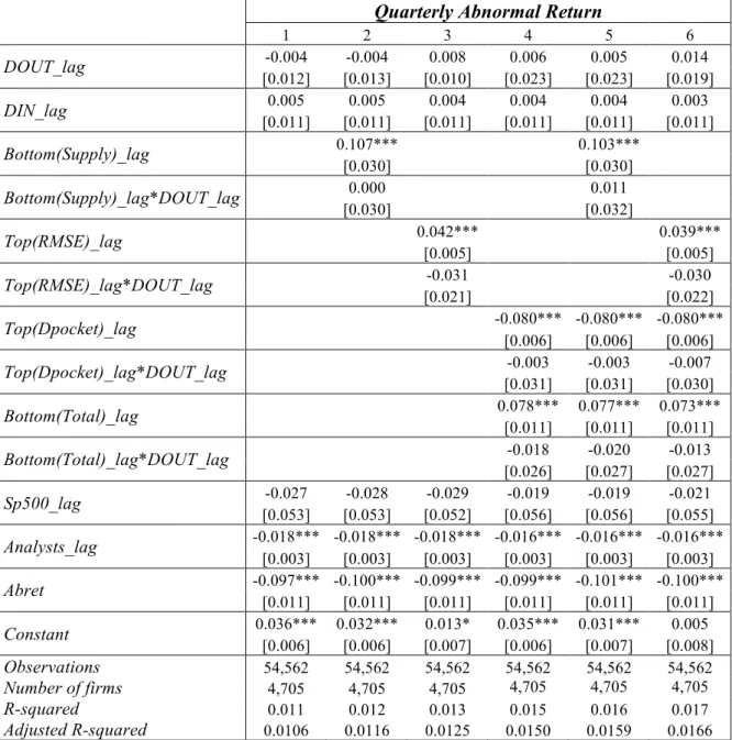
Table V depicts the results. By analyzing each column separately we find that,
although Bottom(Supply), Bottom(Total), Top(RMSE) and Top(DPocket) are able to explain
the level of abnormal returns in the following quarter, their explanatory power disappears
when we consider the existence of an outward demand shift. We believe that these results
derive from the frequency of the data used. Cohen, Diether, and Malloy (2007) found that DOUT significantly explains the level of returns in the following month and Prado, Saffi and Sturgess (2014) showed that it also explains returns in the following week. Our results seem to indicate that a quarterly frequency is not adequate to study the relation between outward
demand shifts and future returns.
DOUT \ Top(Dpocket) 0 1 1-0
0 0.0107 0.0018 -0.0089***
1 -0.0048 -0.0184 -0.0136
Table V - Investors' liquidity and demand shifts on future abnormal returns
Table V displays OLS regressions of quarterly abnormal returns as a function of lagged demand shifts and lagged ownership composition measures. We use quarterly U.S stock data between August 2006 and December 2010. Equity lending data is obtained from Markit. Ownership data is obtained from Thomson-Reuters Institutional Holdings (13F), Pricing and Accounting data are obtained from CRSP and Compustat. DOUT is an indicator variable equal to 1 if, in the previous quarter, an outward demand shift was observed. DIN is an indicator variable equal to 1 if, in the previous quarter, an inward demand shift was observed. Top(DPocket) is an indicator variable equal to 1 if, last quarter, the stock was in the bottom quartile of the Amihud illiquidity measure. Bottom(Supply) equals 1 if the firm belonged to the five percent of firms with the lowest level of lending supply, in the previous quarter. Top(RMSE) is equal to 1 if the firm was in the top quartile of idiosyncratic risk, in the previous quarter. Bottom(Total) equals 1 if the stock was in the bottom quartile of institutional ownership, last quarter. Abret are the quarterly abnormal returns, lagged one quarter. The regressions include year-quarter dummies. Standard errors are clustered at the firm level. Standard errors are reported in brackets and significance levels are reported as follows: *** p<0.01, ** p<0.05, * p<0.1
Quarterly Abnormal Return
1 2 3 4 5 6
DOUT_lag -0.004 -0.004 0.008 0.006 0.005 0.014
[0.012] [0.013] [0.010] [0.023] [0.023] [0.019]
DIN_lag 0.005 0.005 0.004 0.004 0.004 0.003
[0.011] [0.011] [0.011] [0.011] [0.011] [0.011]
Bottom(Supply)_lag 0.107*** 0.103***
[0.030] [0.030]
Bottom(Supply)_lag*DOUT_lag 0.000 0.011
[0.030] [0.032]
Top(RMSE)_lag 0.042*** 0.039***
[0.005] [0.005]
Top(RMSE)_lag*DOUT_lag -0.031 -0.030
[0.021] [0.022]
Top(Dpocket)_lag -0.080*** -0.080*** -0.080***
[0.006] [0.006] [0.006]
Top(Dpocket)_lag*DOUT_lag -0.003 -0.003 -0.007
[0.031] [0.031] [0.030]
Bottom(Total)_lag 0.078*** 0.077*** 0.073***
[0.011] [0.011] [0.011]
Bottom(Total)_lag*DOUT_lag -0.018 -0.020 -0.013
[0.026] [0.027] [0.027]
Sp500_lag -0.027 -0.028 -0.029 -0.019 -0.019 -0.021
[0.053] [0.053] [0.052] [0.056] [0.056] [0.055]
Analysts_lag -0.018*** -0.018*** -0.018*** -0.016*** -0.016*** -0.016***
[0.003] [0.003] [0.003] [0.003] [0.003] [0.003]
Abret -0.097*** -0.100*** -0.099*** -0.099*** -0.101*** -0.100***
[0.011] [0.011] [0.011] [0.011] [0.011] [0.011]
Constant 0.036*** 0.032*** 0.013* 0.035*** 0.031*** 0.005
[0.006] [0.006] [0.007] [0.006] [0.007] [0.008]
Observations 54,562 54,562 54,562 54,562 54,562 54,562
Number of firms 4,705 4,705 4,705 4,705 4,705 4,705
R-squared 0.011 0.012 0.013 0.015 0.016 0.017
Adjusted R-squared 0.0106 0.0116 0.0125 0.0150 0.0159 0.0166
The variables used in all the models except the last are standardized to have mean zero
and standard deviation one. To guarantee that our estimates are not biased due to the existence
we include firm fixed-effects in all, except the last, regressions. In addition, all regressions
include year-quarter dummies. Standard errors are double-clustered at the stock and quarterly
level for all the models except the latter; in this last model we only use standard errors
clustered at the stock level.
V. Conclusion
An investor will take on a short position if she believes it is possible to build a profit
from it. However, to sell short a stock, the investor has to locate the desired shares, often by
having to consult multiple lenders in the equity lending market. The problem of searching is
mostly known by being one of the causes of positive loan fees existence (Duffie, Gârleanu, and Pedersen (2002) and D’Avolio (2002)). Thus, when entering a short position, the short seller needs to consider not only the expected returns but also the costs. Additionally, the
volatility of stock prices may hinder some risks for short sellers.
The objective of our study is to examine the influence of the liquidity level of
institutions on these risks and costs, focusing on times of increasing shorting demand. We
consider that liquid institutions (deep pocket institutions) are capable of influencing the
market, increasing the costs and risks short sellers face, especially when stocks are considered
to be highly overpriced. We also posit that at the same time that this type of institutions is
responsible for an increase in short sale constraints, their presence restricts short sellers from
receiving larger returns in the future. We are not able, however, to find evidence supporting
our hypotheses. Although the data shows that, when short sellers increase their interest to
short a stock, deep pocket institutions do not make additional shares available for borrowing,
we did not find evidence that this type of institutions increases short sale constraints,
measured by loan fees and arbitrage risk. Moreover, we could not find evidence that stock
returns in the following quarter can be predicted by the presence of highly liquid institutions
We acknowledge the inconsistency between hypotheses and results and we are
prepared to accept that it might derive from the indirect way we use to measure the liquidity
of the institutions present in our sample. We incentivize other researchers to find more direct
ways to perform the measurement, for example, by using institutions’ level of cash. With this
variable, one could define a threshold for liquid institutions (deep pocket institutions). Then,
she could calculate, for each stock in the sample, the percentage being held by this type of
institutions. Although we are aware of the difficulty in finding such data, we believe that this
could bring an important improvement to the research we here started.
References
• Aggarwal, Reena, Pedro A.C. Saffi, and Jason Sturgess. 2013. “The Role of
Institutional Investors in Voting: Evidence from the Securities Lending Market.” Journal of Finance 70, 2309–2346
• Almazan, Andres, Keith C. Brown, Murray Carlson, David A. Chapman. 2000. “Why
constrain your mutual fund manager?” Journal of Financial Economics 73, 289-321
• Autore, Don M., Thomas J. Boulton, and Marcus V. Braga-Alves. 2010. “Failures to
Deliver, Short Sale Constraints, and Stock Overvaluation.” Financial Review 50, 143 - 172 • Beneish, M.Daniel, Charles M.C Lee, Craig Nichols. 2013. “In Short Supply: Equity
Overvaluation and Short Selling.” Rock Center for Corporate Governance at Stanford
University Working Paper 165
• Blocher, Jesse, Adam V. Reed, and Edward D. Van Wesep. 2013. “Connecting two
markets: An equilibrium framework for shorts, longs, and stock loans.” Journal of Financial Economics 108, 302–322
• Boehmer, Ekkehart, and Juan (Julie) Wu. 2013. “Short Selling and the Price Discovery
• Bris, Arturo, William N. Goetzmann, and Ning Zhu. 2007. “Efficiency and the Bear:
Short Sales and Markets Around the World.” Journal of Finance 62, 1029–1079
• Chen, Joseph, Harrison Hong, and Jeremy C. Stein. 2002. “Breadth of ownership and
stock returns.” Journal of Financial Economics 66, 171–205
• Cohen, Lauren, Karl B. Diether, and Christopher J. Malloy. 2007. “Supply and
Demand Shifts in the Shorting Market.” Journal of Finance 62, 2061–2096
• Chuprinin, Oleg, and Massimo Massa. 2012. “To Lend or not to Lend: The Effect of
Equity Lenders’ Preferences on the Shorting Market and Asset Prices.” INSEAD Working Paper
• D’Avolio, Gene. 2002. “The Market for Borrowing Stock.” Journal of Financial Economics 66, 271–306
• Daniel, Kent, Mark Grinblatt, Sheridan Titman, and Russ Wermers. 1997.
“Measuring Mutual Fund Performance with Characteristic-Based Benchmarks.” Journal of Finance 52, 1035– 58
• Dechow, Patricia M., Amy P. Hutton, Lisa Meulbroek, and Richard G. Sloan. 2001.
“Short‐sellers, fundamental analysis, and stock returns.” Journal of Financial Economics
61(1), 77–106
• Diamond, Douglas W., and Robert E. Verrecchia. 1987. “Constraints on Short-selling
and Asset Price Adjustment to Private Information.” Journal of Financial Economics 18, 277-311
• Drake, Michael S., Lynn Rees, and Edward P. Swanson. 2011. “Should investors
follow the prophets or the bears? Evidence on the use of public information by analysts
and short sellers.” The Accounting Review 86 (1), 101‐130
and Asset Pricing Anomalies.” NYU Stern Working Paper
• Duffie, Darrell, Nicolae Gârleanu, and Lasse Heje Pedersen. 2002. “Securities lending,
shorting, and pricing.” Journal of Financial Economics 66, 307–339
• Fabozzi, Frank J. (Editor). 2008. Handbook of Finance, Volume 1, Financial Markets and Instruments. John Wiley & Sons, Inc., Hoboken, New Jersey.
• Hirshleifer, David, Siew H. Teoh, and Jeff J. Yu. 2011. “Short arbitrage, return
asymmetry, and the accrual anomaly.” Review of Financial Studies24(7), 2429 - 2461. • Kaplan, Steven N., Tobias J. Moskowitz, and Berk A. Sensoy. 2013. “The Effects of
Stock Lending on Security Prices: An Experiment.” The Journal of Finance 68, 1891– 1936
• Kolasinski, Adam C., Adam V. Reed, and Matthew C. Ringgenberg. 2013. “A
Multiple Lender Approach to Understanding Supply and Search in the Equity Lending
Market.” Journal of Finance 68, 559–595
• Miller, E. M. 1977. “Risk, Uncertainty, and Divergence of Opinion.” Journal of Finance 32, 1151–68
• Nagel, Stefan. 2005. “Short sales, institutional investors and the cross-section of stock
returns.” Journal of Financial Economics 78, 277–309
• Prado, Melissa P., Pedro A. C. Saffi, and Jason Sturgess. 2014. “Ownership structure,
limits to arbitrage and stock returns: Evidence from equity lending markets.” DePaul
University Working Paper
• Saffi, Pedro A. C., and Kari Sigurdsson. 2011. “Price Efficiency and Short-selling.”