Estimate of hourly productivity applied to elaboration and implementation of mining plans Estimativa de produtividade horária aplicada à elaboração e execução de planos de lavra

221

Estimate of hourly productivity

applied to elaboration and

implementation of mining plans

Estimativa de produtividade horária aplicada à

elaboração e execução de planos de lavra

Mining

_Mineração

Abstract

In order to elaborate a mine plan, it is necessary to adopt hourly production parameters for the equipment available for its execution. This equipment should be in synchrony with the productive capacity of the operational units in the mine for: rock drilling, blasting, loading and transporting ore. This study deals with the estimate of hourly production indexes for loading and transport obtained by the use of multiple regressions. Using a management system database from an operating mine, equations were generated to explain the productive cycle of each of the loading machines and dump trucks. Knowing the behavior of the principle variables that exert influence on the production schedule, it was possible to estimate the index and to guarantee high feasibility for the mine plan, considering the indexes obtained were very close to those executed. The model design was created in a simple manner, using statistical concepts and computational tools, being supported by good correlation between the variables. This factor was decisive in obtaining good results in the execution of the studied min-ing plan.

Keywords: Mine planning, hourly productivity, multiple regressions, operational man-agement

Resumo

Para elaboração de planos de lavra, é necessário adotar parâmetros de produti-vidade horária dos equipamentos disponíveis para sua execução. Esses equipamentos devem estar em sincronia com a capacidade produtiva das operações unitárias de lavra mineira: perfuração de rocha, desmonte, carregamento e transporte. Esse estudo trata da estimativa de índices de produtividade horária das operações de carregamento e transporte com a utilização de regressões múltiplas. Através da utilização da base de dados do sistema de gerenciamento operacional de uma mina, foram geradas equações que explicam o ciclo produtivo de cada um dos equipamentos de carga e das frota- transporte. Conhecendo-se o comportamento das principais variáveis que exercem influência na produtividade horária, foi possível estimar esse índice e garantir alta exequibilidade para o plano de lavra, pois os índices obtidos foram muito próximos dos reais. A formulação do modelo foi realizada de forma simples, utilizando-se de conceitos estatísticos e de ferramentas computacionais, sendo o modelo sustentado por uma boa correlação entre as variáveis. Esse fator foi decisivo para que esse estudo obtivesse bons resultados na execução dos planos de lavra estudados.

Palavras chave: Plano de lavra, produtividade horária, regressões múltiplas, gerencia-mento operacional.

Edmo da Cunha Rodovalho

Professor Assistente

ICT / Universidade Federal de Alfenas Poços de Caldas - Minas Gerais - Brasil edmo.rodovalho@gmail.com

Ivo Eyer Cabral

Professor Associado

PPGEM / Escola de Minas / Universidade Federal de Ouro Preto

1. Introduction

During the 1960’s, simulation techniques became popular and had the objective of maximizing mining op-eration productivity (Brandão and Tomi, 2011). Mining operations should have production goals that are feasible and compatible with the system capacity. In order to describe a productive system, it is necessary to define the main variables according to the objectives of the study (Law and Kelton, 2000). One of the responses of the simulation model is to estimate the performance of the system that is generated and this is achieved by studying the behavior of the main vari-ables of the process (Banks et al., 2001). These variables are linked to the

produc-tion cycle and are stored in databases. Since the elaboration of the mine plan used historical average production figures, it is important to mention that the cycle time variation, operational delays (change of shifts, fueling time, etc.) and the changes in average trans-port distance (which in this article is denominated by the acronym ATD) are not taken into consideration. In this way, the plan does not account for possible interferences that could compromise its feasibility, such as possible ATD reduc-tions and variation in the cycle time, which could lead to not achieving the quality and production goals forecasted in the plan.

Herein, data generated by the load-ing and transport operations of a mine will be presented to illustrate the study. These data were the source used to gener-ate the equations that explain each one of the flows in the transport. In turn, these equations are attributed parameters that were forecasted for each flow, where part is determined through established goals by means of historical averages (opera-tional delays, queuing time, spotting and maneuvering time, etc.), while ATD is informed by the mining plan. Thus, al-tering the sequence implies in a distinct hourly production estimate, guarantee-ing a realistic capacity of the available fleet for the mining plan execution.

2. Methodology

Data collection

Analysis of the correlated matrixes

There is no doubt that the devel-opment of a complex simulation model demands time and costs (Robinson, 2004), because even if one has the pro-ficiency in a determined computation tool connected with the simulation, the modeling of complex systems requires, in

a proportional manner, vast data collec-tion, model construccollec-tion, and data output analysis (Chung, 2004). With the objective of estimating productivity indicators for loading and hauling equipment during the execution of the mining plan, the pro-posed model has the capacity to forecast

the performance of these operations. The use of the multiple regression concepts to explain the steps of the productive process is relatively simple, but what differentiates this study is the integration of various equations to forecast the behavior of the overall productive system.

As the focus of this study was to devise a mining plan, the analyses and ap-plications refer to monthly mining plans. An Iron Ore mine located in the Minas Gerais Iron Quadrangle, Brazil, was chosen to demonstrate the applicability of the methodology. The period of the year in which the studies were undertaken was between the months of July and September of 2012, which corresponds to the dry season of the region. The multiple linear regressions performed and equations cre-ated used data referring to the month of July, 2012. Mentioning the climatic con-ditions is decisive, since there is a strong tendency for performance loss in mining

operations during the rainy periods, when compared with the dry period.

The source of information was the fleet management system (electronic dispatch) where the information was stratified in shifts during the month of July, 2012. For the loading fleet, data was collected according to the following variables: loading time, cycle time, opera-tional delays, ATD, average downtime and operational moment (t x km/h). This last variable is the product of multiplication between the payload and speed of trucks allocated to the load equipment. For the transport equipment, this variable refers to each vehicle of the transport fleet. The

relationship between payload and speed of trucks is considered in the operational management system of the studied min-ing company because it has effect on tire consumption and fleet performance. Therefore, the operational moment, as this variable is called at the studied min-ing company, may be considered for this study. For the transportation fleet, data referred to the following variables: op-erational delay, cycle time, queuing time, maneuvering time, loading time, average load, ATD, operational moment and the ratio between the distance when carrying a full or empty load (herein denominated Km full/empty).

Before analyzing the linear regres-sions using the variables cited in the pre-vious item, it is necessary to evaluate the ones that have the greatest correlation with the productivity hours. To guarantee that the equations have a high correlation index and to explain the productive process, it is of interest that the independent variables be strongly correlated with the dependent variables. In Table 1, a matrix that

corre-lates the information referring to an EX40 excavator used in the study is presented. The table indicates that the smallest cor-relation with productivity hours is the cyclic time for the trucks assigned to this excavator. Another important item that this matrix reveals is that the relationship can be proportionally direct or reverse. A negative correlation indicates that the variable analyzed is inversely proportional

to the productivity hours. An example of this is the idleness of (-71.8%) that presents a correlation with productivity, indicating that the greater the idleness of this excavator, the lesser the productivity estimated by the equation.

223

Minitab® analysis program, it is possible to select the variables. For this study, the

stepwise forward and backward method

was used for the variable selection. This method begins with the use of all the vari-ables, which are then successively excluded

by order of growing correlation. The selec-tion ends when the equaselec-tion encounters the adequate correlation.

HOURLY

PRODUCTIVITY ATD MOMENT

AVERAGE DOWNTIME

OPERATIONAL

DELAYS (HOURS) CYCLE TIME

ATD -0,088

MOMENT 0,422 0,79

AVERAGE DOWNTIME -0,718 -0,019 -0,413

OPERATIONAL DELAYS (HOURS) -0,191 0,113 0,174 -0,075

CYCLE TIME -0,029 0,745 0,58 0,076 0,144

LOAD TIME -0,243 0,179 -0,015 -0,126 0,051 0,136

Table 1

Correlation matrix between variables of the EX40 excavator.

This analysis is part of processes that generate equations for each one of the

analyzed flows, and with this, generate a matrix and an equation for each one of the

loading machines and for each vehicle of the transportation fleet.

Generation of the productivity equations

After identification, consultation and collection of all the data referring to the stages of the processes that would influence productivity, it was possible to initiate the analytic process for the correlations between the variables. This analysis is performed using multivariate linear regression that informs the relation-ship between two or more variables by using a linear equation. The quality of the regression is measured by the determinant coefficient (R-sq) which corresponds to the coefficient of the linear correlation (Charnet, 2008). The greater the cor-relation is, the greater the representation of the equation in describing the system.

High indexes of correlation indicate a high capacity to explain the process.

In this study, the dependent vari-ables are the loading and transportation fleet’s hourly productivity, while the inde-pendent variables are those that together can satisfactorily explain the hourly productivity.

Hourly productivity is a term that depends on all of the studied equations and can be called HPF (hourly productiv-ity function). The independent variables for the loading fleet are represented in the following manner: average downtime (ADT), ATD, operational moment (M), operational delays (OD), cycle time (CT)

and loading time (LT). The independent variables for the transportation fleet has the following acronyms: operational mo-ment (M), operational delays (OD), cycle time (CT), queue time (QT), maneuvering time (MT), loading time (LT), average load (AL),ATD, and Km full/ Km empty (KFE). Table 2 shows the coefficients of the equations and the determining coefficients (R-sq) obtained by multiple regressions for the loading machines. Table 3 shows the equations referring to the transportation fleet. Blank fields indicate the variables disregarded follow-ing the same procedure described in the previous section.

LOADING MACHINES

COEFFICIENTS FOR THE HOURLY PRODUCTIVITY EQUATION

CONSTANT ATD M ADT OD CT LT R -sq

EX44 2061 -432 0,217 -768 -308 -1924 95,50%

EX40 2499,8 -369,18 0,17267 -4416 -317,15 -5501 94,90%

EX41 2153,4 -441,69 0,22989 -2103 -335,46 -4169 83,23%

EX42 1870,44 -344,99 0,18289 -1547,8 -295 185,6 -1021 95,30%

EX43 1467,4 -424,96 0,24457 1806 -312,64 3105 95,80%

EX27 1132,46 -273,73 0,23429 133,5 -192,57 -86,5 94,00%

EX22 1336,14 -291,4 0,21784 245,5 -241,51 -260,4 94,00%

EX21 1559,92 -88,61 -7968,5 898 78,60%

LT03 1670,91 -393,35 0,22658 -465 -291,44 90,90%

PM30 2133,81 -409,09 0,21569 -1808,5 -366,54 -3384 92,40%

PM25 2349,42 -89,04 0,01984 -10206,6 -249,07 416,5 -12932 92,50%

PM26 2279,98 25,98 -0,02171 -12328 -272,15 -60,4 -12327 94,70%

PM27 2703,24 -25,09 -0,00858 -12497,2 -246,82 -17944 95,00%

Table 2

Coefficients for the hourly productivity equations for the loading machines

COEFFICIENTS FOR THE HOURLY PRODUCTIVITY

EQUATION

CONSTANT M OD CT QT MT LT AL ATD KFE R -sq

TRANSPORTATION FLEET

FLEET 1 261,8 0,28248 -4,856 -176,83 -322,2 859,6 -152,2 0,7719 -86,375 -9,92 95,3%

FLEET 2 353,73 0,28042 -3,0467 71,55 -57,2 237,6 198,4 -0,1821 -105,99 21,57 96,8%

FLEET 3 424,1 0,25516 -5,2592 18,41 133,48 - - -0,1508 -104,74 5,501 97,6%

Table 3

Coefficients for the hourly productivity equations for the transportation fleet.

3. Case study

September, 2012. The information used as the base for the equations and the da-tabase that defined the parameters refer to six-hour shifts, 24 hours a day, 7 days a week during these months.

The first step of the study involved the elaboration of the monthly mining plan which was designed in two phases. The first phase consisted in determining the monthly ore production needed to feed the plant, remove the waste and other actions informed in the budget. In this phase, performance indicators are also used to demonstrate physical usage

(PU), physical availability (PA) and over-all hourly productivity for delimiting the advance in accordance with the budget forecasted. These are preliminary ad-vances and are utilized in the generation of the mass through flux and in obtaining the transport route profile.

In each of the shifts, it is possible that there exists a part that is destined to feed the processing plant, another destined for the waste pile and another destined for strategic storage of ROM. As each shift has a different transport pro-file in relation to destination, the masses

are used as weighting values. Thus, it is possible to calculate the average trans-portation distance (ATD) for each of the mining shifts.

After consolidating the information of the plan, such as: demands and iden-tification of the shifts and design of the transport profile, it is possible to calculate the total ATD of the plan for each shift, and its stratification by destiny. In table 4, each one of the shifts has its transport profile that when considered in connec-tion with the mass, generates the ATD by shift and globally.

MINE AR-EAS

SHIFTS

MASS (t) / DESTINATION TRANSPORTATION DIS-TANCE (m)

ATD (Km) Crusher Stock Waste pile Crusher Stock Waste pile

NOR

THPIT

20K_1360/47 (EX44/PM) 111.627 60.013 9.288 4.306 5.597 7.130 4,88

20K_1373/60 (EX44/PM) 257.344 253.075 26.627 4.306 5.597 7.130 5,05

19K_1386/73 (EX22) 336.622 443.104 102.578 3.366 4.657 5.998 4,32

15I_1490/77 (EX40/PM) 155.326 185.697 194 4.077 5.113 3.820 4,64

15I_1477/64 (EX40/PM) 240.102 70.340 685 3.867 4.903 3.610 4,10

14H_1464/51 (PM) 7.513 4.292 180.821 3.498 4.534 3.241 3,28

20J_17K_18K_1399/86 (EX22/EX27/EX21) 392.746 793.482 24.265 3.366 4.657 5.998 4,27

NP_TOTAL 1.501.280 1.810.003 344.458

MEANPIT

10M_1178/65 (EX43) 84.077 68.354 187.378 2.023 3.022 3.202 3,15

100_1178/65 (EX42) 0 222.484 771.587 2.082 3.498 5.013 4,67

9N_1048/35 (EX41) 197.000 90.693 138.762 2.141 3.655 4.794 3,33

9N_1061/48 (EX41) 136.023 43.577 391 2.050 3.564 4.703 2,42

MP_TOTAL 417.100 425.108 1.098.118

S

T

OCK PILES

Stock 1 e 12 375.867 300 0,30

Stock 15 150.000 3.234 3,23

Stock 13 150.000 4.235 4,24

TOTAL STOCKS 675.867

TOTAL ATD 3,85

Table 4 Mass profile and average transportation

distance forecasted in the mining plan.

The next step was to establish a goal for operational delays that were gen-erated according to the behavior of this variable during the last twenty months before this study began. This variable was used because it is the only one that depends on manageable mining events. In the studied mine, this goal is established by the average of the delays in relation-ship with the available hours (AH).

Available hours (AH) are the result of the subtraction of the hours in which the machinery are under maintenance in relationship with the calendar hours (CH).The ratio AH/CH informs the index of physical availability (PA) of a

machine or a fleet. The value of CH is 6 hours in each shift, resulting in 24 hours of CH each day. With the establishment of a goal and with the gathering of the PA of the studied fleets, it is possible to establish a goal for operational delays (OD) in number of hours by their input in the multiple regression equations. Table 5 presents the OD goals in stratified hours according to shifts, loading machines, and transport fleet for the month of September 2012.

The last step is the input of the in-herent parameters for the process, such as: average idleness, operational moment, loading time, cycle time, queuing time,

maneuvering time, average load and re-lationship Km full/empty. It is important to notice that for these parameters, con-sidered are their updated averages that were executed by the productive process during the study. Besides, it is also neces-sary to add the variables connected with the management of the mining operation (OD) and the variables related to the ex-cavation of the ore (monthly plan) that is represented by ATD. The ATD and OD variables are related to productive process management and the advances

225

LOAD TRANSPORT

EX21 EX22 EX27 EX40 EX41 EX42 EX43 EX44 PM25 PM26 PM27 PM30 LT-03 FLEET ₁ FLEET ₂ FLEET ₃

OD/AH GOAL

(%)

13,0% 13,8% 13,3% 9,9% 12,8% 11,8% 13,7% 12,5% 13,1% 13,1% 13,1% 14,7 14,7%

OD/AH GOAL

(%)

13,3% 12,9% 13,0%

PA (%) 60,0% 63,9% 65,0% 71,8% 71,0% 73,1% 74,0% 71,5% 61,3% 63,6% 65,6% 61,9% 56,1% PA (%) 76,0% 77,7% 63,5%

CH 6 6 6 6 6 6 6 6 6 6 6 6 6

CH 6 6 6

TRUCKS 15 13 20

AH 3,6 3,8 3,9 4,3 4,3 4,4 4,4 4,3 3,7 3,8 3,9 3,7 3,4 AH 68,4 60,6 76,2

SHIFT GOAL OD (HOURS)

0,47 0,53 0,52 0,43 0,55 0,52 0,61 0,54 0,48 0,50 0,51 0,54 0,49

SHIFT GOAL OD (HOURS)

9,12 7,81 9,90

Table 5

Goals for operational de-lays referring to the month of September, 2012.

Table 6

Hourly productivity estimated by multiva-riate regression for each of the excavators available for implementing the mining plan.

Having on hand the values of these variables and with the regression equation, the productivity of each loading machine

and the transportation fleet was obtained. Equation (1) refers to the EX40 excavator. Equations for the other loading machines

were already presented in Table 2. The coefficients referring to the transportation fleet were presented in Table 3.

HPF = 2499,8 – 369,2. ATD+ 0,173.M – 4416.ADT – 317.OD – 5501.LT (1)

With the substitution of the ATD and OD unknowns by their respective values referring to the EX40 excavator (informed in Tables 4 and 5), and the

in-formation presented in Table 6 (informs the rest of the plan’s parameters), it is possible to estimate the hourly produc-tivity of the EX40 excavator. The same

procedure was applied to estimate the hourly productivity of the other loading machines.

OPERATIONAL PARAMETERS SEPTEMBER/2012

LOADING MACHINES

EX44 EX40 EX41 EX42 EX43 EX27 EX22 EX21 LT03 PM30 PM25 PM26 PM27

ATD (Km) 5,01 4,38 3,06 4,67 3,15 4,27 4,29 4,27 3,00 3,71 2,20 1,84 2,03

M (t. Km/h) 9813,91 9470,72 6545,11 9463,63 6026,84 4802,44 7085,79 5061,00 5827,60 2698,74 2481,56 2655,44

ADT (h) 0,04 0,04 0,03 0,03 0,03 0,05 0,04 0,04 0,04 0,04 0,04 0,03 0,04

OD (h) 0,54 0,43 0,55 0,52 0,61 0,52 0,76 0,49 0,54 0,77 0,74 0,51

CT (h) 0,03 0,34 0,19 0,17

LT (h) 0,05 0,04 0,04 0,05 0,05 0,07 0,06 0,06 0,04 0,04 0,04

HPF (t/h) 1.735,9 1.969,3 1.873,4 1.745,5 1.632,9 989,7 1.440,3 1.199,6 1.476,2 1.414,8 1.082,9 1.161,5 1.328,9

Table 7 presents the HPF of the transportation fleet when using the

same calculative process as that of the loading machines.

OPERATIONAL PARAMETERS -

SEP-TEMBER/2012 M (t.

Km/h) OD (h) CT (H) QT (h) MT (h) LT (h) AL (h) ATD (Km) KFE HPF (t/h)

TRANS- PORTA-TION FLEET

FLEET 1 854,49 9,12 0,1966 0,0210 0,0193 0,0390 133,95 2,13 0,90 338,10

FLEET 2 1171,89 7,81 0,2579 0,0243 0,0189 0,0438 165,03 2,77 0,91 385,24

FLEET 3 1490,84 9,9090 0,3350 0,0286 - - 225,28 3,40 0,91 377,05

Table 7

Parameters used to estimate the hourly productivity of the plan’s available trans-portation fleet.

With the HPF results, and the physical utilization and availability values

referring to the loading and transportation operations, it is possible to delimitate the

advances of the mine for the period of one month.

4. Discussion of the results

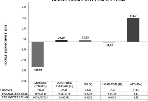
Once the tasks referring to the elaboration of the monthly mining plan were concluded, their execution begins. With the use of the estimated HPF, it was possible to evaluate the forecasted and executable parameters, as well as the impact of each of these parameters

on the hourly productivity. Figure 1 shows the EX40 excavator performance analysis during the month of September 2012. When analyzing its performance using Equation 1, for example, a 72 t/h total loss was identified. The operational moment and loading time were

Figure1 Parameter variation impact on the EX40

excavator’s hourly productivity.

Similar analyses were performed for each of the loading machines and transport vehicles in order to verify

the negative and positive deviations observed during the implementation of the mining plan for September, 2012.

Table 8 shows the productivity varia-tions, comparing estimated against real.

HOURLY PRODUCTIVITY ANALYSIS SEPTEMBER/2012

LOADING MACHINES TRANSPORT FLEET

EX21 EX22 EX27 PM25 PM26 PM27 EX40 EX41 EX42 EX43 EX44 LT03 TOTAL FLEET ₁ FLEET ₂ FLEET ₃ TOTAL

ESTIMATE 1199,6 1440,3 989,7 1083,0 1190,O 1329,0 1969,0 1873,0 1745,0 1633,0 1736,0 1476,0 1468,5 338,0 385,0 377,0 367

REAL 948,8 1278,8 1113,9 1149,6 1200,7 1182,1 1897,0 1750,9 1579,9 1492,9 1933,6 1381,8 1437,2 344,2 366,3 385,3 367

VARIATION

(%) 26% 13% -11% -6% -1% 12% 4% 7% 10% 9% -10% 7% 2,2% -2% 5% -2% 0,0%

Table 8 Estimated and real productivity when im-plementing the mining plan during the month of September, 2012.

Table 8 shows the variation between the estimated and actual productivity for the each transportation fleet and loading machines. The overall productivity of the loading machines is proportional to the number of hours that each equipment operated in September 2012 and shows a variations of 2,2%, but there was a high

variation between the loading equipments locally. There were constant interruptions in the operation of excavators EX21 and EX22 due to the high number of hours in operating. These failures affected the stability of the production cycle. There was a decrease in productivity of the front-end-loader PM27 by operational failures.

But some loading machines reached an actual productivity result better than the estimated. These equipments offset the negative deviations. While the deviation for the transportation fleet that occurred in fleets 1, 2 and 3 were balanced in a way that total productivity achieved the same value as estimated.

5. Conclusion

reduction of average loading down time (ADT); and 446.7 t/h because of a reduction in the ATD performed.

Even though the equation uses the principal variables related to productiv-ity in order to estimate it, other variables

that were not covered in this study using multivariate regression could have influence on the actual results of hourly productivity. Among these, can be listed: dump time of the transporta-tion vehicles and operatransporta-tional time for

the excavation equipment when dealing with harder rocks. It was necessary to limit the number of variables in order to guarantee a high number of correlations between the selected variables for the HPF estimates.

The possibility of being able to estimate hourly productivity indicators makes mining plans more realistic,

as-sertive and coherent with the equipment assigned to execute the loading and transport operations. Another benefit

227

6. References

BANKS, J., CARSON, J. S., NELSON, B. L., NICOL, D. M. Discrete-event system simulation, (3 ed.), International Edition, 2001. 594p.

BRANDÃO, R., TOMI, G. Metodologia para estimativa e gestão da produtividade de lavra. R.E.M – Revista da Escola de Minas, 75 n.64: 77-83, jan/mar 2011. CHARNET, R., FREIRE, C. A. L., CHARNET, E. M. R., BONVINO, H. Análise

de modelos de regressão linear: com aplicações, (2ª ed.)., Campinas: Editora da Unicamp, 2008. 356 p.

CHUNG, C. A. Simulation modeling handbook: a practical approach. CRC Press, USA, 2004. 504 p.

LAW, A. M. KELTON, W. D. Simulation modeling and analysis, (3a _ed.).

McGraw--Hill, 2000. 760 p.

ROBINSON, S. Simulation: The practice of model development and use. England : John Wiley & Sons, 2004. 316 p.

Received: 18 December 2012 - Accepted: 04 April 2014. between forecasted and executed

produc-tions. With the mapping of the bottle-necks identified through the comparison between the considered parameters in the estimate and reality, it is also possible to utilize management tools to control HPF. The multiple regression techniques are simple and affordable because there is software available to assist their ap-plication. These concepts can be used on monthly plans, weekly plans or even mining plans with larger time horizons. For the loading machines, the model

did not perform well locally presenting a high variance between 26% to -11%. But the final result, considering all of the equipment, was balanced in a way that total productivity achieved a value near reality. For the transportation fleet, the estimate informed actual productivity, without variation. This result shows that the integration of various equations obtained by multivariate regressions was efficient in estimating the productivity of the loading and transportation opera-tions of a determined mine.