PAPER
Recharge estimation from discrete water-table datasets in a coastal
shallow aquifer in a humid subtropical climate
Fabrizio Rama1&Konrad Miotlinski1&Davide Franco1&Henry X. Corseuil1
Received: 10 October 2017 / Accepted: 30 January 2018 #Springer-Verlag GmbH Germany, part of Springer Nature 2018
Abstract
A time-series approach to the estimation of recharge rate in unconfined aquifers of highly variable water level is proposed. The approach, which is based on the water-table fluctuation method (WTF), utilizes discrete water-level measurements. Other similar techniques require continuous measurements, which makes them impossible to apply in cases where no data from automatic loggers are available. The procedure is deployed at the Ressacada Farm site, southern Brazil, on a coastal shallow aquifer located in a humid subtropical climate where diurnal water-level variations of up to 1 m can follow a precipitation event. The effect of tidal fluctuations on the groundwater levels is analyzed using a harmonic component builder, while a time-variable drainage term is evaluated through an independent analysis and included in the assessment. The estimated recharge values are compared with those obtained from the continuous measurements showing a good agreement with the approaches for discrete dataset intervals of up to 15 days. Subsequently, the estimated recharge rates are incorporated into a transient groundwater-flow model and the water levels are compared showing a good match. Henceforth, the approach extends the applicability of WTF to noncontinuous water-level datasets in groundwater recharge studies.
Keywords Water-table fluctuation method . Groundwater recharge/water budget . Numerical modeling . Tidal influence . Brazil
Introduction
Accurate estimation of groundwater recharge is of relevance for different applications related to the assessment of human activity and hydrogeological characterization. It may be criti-cal information to manage changes in groundwater systems effectively (Xiao et al.2016) and to safeguard scarce resources in arid zones (de Vries and Simmers2002). Proper estimation of recharge and its variability in time and space is shown to be crucial for both the agricultural sector (Bohlke2002) and the assessment of fate and transport of solute pollutants (Kim et al. 2000), since it can induce temporal fluctuations in the flow field. Spatial and temporal variability in recharge, as well as
preferential flow paths, are key components for assessing aquifer vulnerability to a specific compound (Scanlon et al. 2002). Many investigators deal with the relationship between recharge estimation and numerical groundwater models (Colombani et al.2016; Sanford2002), focusing on the main role of vadose flow for simulating recharge (Cao et al.2016; Heilweil et al.2015). For a humid climate, Hunt et al. (2008) showed similar timing of recharge but an appreciably different water budget when considering thin unsaturated zones in the simulation. The literature reports a multitude of methods being developed and commonly used to infer recharge (Healy 2010). Recharge is part of the overall infiltration mechanism, when the wetting front reaches the water table, causing its rise. Precipitation is the main forcing of the process, and it is an important factor in the recharge estimation (Shi et al.2015). Theoretically, in a uniform porous medium with a shallow water table, it can be assumed that a fraction of total precipi-tation in a time step contributes to the aquifer recharge (Park and Parker2008), resulting in a prompt rise of water level in shallow unconfined aquifers (Hilberts et al.2007). The deeper the water table, the greater the amount of rainfall water held in the unsaturated zone, which in consequence leads to a reduc-tion of the precipitareduc-tion fracreduc-tion reaching the water table and
Electronic supplementary materialThe online version of this article (https://doi.org/10.1007/s10040-018-1742-1) contains supplementary material, which is available to authorized users.
* Fabrizio Rama
1 Department of Environmental Engineering, Federal University of
Santa Catarina (UFSC), Florianopolis, SC 88040-900, Brazil
to a time lag between the forcing and water-table rise. Realistically, estimation of groundwater recharge is an itera-tive process, involving multiple approaches with progressive aquifer-response data collection and resource evaluation (de Vries and Simmers2002). For this reason, despite this abun-dance of solutions, assessing the accuracy of any applied method (Healy and Cook2002) and choosing the most appro-priate for given field conditions (Scanlon et al.2002) is still extremely difficult.
The water-table fluctuation method (WTF) is a widely used method (Masetti et al.2016; Saghravani et al.2015) which requires the knowledge of groundwater levels to estimate re-charge. Usually applied in an event-basis framework (Delin et al.2007; Lorenz and Delin2007), WTF is a simple method applied for unconfined aquifers with a shallow water table and sharp variation in water level. There are three principal re-quirements for the use of WTF (Healy 2010; Healy and Cook 2002): (1) the applied time step must be as short as possible, (2) an accurate value of specific yield must be used (Acharya et al.2012; Nachabe2002), and (3) other possible causes of groundwater head fluctuations not related to re-charge must be isolated from the dataset (Neto et al. 2015). In order to estimate recharge useful for aquifer water-balance calculations, a time series approach for WTF has been devel-oped by Crosbie et al. (2005) showing a reliable and well-founded methodology. Nevertheless, its application for con-tinuous datasets presents two major limitations: (1) the empir-ical estimation for groundwater drainage by a linear function of depth may not properly explain the spatial and temporal variability of the flow field (Cuthbert2010), and (2) the model requires a continuous and homogeneous level dataset with sufficiently high temporal resolution, at least with hourly records.
Although hydrogeologists constantly deal with a lack of data, there is a tendency to neglect historical databases with incomplete and disjointed information. Nevertheless, discrete records of water-table depth can bring some useful informa-tion if they are treated using correct methodologies. This paper extends the application of the time series approach (Crosbie et al.2005) for discrete hydraulic head datasets. To address this issue, a variable drainage term (D term) may be intro-duced as an exponential function of the time elapsed from the last rain event, explaining water head reliance of discharge in the time domain. To verify the whole procedure, recharge estimates from a couple of piezometers are compared with those obtained from continuously monitored water-table se-ries and integrated in a transient 2D vertical flow model. In addition, a harmonic component analysis of high-frequency residual signals is included in the analysis to assess the astro-nomical tide influence on the groundwater levels in the area, excluding other processes responsible for water-table rises. This contribution aims to clarify the uncertainties in recharge estimates with WTF from discrete records and explains how to
extract useful groundwater information from irregular datasets.
Site description
An unconfined aquifer at the Ressacada Farm experimental site, in the southwestern part of Santa Catarina Island, south-ern Brazil, is studied (Fig.1a,b). The aquifer, 30–40 m thick, is fairly homogeneous consisting of lacustrine deposits with a predominance of fine quartz sand with lenses of silt and clay (De Lage2005). The total area is 20 km2and the aquifer is laterally adjacent to (1) an Atlantic channel called South Bay to the north and west (Garbossa et al.2014), (2) the slow curvy estuarine system of the Tavares River surrounded by man-grove swamps to the east, and (3) a compact granite complex of hills to the south (Fig.1c). The groundwater flow is a result of a very low natural gradient driven by precipitation recharge, and is radial diverging from the domain center to the boundaries.
The ground surface is flat (up to 5 m in elevation) and the average depth to water level varies from 0.3 to 2.0 m. The aquifer constitutes a u-shaped groundwater system (Huang et al.2015; Mao et al.2006) which is enclosed on three sides by natural surface water bodies subjected to boundary tidal fluctuations, carried by tidal channels and swamp dynamics. A dense network of artificial trenches in the plain drains the top of the shallow aquifer maintaining the water level below the topographic surface.
From a meteorological point of view, the region is located in the humid subtropical climate zone under the Köppen-Geiger classification (Peel et al.2006) at the contact of the Atlantic moist tropical and Antarctic polar air masses. The interactions and alternations between the fronts cause rainfall events with high intensity and large variability (Grimm et al. 1998). Precipitation is predominantly in the summer season, and the monitored annual rainfalls varied from 1,100 to 2,700 mm between years 2007 and 2017. The large variability of rainfall results in large and quick fluctuations of the ground-water levels.
highly conductive nature of the deposits; the intermittent, in-tense and spatially variable nature of rainfall; and the proxim-ity to boundary receptors. Experimental Area 3 is approxi-mately 3 km from South Bay, 2 km from Ribeirão Bay, and less than 500 m from the Tavares River; nevertheless, the area is located far away from intensive anthropogenic activities, with no pumping, and steep hydraulic gradients. For these reasons, the aquifer satisfies the conditions to apply the WTF for recharge estimations (Healy and Cook2002) which are: (1) lack of confinement with sharp temporal water-level changes; (2) large number of piezometers to observe water levels; (3) no pumping and no anthropogenic activities that may influence the natural groundwater level over short time scales; (4) a short time lag, and intense and variable rainfall events.
Materials and methods
Methodology
A discrete dataset of water levels from 13 piezometers mea-sured from 2007 to 2016 is used in the study (Table1). Most of the wells in the area are shallow piezometers that intercept the aquifer up to a depth of 4.5 m, with the exception of PZ01, PZ02 and PE06, which reach 15, 10 and 30 m in depth, re-spectively. Water-table depths were monitored with a manual phreatimeter at variable recording intervals (1–60 days). In
addition, in a shorter time window (from 8 February 2017 to 31 March 2017), PE03 and PM04 are equipped with automat-ic water-level loggers, recording every 15 min. Both wells are supplied with a vented pressure transducer of a range of 3.5 m with an accuracy of ±0.1%; therefore, the instruments auto-matically correct the measurements by pressure, to be vented, and by temperature deviation, with a linearizing algorithm of two known points; hence, the resulting total error is in the order of ±2 mm.
The WTF is based on the premise that water-table rises are due solely to vertical rainfall infiltration (Healy and Cook 2002); therefore, in a time step∆t, a total amount of recharge R[mm] is mathematically defined as:
R¼SyΔ h
Δt ð1Þ
whereSyis the specific yield [% by volume], and ∆his the maximum registered water-level change [mm] in a time step ∆t. A recharge ratio RR [%] is:
RR¼R
P ð2Þ
wherePis the total amount of rainfall [mm] in the same time step∆t. ThePrepresents total precipitation including events not contributing to water-level rises, whereasRrefers to the sum of all level rises in the same period. In accordance with Eq. (1), all the components in the groundwater budget that are not storage (like evapotranspiration, net subsurface flow or Fig. 1 Location of study area:amap of Brazil;bmap of Santa Catarina
Island;cstudy domain at Ressacada Farm Experimental Site, with boundary conditions. Section A–A′indicates the domain transect;d
Detailed map of Experimental Area No. 3, depicting: piezometer
baseflow) are supposed null during the recharge process. The time lag between the arrival of the infiltrated water and its redistribution to all the components is place-specific and de-termines the reasonable time step to be applied in the method. Therefore, over cumulative time intervals (months or years), all the contributions that are not accounted in the recharge term, like evapotranspiration losses and surface runoff during the precipitation, are lumped in (1-RR), with RR defined in Eq. (2). Using the WTF, recharge values are inferred in vari-able time steps along a time window of 10 years. A varivari-able drainage rate and variations ofSywith depth are included in the evaluation. The time series approach by Crosbie et al. (2005) is modified to handle discrete datasets with irregularly spaced data. This is to handle heterogeneity of datasets which made it difficult to directly compare one-by-one data using statistical methods available in the time-series analysis (Neto et al.2015).
The paper follows three main stages. In the first part, the recharge values are estimated on the basis of water-level fluc-tuations using a sparse, discontinuous and time-variable dataset with time intervals varying from 1 to 60 days. In the second part, the estimates are compared with the continuous time-series approach (Crosbie et al.2005). Finally, in order to verify the assumptions, test the conceptual model and calcu-late water balances, a numerical model was built with a finite element method (FEM), the FEFLOW code (Diersch2014).
Discrete-series approach
Discrete and irregularly spaced records of water-table levels are used to automate the estimation of monthly accumulated
recharge. In accordance with the work of Shi et al. (2015), which indicates precipitation as the most important factor con-trolling the daily and monthly WTF recharge estimates, the following conditions are applied in the approach:
RΔti¼ðΔhiþDΔtiÞ Sya →i f ∑ Δti
Pd
>0 and ðΔhiþDΔtiÞ>0 ð3Þ
where ∆hirepresents the ‘differenced water level’ in each interval [mm], that is the difference in water head between two consecutives records,Dis the drainage rate [mm/d] or D term,∆ti is the interval time length [d], Pdis the daily accumulated precipitation [mm], andSyais the apparent spe-cific yield [% by volume], estimated by Eq. (5). Subscripti represents all intervals available in the dataset; hence, the re-charge value in Eq. (3) is estimated in the rainy intervals solely, and is corrected by all drainage contributions lumped in theDterm, including the moisture content of the unsaturat-ed zone. The term substitutes, at each interval, the drawing of the Bantecedent recession curve^ that the well hydrograph would have followed in the absence of the rise-producing precipitation (Healy and Cook2002; Fig.2a), in analogy with the Master Recession Curve approach (Delin et al.2007).
The methodology is divided into five basic steps. Firstly, the series are synchronized and the measurements are consol-idated to remove errors or outliers. In order to avoid underes-timation of recharge (Delin et al.2007) sampling intervals longer than 15 days are excluded, losing only 1% of records; therefore, the resultant average sampling interval used in the procedure is 3–4 days. Secondly, the raw depth dataset is Table 1 Piezometers and their
design details Name
(Ref. code)
Ground elevationa, MSLb[m]
Well screen depth (top/bottom) [m]
Well screen elevationc, MSL (top/bottom) [m]
Well case diameter [cm]
PE01 2.83 2.5/4.5 0.3/–1.7 5.08
PE02 3.20 2.5/4.5 0.7/–1.3 5.08
PE03d 3.30 2.5/4.5 0.8/–1.2 5.08
PE06 3.10 20.0/30.0 −16.9/–26.9 10.16
PE07 2.72 11.0/13.0 −8.3/–10.3 11.43
PM01 3.32 2.5/4.5 0.8/–1.2 5.08
PM02 3.24 2.5/4.5 0.7/–1.3 5.08
PM04d 2.50 2.5/4.5 0.0/–2.0 5.08
PM05 3.32 2.5/4.5 0.8/–1.2 5.08
PM06 2.88 2.0/4.0 0.9/–1.1 5.08
PM18 2.66 1.0/3.0 1.7/–0.3 5.08
PZ01 3.12 10.0/15.0 −6.9/–11.9 5.08
PZ02 3.19 5.0/10.0 −1.8/–6.8 5.08
a
Ground elevation:values obtained with a Geodetc total station (distance accuracy of 5 mm and angular de 2″)
b
MSL:elevation above Mean Sea Level (zero reference at the ground control point of Imbituba Sea Level Station)
c
Well screen elevation:equal toGround elevationminusWell screen depth
d
converted to absolute hydraulic head above mean sea level. Thirdly, the difference in water levels between consecutive measurements (∆hi) is defined. Then, the amount of rainfall in each interval [mm] is calculated as the sum of the daily precipitation (Pd) between the first day and the second to last day of the interval as in Eq. (4).
PΔti ¼ ∑ Δti
Pd →if ∑ N−1
d¼1
Pd with ðΔti¼t1;t2;…;tNÞ ð4Þ
Finally, accumulated precipitation is used to divide the time-series: intervals with null accumulated precipitation are isolated and used to determine the rates related to the drainage processes where no recharge occurred, while intervals with positive accumulated precipitation are used to infer the re-charge itself.
As derived analytically by Cuthbert (2010) groundwater drainage in a flat unconfined aquifer is a transient function depending on the distance from (a) the surface receptor and (b) water-table head. The water head dependency of drainage (Dterm) in the Ressacada Farm site is explained as an empir-ical exponential function with respect to time for a period of 10 years (from 2007 to 2016; Rama et al.2017). Since a linear relationship between saturated volume and groundwater dis-charge at quasi-steady-state conditions was suggested (Walker et al.2015), it was proposed to group the rates into classes representing time elapsed since the last rain event. In order to simplify the procedure these averaged values are used in the
discrete approach of WTF to infer recharge. Thus, upper and lower drainage values in a significant time-scale obtained from the average best-fit curve for the whole area are as fol-lows: 12.7 mm/d for the low-head drainage of the aquifer in dry periods, and 57.7 mm/d immediately after a rainfall event, when the hydraulic head of the aquifer is high (Fig.2b). As shown in Fig.2b, low-head drainage indicates the water-table decreasing rate after 24 days with no rain, since dry periods never overstepped 25 days in 10 years of monitoring. In the continuous approach of WTF, a constantDterm is set up to 24 mm/d, equal to the median of the whole distribution of drainage rates.
An apparent specific yield (Sya) represents the storage of water controlled by capillary forces above the water table, assuming a transient nonideal release of water (Childs1960; Duke1972). Mathematically, for a layered soilSyais defined as (Crosbie et al.2005):
Syu ¼ðϕ−SrÞ → Sya¼Syu−
Syu
1þðαdÞn
½ 1−1n
ð5Þ
whereϕis the total porosity,Sris the specific retention, also known as field capacity [% by volume],dis the mean depth of the water table in the time step [cm], andSyuis the ultimate specific yield [% by volume]. To determine Syaa nonlinear relation between soil moisture and specific yield is assumed, supposing pressure distribution at equilibrium at each step. Given the spacing of the sampling intervals and a quick Fig. 2 Conceptual model sketches:a Definition of the WTF for
continuous (red arrows) and discrete (blue arrows) datasets:∆Hi
represents the total water-table rise in the interval, whereas∆hiis
defined according to the water-level measurements;bExponential model (equation) fitted on field data to assess theDterm as a function of the time elapsed since the last rainfall. Solid line is the mean function
reaction of the water table to the rainfall, this strategy seems reasonable.Syurepresents a steady specific yield without in-fluence of depth. Soil specific parameters of the Van Genuchten moisture model (α and n) are adopted from the Hanford sediment (Eching and Hopmans 1993) which ex-hibits similar characteristics and behavior with the Ressacada soil. In order to estimate Syu, the procedure by Armstrong and Narayan (1998) is automated for a discrete dataset, obtaining ultimate specific yield from the groundwa-ter level changes versus the accumulated precipitation plot (Fig.5). To assessSyu, only the water level declines in the last 50 cm of recorded depths in each piezometer are used. This corresponded to the water-table depth of at least 1.5 m; there-fore, only the low-head drainage value of 12.7 mm/d is ap-plied to lower records. Finally, multiplying the differenced water level series corrected with the drainage term by the Sya, the recharge in each interval is inferred and aggregated in a monthly recharge at the Ressacada farm.
Continuous analysis and tidal frequency analysis
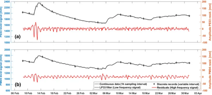
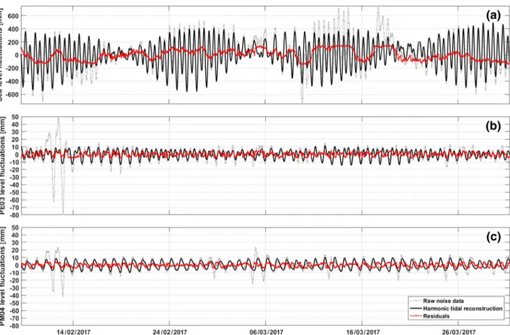
In the second stage, the discrete-series approach is compared with the continuous-series analysis proposed by Crosbie et al. (2005). The analysis is performed for the datasets PE03 and PM04 in a 51-day time window, from 8 February 2017 to 31 March 2017 (Fig.3), using both manually collected records (discrete and variably spaced data) as well as datalogger series (continuous and homogeneously spaced data). The two pie-zometers are chosen to be located along the main groundwater flow direction and exhibit the highest difference in the water-table variability.
To manage continuous datasets, water level records are firstly resampled to 1-h rate using a Doodson filter (Pugh 1987). This is followed by a data synchronization for the p e r i o d f r o m 8 F e b r u a r y 2 0 1 7 a t 1 5 : 0 0 : 0 0 t o 3 1 March 2017 at 09:00:00, to obtain 1,220 hourly records. In a congruence analysis, errors, spikes and noise are re-moved. To isolate periodic components with high frequen-cies, a Low Pass 33 filter (LP33) is subsequently applied (Emery and Thomson2001). Finally, in order to separate tidal influence from other periodic contributions (evapo-transpiration, atmospheric pressure variation, etc), a fre-quency analysis is carried out with a MATLAB-based UTide code (Codiga2011) on the residual signal (red lines in Fig.3). The harmonic component builder allowed one to identify the signal contribution at tidal frequencies from time series, including groundwater records. In addition, UTide is run on the sea level series, monitored in the South Bay, comparing the identified significant compo-nents with the PE03 and PM04 results. The significance of each component is attributed to the amplitude of the signal, based on the accuracy of the sensors and the signal-to-noise ratio (SNR) with a modified Rayleigh cri-terion, while their relative importance is controlled by the percent energy (PE) contributing to the signal reconstruc-tion (Codiga2011). The SNR value of 6 and a minimum PE of 0.5% are adopted. The sea levels in the South Bay are monitored by an OTT/RLS radar level sensor (accuracy of 3.5 mm, sampling frequency of 5 min) and are provided by EPAGRI/CIRAM (Agricultural Research and Extension C o m p a n y / I n f o r m a t i o n C e n t e r f o r E n v i r o n m e n t a l Resources and Hydrometeorology).
Fig. 3 Comparative plot of raw data (gray lines and diamonds), the Low Pass 33 filter signal (black line), and high frequencies residuals (red line) fora
Numerical FEM model
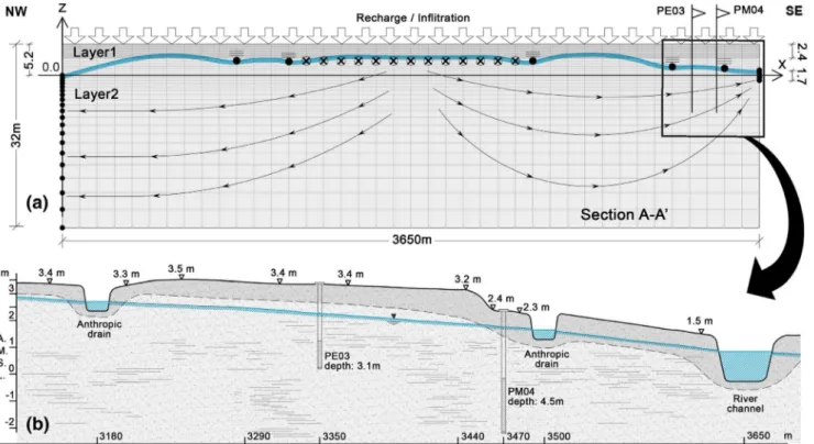
In the last stage, a 2D vertical finite element model is con-structed in order to integrate obtained recharge estimates in a transient simulation of the flow field. The model domain of 3,650 and 32 m in length and height, respectively, is divided into 18,154 rectangular elements (58 rows and 313 columns), regularly spaced in the horizontal direction every 11.7 m and with irregular spacing in the vertical di-rection. In the top 5.2 m of depth, the spacing is equal of 0.4 m and then increased gradually by about 5.5% until the bottom. The elevationz= 0 m refers to the mean average sea level. At the elevationz= 2.4 m the domain is divided into two layers of different hydraulic properties to reflect the existence of a superficial layer of finer geologic material rich in organic matter.
Constant-head boundary conditions (Dirichlet-type BC) are used to represent surface water bodies: South Bay on the left side (x= 0 m;z= 0 m), and Tavares River on the right (x= 3,650 m;z= 0.8 m). In addition, fiveBseepage face^BCs are introduced within the domain to represent partially pene-trating artificial ditches at an elevationz= 2.8 m (x= 944, 1,236 and 2,460 m), atz= 2 m (x= 3,180 m), and atz= 1.2 m (x= 3,500 m; Fig. 4). Conceptually, a seepage face corre-sponds to a constant-head BC, which is combined with a
maximum flux constraint equal to zero, allowing a free out-flow of water from the model. To reproduce a parallel trench influencing the flow field, but located outside of the simula-tion domain, a Cauchy flow BC constrained with a null max-flow rate is used (Diersch2014). This condition allowed for the performance of a distance-dependent drain in the central part of the domain from x= 1,294 m tox= 2,402 m at an elevationz= 3.4 m. Finally, recharge is represented by a fluid-flux BC on the top elements, which is a time-variable inflow condition. These values express volumes of water traveling through the unsaturated zone to the water table, solved by Richard’s Law and regulated by a modified van Genuchten moisture model. The details of the model set up are presented in Table2.
The model is calibrated using a trial-and-error method with the following criteria: (1) modeled hydraulic conductivity values should not deviate from the field-derived values by more than ±15%; (2) hydraulic conductivity values are adjust-ed for the steady-state comparing simulatadjust-ed levels with the average of monitored hydraulic heads; (3) the initial condition of hydraulic head for transient-state is obtained by a single calibrated steady-state run; (4) unsaturated-flow porosity of layer 1 for the transient-state should not deviate by more than ±15% from the average ofSyaestimates; (5) unsaturated-flow porosity of layer 2 and Richard’s model parameters are
Fig. 4 aTwo-dimensional (2D) finite element model setup along section A–A′(Fig.1c), used to test the recharge estimation methodology in stage 3. Filled dots represent the head boundary condition (BC), dots with lines above are constrained-head BC (seepage face), encircled crosses indicate Cauchy-type BC with flow constraint, lines with arrows show
adjusted using a fixed RR into the range established with the WTF estimates in PM04 and PE03, equal to 43% of moni-tored precipitation (Table3; Fig.7); (6) daily recharge values in transient-state must not exceed precipitation; (7) approxi-mation of hydraulic heads never oversteps minimal targets of 0.85 for the Nash-Sutcliffe (NS) efficiency coefficient, 10% of total observed head range for root-mean-square error (RMSE), and 10 cm of absolute error in comparison to field data (Anderson et al.2015).
Therefore, once the model results satisfactorily represent transient hydraulic head data, scenarios with different re-charge are constructed:
1. Recharge equal to 43% of daily precipitation, statistically
inferred from rainfall records, and input parameters in compliance with Table2 (also known as Bcalibrated scenario^)
2. Recharge assessed with the continuous-series method of
WTF (section‘Discrete-series approach’)
3. Steady constant recharge equal to 2.15 mm/d (43% of
average precipitation in the 51-day period)
4. Recharge equal to 43%, with a constant unsaturated-flow
porosity for the whole domain, equal to 0.188 (measure of Syuestimated as the inverse of the slope of the line of best fit in Fig.5)
Results and discussion
Recharge estimation by the discrete and continuous
approach to WTF
The water-level variations versus accumulated rainfall for each interval show a linear correlation (Fig.5). The inverse of the slope of the fitting line in the graph gives the value of Syuequal to 0.188 (95% confidence bounds from 0.185 to 0.192), which agrees with the field Syassessment (Corseuil et al.2011b).
All water losses (i.e. soil moisture variation, evapo-transpiration and run-off) are assumed to be included in the part of the rainfall that falls below the threshold value (x-intercepting value in blue Fig. 5). This means that on average only accumulated precipitation above 3.1 mm (2.5–3.7 mm with 95% confidence interval) has an evident influence on the Ressacada groundwater levels.
Table 2 The two-dimensional FEM model input parameters and conditions
FEM parameter Symbol Value [unit] Reference
Model parameters forBcalibrated scenario^
Saturated conductivity K 3.2 (layer 1)/8.5 (layer 2) [m/d] De Lage (2005)/field data Unsaturated flow porosity ε 0.067 (layer 1)/0.13 (layer 2) [−] WTF estimation/calibration
Specific storage coeff. S0 0 Diersch (2014)
Maximum saturation ss 1
Residual saturation sr 0.25 WTF method/field data
Modified van Genuchten parametric model
Pore-size distribution index n 2.2 [−] Diersch (2014) Fitting coefficient α 2.8 [1/m]
Fitting exponent m 0.55 [−] Fitting exponent δ 1 [−]
FEM - 2D mesh consisting of 18,154 quadrangle elements (313 × 58)
Domain XvsZ 3650 vs 32 [m] Conceptual model
Vertical space increment Δz 0.4 + (5.5%Δzi–1)[m]
Horizontal space increment Δx 11.661 [m] Initial time-step size Δt0 0.001 [d] RMS error tolerance (AB/TR) ξ 0.001 [−] Simulation time period tend 52 [d]
FEMfinite element method model, design by the FEFLOW code (DHI);RMSroot mean square
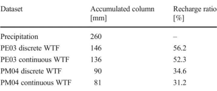
Table 3 Comparison between discrete and continuous dataset estimations within the 51-day period
Dataset Accumulated column [mm]
Recharge ratio [%]
Precipitation 260 –
PE03 discrete WTF 146 56.2
PE03 continuous WTF 136 52.3
PM04 discrete WTF 90 34.6
The estimates of average monthly recharge for the whole area show an outstanding variability (Fig.6). There is no constant or directly proportional relation between monthly precipitation and recharge which has a three-fold explana-tion: firstly, in rainy months the intense runoff, due to the temporal proximity of precipitation events to each other, has less contribution to a water-table rise; secondly, recur-rent flooding events during the intense precipitation periods reduces groundwater recharge; finally, swamp areas near the Tavares River modify hydraulic head to boundary re-ceptors for long periods resulting in a reduced capacity for aquifer drainage, and hence, storage capacity. It should be highlighted that, since months with no available water level records are excluded from the analysis, no bar of recharge is shown in the graph for these months. For the discrete dataset of 13 piezometers the total recharge in 10 years varies from 5,634 to 6,957 mm which constitutes from 38.5 to 47.2% of precipitation, respectively; this is on av-erage 43% of RR in the area (Fig.7).
The values of monthly recharge sums indicate that average annual recharge varies between 536 to 885 mm/year, respec-tively, for the driest and wettest year, whereas the annual re-charge range (difference between maximum and minimum value) between all the piezometers is on average 230 mm. Therefore, average recharge ratios are in the range of 35.9– 51.6%, resulting in a wider range of RR than the 10-year analysis; additionally, it should be emphasized that the years
with more accumulated rainfall show the lower RR values. This suggests that the effectiveness of recharge decreases with the increase of precipitation, due to an enhanced saturation of pores; an effect widely referred to asBfill and spill^systems (Tromp-van Meerveld and McDonnel2006). The implication is that dry winter months show on average markedly higher RR, whereas during the rainy months RR is lower.
Recharge estimates for the continuous datasets during a 51-day time span are 136 and 81 mm for PE03 and PE04, respectively. The recharge estimates in the same period for the discrete datasets are 146 and 90 mm for PE03 and PE04, respectively, showing a good agreement between the ap-proaches (Table3).
The sensitivity analysis of inferred recharge ratios (RRs) to the model parameters is summarized in Table4. In the column headings, RRs in parentheses refer to the whole 10-year time period for the different Syuvalues andDterm. The recharge estimates with WTF exhibit a linear relationship withSyu val-ue, as shown in Eq. (5). Nevertheless, ifSyuis constant (noSya decline at the surface) recharge estimates increase dramatically, which is an observation that confirms the finding by Child (1960), indicating an overestimation of recharge if a constant Syis used instead of a non-steady value. In addition, the model seems to be very sensitive to the drainage term, highlighting the importance of its accurate assessment. The Dterm has increasing influence depending on the larger time step between the records. Similarly, uncertainties on the real recession Fig. 5 Ultimate specific yield
estimation using the regression best fit (red line and equation) in a precipitation vs water-table fluctuation plot. R2adj is the
degree-of-freedom adjusted coefficient of determination for the typed equation. Dotted lines show the prediction interval for a non-simultaneous new
hydrograph intensify their relevance in the final estimation; thus, for this reason, the authors suggest to use head-variable Dvalues up to 1 week, adopting a fixed low-head or medianD value for time intervals overstepping 1 week.
Integration of WTF results into the FEM model
Observed and simulated water head values in PM04 and PE03 show a good agreement (Fig.8), with a NS coefficient of 0.87 and a RMSE of 5 cm. Solid lines in the graph represent cali-brated simulation with parameters as in Table2and RR equal to 43% of daily precipitation (scenario 1). Recorded precipi-tation and water-table variation (dashed lines) indicate a gen-erally fast response of the Ressacada aquifer to infiltration forcing (8–24 h). The distribution of simulated levels (solid lines) indicates a similar timing in recharge in agreement with findings by Hunt et al. (2008). In addition, the comparison of Fig. 6 Comparative bar plot between monthly recharge estimates (light bars) and total precipitation (dark bars). Recharge bars are average values between the 13 piezometers
Fig. 7 Statistics boxplot of estimated recharge ratio (RR) for different time periods. Red lines express median value of distribution; blue boxes indicate the 25th and 75th percentiles, while dashed whiskers extend to the most extreme data points. Red dashed line show 43% (median RR in 10 years)
Table 4 Summary of sensitivity analysis results
Syu(RR)a
[% by volume]
Dterm (RR)a [mm/d]
0.188 (0.430) 0.13 (0.302) 0.2 (0.464) 0.2 constantb(0.794)
Initial values: 12.7–57.7c(0.430)
Constant low-head value: 12.7 (0.357) No correction withDterm: (0.248) Constant average value: 20.7 (0.441) Higher piezometer: 15.2–66.2c(0.483) Lower piezometer: 9.6–35.9c(0.390)
a
RRin brackets is the average recharge ratio between all piezometers, calculated as the ratio of total recharge in 10 years and total accumulated precipitation
b
Constant specific yield equal to field assessment (Corseuil et al.2011b)
c
records from two piezometers exhibits greater distance be-tween the two lines during a rainfall event and immediately after it, with a scarce increase of PM04 levels compared with levels at PE03. This behavior demonstrates the spatially dif-ferent recharge in the area, with greater fluctuations in areas further away from the boundary receptors.
The numerical model allows one to compare water budget components between the estimated recharge with WTF and different FEM scenarios. Comparative analysis of the water columns at the end of the simulation (Fig.9) shows a good agreement in the water budgets with the WTF estimates (Table3). Although the NS coefficient on the water-table head decreases from 0.87 to 0.76 passing from scenario 1 to scenario 2—see the electronic supplementary material (ESM)—water volumes at the end of the simulation are very close in both runs. It suggests that prior estimation of re-charge with WTF prevents a long trial-and-error process to assess the recharge with the numerical model, also providing a robust theoretical basis for its values. The difference in the shapes of theBrainfall recharge^curves (Fig.9) emphasizes that effectiveness of recharge is related to the precipitation distribution: first, a more intensive rainfall event (days 4–6) has less estimated RR than 43% and the curve grows less, whereas the second event (days 25–31), less rainy and more distributed in time, exhibits a higher RR than the average value of 43%.
The calibrated scenario 1 was also tested using a transient unsaturated flow porosity in layer 1 equal to the estimatedSya, as described in section‘Discrete-series approach’(seeESM).
Here, the water budget exhibits sharper curves in response to changing parameters along the simulation, with a higher con-tribution of storage volume to flow between days 9 and 25. Nonetheless, the total approximation of simulated levels re-sults in a NS coefficient of about 0.77. It should be highlighted that the storage contribution to flow at the end of 51 days remains similar in all the scenarios, except with a constant unsaturated-flow porosity equal toSyu(scenario 4). By run-ning this scenario (see ESM), hydraulic levels, and hence, water discharge budgets show a pronounced sensitivity to the parameter, with a drastic mismatch in the peak of hydrographs (absolute error more than 15 cm), although the simulation NS efficiency coefficient remains about 0.8. This explains the sensitivity of recharge estimates using WTF to the value of Syu (Table 4). Finally, by running the Bsteady recharge^run (scenario 3), simulated steady-state levels con-verge to the average of the transient hydraulic head in scenario 1, with also good agreement in the entire water budget at the end of the simulation (seeESM).
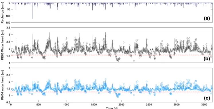
Using scenario 1, model verification is run on a 10-year-long discrete dataset of groundwater levels for PE03 and PM04 (Fig.10). The resulting water table shows a good model agreement for the majority of water level values, except for low water levels for which modeled values are overestimated. The head-BC assigned on Tavares River is meant to represent a natural dynamic system with sharp level fluctuations over time. In accordance with the head-dependent relationship of Darcy’s Law, the BCs define in the model the hydraulic gra-dient for nodes where flow occurs, mostly in long periods Fig. 8 Combined plot showing water level fluctuations in the 51-day
period. Dashed lines represent continuously monitored piezometer levels, while solid lines are the calibrated asset (scenario 1). The bar
without rainfall. This behavior implicates a progressively slower flow as the water table approaches an equilibrium state with the BCs; however, dry periods determine lower levels in the river too, resulting in a faster decrease of groundwater levels in the field, which are impossible to simulate with fixed values of BCs. Therefore, the authors suppose that the devia-tion could be reduced with the use of a time-variable boundary condition at the river cells rather than a time-constant value;
nevertheless, the deviation from the field data occurs in pe-riods of null recharge only, and, hence, it is of a low signifi-cance for long-term recharge estimation.
Tidal influence assessment
Frequency decomposition of the groundwater-level sig-nals indicates an only marginal tidal influence on PE03
Fig. 10 2D model verification plot: comparison between simulated (solid lines) and monitored levels dataset (symbols) in a 10-year-long simulation that used calibration parameters, forarecharge,bPE03,c
PM04. The red dashed lines (lower head value reached by simulation in
each piezometer) show that simulated lines never decrease under fixed values related to the river BC, losing accuracy to explain low groundwater levels
and PM04 hydraulic head in comparison to the other ape-riodic forcings, like rainfall infiltration (Fig. 3). In fact, the absolute value of the reconstructed signals remains confined within 12.2 mm (sygizial tides) and −9 mm (quadrature tides). Nevertheless, analysis of harmonic components on the high frequency residuals allows a quantitative assessment of tidal influence on PE03 and PM04 hydraulic head.
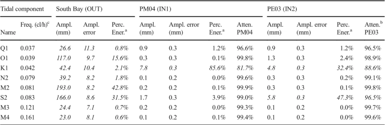
Since the tide estimation uses a 51-day time series, 35 harmonic components are identified. However, when apply-ing significance limits (SNR = 6 and PE > 0.5%), only eight of those components are shown to be relevant in the South Bay signal and only two in the groundwater level records. Astronomical tide assessment on the South Bay shows that 73.6% of the sea level records are explained by high-frequency periodic contribution, while the other 26.4% is due to other meteorological forcings. In the same way, astro-nomical tide components explain 33.2 and 49.9% of residual signals after LP33 application, on PE03 and PM04, respec-tively (Fig.11). It should be noted that PM04 is 180 m away from the river channel, while PE03 is 300 m away (Fig.4).
This fact indicates a higher percentage of tidal influence on the signal of the closest piezometer to the river and suggests
that only a small part of the tidal perturbation in the South Bay influences water head in the inland piezometers. Most of higher frequency components seem to be smoothed out by pressure propagation in porous media, in accordance with the main theory of incompressible flow: the higher the com-ponent frequency, the greater the attenuation in a dissipative media.
In addition, comparative analysis on K1, that is the only relevant component greater than sensors accuracy (Ampl ≥ 3.5 mm) in both PE03 and PM04, indicates that perturbations decrease moving inwards (Tables 5 and 6). PE03 showed an attenuation rate higher than PM04, which conserves more amplitude. At the same time, the PE03 signal had more phase delay than PM04. This observation confirms the findings of Mao et al. (2006) and is due to the tidal perturbation path-way, which moves from the estuary along the course of the river toward the center of the domain. Nevertheless, other nonrelevant components (S2 and O1) exhibit an opposite behavior, which may be due to an additional interaction of the PM04 signal with the water level in the artificial trench close by, where no tidal effects are observed.
Fig. 11 Signal reconstruction by harmonic components ofaSouth Bay seawater level monitoring, and thebPE03 andcPM04 high frequency signal. In each graph a comparison of raw high frequencies records (gray
Conclusions
The paper describes the use of a time-series approach for WTF, with discrete and irregularly spaced water-level datasets. The application of WTF allowed for the estimation of the groundwater recharge from sparse head records in an aquifer with a shallow water table and sharp fluctuations. The methodology represents an improvement on WTF, increasing its application possibilities. The introduction of a time-variable drainage term and the definition of the differenced water levels based on monitored precipitation allowed for the moderation of the the recharge underestimation with in-creasing time steps. Hence, the results in the 51-day time
window show good agreement with the results of the Crosbie et al. (2005) method. For the water-level dataset be-tween 2007 and 2017, the estimated amount of recharge is on average 43% of precipitation, showing a higher effectiveness of recharge in theBdry^months with less accumulated rain-fall. Subsequently, estimated recharge values are integrated into a 2D finite element model that agrees with observed water level records. Solely low water levels are overestimated in the simulation, probably due to the constant-head BC in the river, suggesting the possibility to introduce a variable-in-time con-dition to better reproduce dry periods with deeper water table. The application of WTF is limited to changes in ground-water levels over time due to rainfall infiltration only. This Table 5 Comparative tidal analysis (amplitudes with 95% confidence interval). Values initalicare the relevant components (namely SNR≥6, PE≥0.5%, and Ampl.≥3.5 mm)
Tidal component South Bay (OUT) PM04 (IN1) PE03 (IN2)
Name
Freq. (cl/h)c Ampl.
(mm)
Ampl. error
Perc. Ener.a
Ampl. (mm)
Ampl. error (mm)
Perc. Ener.a
Atten. PM04
Ampl. (mm)
Ampl. error (mm)
Perc. Ener.a
Atten.b
PE03
Q1 0.037 26.6 11.3 0.8% 0.9 0.3 1.2% 96.6% 0.9 0.3 1.2% 96.5%
O1 0.039 117.0 9.7 15.6% 0.3 0.3 0.1% 99.8% 1.3 0.3 2.4% 98.9%
K1 0.042 42.4 10.4 2.1% 7.8 0.3 85.6% 81.7% 4.8 0.3 32.4% 88.6%
N2 0.079 39.2 8.2 1.8% 0.1 0.2 0.0% 99.6% 0.3 0.3 0.2% 99.1%
M2 0.081 193.0 8.2 42.8% 0.2 0.2 0.1% 99.9% 0.3 0.3 0.1% 99.8%
S2 0.083 166.0 8.6 31.5% 1.7 0.3 3.9% 99.0% 5.8 0.3 47.3% 96.5%
M3 0.121 24.4 7.1 0.7% 0.2 0.2 0.0% 99.3% 0.1 0.2 0.0% 99.7%
M4 0.161 23.0 8.1 0.6% 0.1 0.2 0.1% 99.4% 0.1 0.2 0.0% 99.6%
a
Perc. Ener.is the percent of energy (PE) that contributes to the signal reconstruction as the ratio between component energy, gauge of potential energy of
sea level, and total energy of the reconstructed signal
b
Atten.is the attenuation of the component in comparison of the South Bay signal. It is calculated by 100 minus the ratio of component amplitude in the
piezometer and in the sea-level gauge
c
cl/hmeans cycles per hour. It is a frequency unit that implies a 1/3600 cl/h for a frequency of 1 hertz
Table 6 Comparative tidal analysis (phases with 95% confidence interval). Values initalicare the relevant components
Tidal component South Bay (OUT) PM04 (IN1) PE03 (IN2)
Name Freq. (cl/h)
Pha (360°)
Pha error
SNR (RM)a
Pha (360°)
Pha error
SNR (RM)a Δ
Phab
PM04 (h) Pha (360°)
Pha error
SNR (RM)a Δ
Phab
PE03 (h)
Q1 0.037 56 21 22 159 22 34 −7.7 273 22 29 −16.2
O1 0.039 73 5 560 191 81 3 −8.5 347 15 73 −19.6
K1 0.042 150 13 64 166 2 2300 −1.1 221 4 780 −4.7
N2 0.079 145 13 89 359 417 2 −7.5 96 44 6 1.7
M2 0.081 79 3 2100 172 58 5 −3.2 145 58 5 −2.3
S2 0.083 83 3 1400 122 10 150 −1.3 99 9 1700 −0.5
M3 0.121 174 18 46 99 82 1 1.7 223 158 1 −1.1
M4 0.161 99 21 31 276 95 3 −3.1 113 147 1 −0.2
a
SNR (RM): signal-to-noise ratio with modified Rayleigh criterion
b
condition is confirmed to be reasonable at the Ressacada Farm site, by analyzing tidal influence on groundwater levels and absolute values of the residual high-frequency signal in the piezometers, which was usually less than 2 cm of amplitude. Since WTF was shown to be very sensitive to the specific yield, its value is assessed in the paper with a statistically based framework that integrates punctual field measures. The main requirement of the proposed procedure is to allocate all the accumulated precipitation of each interval to the last day of the interval, as if total rainfall infiltrates and recharges the aquifer at the same time. As the sampling intervals in-crease, the underestimation of recharge using the cumulative approach increases. This limitation is mitigated by introducing a variableDterm to account for the water volume that leaves the aquifer in the same time interval. Finally, another impor-tant issue is related to the representativeness of the catchment as a whole. The uniform geological setting made the extrapo-lation of the relevant processes outside of the head monitoring area possible. Nonetheless, it is warranted to incorporate data from outside of the farm site, most of all in the center of the domain, in order to establish representative values for the watershed.
Acknowledgements The authors want to acknowledge FEESC and Petróleo Brasileiro (Petrobras) for the material support that made this study possible and DHI Group for providing aMIKE Powered by DHI
license file to use FEFLOW. We thank also the Institute of Airspace Control (ICEA) and National Institute of Meteorology (INMET) for pro-viding valuable precipitation data, all the technicians of Agrarian Sciences Center (CCA) for their support in the field data collection, Dr. Luis H. P. Garbossa for help obtaining sea-level records from the EPAGRI/CIRAM gauge station in the South Bay, and the PhD student Martina Pacifici (USP, PPGEC) for help in figure design. Finally, the manuscript benefited from suggestions from two anonymous reviews and comments/discussions with Sue Duncan (technical editorial advisor
ofHydrogeology Journal) for which we are most grateful.
Funding Information Additionally, the authors acknowledge FEESC and Petróleo Brasileiro (Petrobras) for the financial support that also made this study possible.
References
Acharya S, Jawitz JW, Mylavarapu RS (2012) Analytical expressions for drainable and fillable porosity of phreatic aquifers under vertical fluxes from evapotranspiration and recharge. Water Resour Res 48:1–15.https://doi.org/10.1029/2012WR012043
Anderson MP, Woessner WW, Hunt RJ (2015) Applied groundwater modelling, 2nd edn. Elsevier, Amsterdam, 564 pp
Armstrong D, Narayan K (1998) Using groundwater responses to infer recharge. CSIRO, Canberra, Australia
Bohlke J-K (2002) Groundwater recharge and agricultural contamination. Hydrogeol J 10:153–179. https://doi.org/10.1007/s10040-001-0183-3
Cao G, Scanlon BR, Han D, Zheng C (2016) Impacts of thickening un-saturated zone on groundwater recharge in the North China plain. J Hydrol 537:260–270.https://doi.org/10.1016/j.jhydrol.2016.03.049 Childs EC (1960) The nonsteady state of the water table in drained land. J
Geophys Res 65:1–3
Codiga DL (2011) Unified tidal analysis and prediction using the UTide MATLAB functions. Technical report 2011-01, Graduate School of Oceanography, University of Rhode Island, Narragansett, RI, 59 pp. ftp://www.po.gso.uri.edu/pub/downloads/codiga/pubs/2011Codiga-UTide-report.Pdf. Accessed 5 March 2017
Colombani N, Di Giuseppe D, Faccini B et al (2016) Inferring the inter-connections between surface water bodies, tile-drains and an uncon-fined aquifer–aquitard system: a case study. J Hydrol 537:86–95. https://doi.org/10.1016/j.jhydrol.2016.03.046
Corseuil HX, Monier AL, Fernandes M et al (2011a) BTEX plume dy-namics following an ethanol blend release: geochemical footprint and thermodynamic constraints on natural attenuation. Environ Sci Technol 45:3422–3429.https://doi.org/10.1021/es104055q Corseuil HX, Monier AL, Fernandes M et al (2011b) BTEX plume
dy-namics following an ethanol blend release: geochemical footprint and thermodynamic constraints on natural attenuation–supporting information. Environ Sci Technol 23.https://doi.org/10.1117/1111. 2794018.2
Corseuil HX, Gomez DE, Schambeck CM et al (2015) Nitrate addition to groundwater impacted by ethanol-blended fuel accelerates ethanol removal and mitigates the associated metabolic flux dilution and inhibition of BTEX biodegradation. J Contam Hydrol 174C:1–9. https://doi.org/10.1016/j.jconhyd.2014.12.004
Crosbie RS, Binning P, Kalma JD (2005) A time series approach to inferring groundwater recharge using the water table fluctuation method. Water Resour Res 41:1–9.https://doi.org/10.1029/ 2004WR003077
Cuthbert MO (2010) An improved time series approach for estimating groundwater recharge from groundwater level fluctuations. Water Resour Res 46, W09515.https://doi.org/10.1029/2009WR008572 de Vries JJ, Simmers I (2002) Groundwater recharge: an overview of
process and challenges. Hydrogeol J 10:5–17.https://doi.org/10. 1007/s10040-001-0171-7
Delin GN, Healy RW, Lorenz DL, Nimmo JR (2007) Comparison of local- to regional-scale estimates of ground-water recharge in Minnesota, USA. J Hydrol 334:231–249.https://doi.org/10.1016/j. jhydrol.2006.10.010
Diersch H-JG (2014) FEFLOW: finite element modeling of flow, mass and heat transport in porous and fractured media. Springer, Heidelberg, Germany, 996 pp
Duke HR (1972) Capillary properties of soils: influence upon specific yield. Trans ASAE 15:688–691
Eching SO, Hopmans JW (1993) Optimization of hydraulic functions from transient outflow and soil water pressure data. Soil Sci Soc Am J 57:1167–1175
Emery WJ, Thomson RE (2001) Data analysis methods in physical oceanography, 2nd edn. Elsevier, Amsterdam
Garbossa LHP, Vanz A, Fernandes L, et al. (2014) Modelling and valida-tion of the Santa Catarina Island bays hydrodynamics based on as-tronomic tides and measured tides. 11th Int. Conf. Hydroinformatics 8.https://doi.org/10.13140/2.1.5123.6163
Grimm AM, Ferraz SET, Gomes J (1998) Precipitation anomalies in southern Brazil associated with El Niño and La Niña events. J Clim 11:2863–2880. https://doi.org/10.1175/1520-0442(1998) 011<2863:PAISBA>2.0.CO;2
Healy RW (2010) Estimating groundwater recharge. Cambridge University Press, Cambridge, 245 pp. Available athttps://www.cambridge.org/ core/terms.https://doi.org/10.1017/CBO9780511780745.001. Accessed 12 September 2017
Healy RW, Cook PG (2002) Using groundwater levels to estimate re-charge. Hydrogeol J 10:91–109. https://doi.org/10.1007/s10040-001-0178-0
Hilberts AGJ, Troch PA, Paniconi C, Boll J (2007) Low-dimensional modeling of hillslope subsurface flow: relationship between rainfall, recharge, and unsaturated storage dynamics. Water Resour Res 43: 1–14.https://doi.org/10.1029/2006WR004964
Huang FK, Chuang MH, Wang GS, Der Yeh H (2015) Tide-induced groundwater level fluctuation in a U-shaped coastal aquifer. J Hydrol 530:291–305.https://doi.org/10.1016/j.jhydrol.2015.09.032 Hunt RJ, Prudic DE, Walker JF, Anderson MP (2008) Importance of unsaturated zone flow for simulating recharge in a humid climate. Ground Water 46:551–560. https://doi.org/10.1111/j.1745-6584. 2007.00427.x
Kim K, Anderson MP, Bowser CJ (2000) Enhanced dispersion in ground-water caused by temporal changes in recharge rate and lake levels. Adv Water Resour 23:625–635. https://doi.org/10.1016/S0309-1708(99)00050-0
Kobiyama M, Bortolotto NL, Tanaka SI (2011) Relatório Hidrológico da Fazenda experimental da Ressacada [Hydrological report of the Ressacada Experimental Farm]. Centro de Ciências Agrárias, UFSC, Florianópolis, Brazil. Available athttp://fazenda.ufsc.br/ descricao-fisica/hidrologia/. Accessed 1 October 2017
De Lage IC (2005) Avaliação de metodologias para determinação da permeabilidade em meios porosos: Fazenda Ressacada [Evaluation of methodologies for determination of permeability in porous media: Ressacada Farm]. MSc Thesis, UFRJ, Rio de Janeiro, Brazil Lorenz DL, Delin GN (2007) A regression model to estimate regional
ground water recharge. Ground Water 45:196–208.https://doi.org/ 10.1111/j.1745-6584.2006.00273.x
Mao X, Enot P, Barry DA et al (2006) Tidal influence on behaviour of a coastal aquifer adjacent to a low-relief estuary. J Hydrol 327:110– 127.https://doi.org/10.1016/j.jhydrol.2005.11.030
Masetti M, Pedretti D, Sorichetta A et al (2016) Impact of a storm-water infiltration basin on the recharge dynamics in a highly permeable aquifer. Water Resour Manag 30:149–165.https://doi.org/10.1007/ s11269-015-1151-3
Nachabe MH (2002) Analytical expressions for transient specific yield and shallow water table drainage. Water Resour Res 38(10):1193. https://doi.org/10.1029/2001WR001071
Neto DC, Chang HK, van Genuchten MT (2015) A mathematical view of water table fluctuations in a shallow aquifer in Brazil. Groundwater 54:82–91.https://doi.org/10.1111/gwat.12329
Park E, Parker JC (2008) A simple model for water table fluctuations in response to precipitation. J Hydrol 356:344–349.https://doi.org/10. 1016/j.jhydrol.2008.04.022
Peel MC, Finlayson BL, McMahon TA (2006) Updated world map of the Köppen-Geiger climate classification. Hydrol Earth Syst Sci 15: 259–263.https://doi.org/10.1127/0941-2948/2006/0130
Pugh DT (1987) Tides, surges and mean sea level. Wiley, Swindon, UK Rama F, Franco D, Corseuil HX (2017) Spatial and temporal analysis of natural drainage in the Ressacada aquifer (Florianopolis, Brazil). IJESD 8(9):653–660.https://doi.org/10.18178/ijesd.2017.8.9.1033 Saghravani SR, Yusoff I, Wan Md Tahir WZ, Othman Z (2015)
Comparison of water table fluctuation and chloride mass balance methods for recharge estimation in a tropical rainforest climate: a case study from Kelantan River catchment, Malaysia. Environ Earth Sci 73:4419–4428.https://doi.org/10.1007/s12665-014-3727-2 Sanford W (2002) Recharge and groundwater models: an overview.
Hydrogeol J 10:110–120. https://doi.org/10.1007/s10040-001-0173-5
Scanlon BR, Healy RW, Cook PG (2002) Choosing appropriate tech-niques for quantifying groundwater recharge. Hydrogeol J 10:18– 39.https://doi.org/10.1007/s10040-001-0176-2
Shi X, Vaze J, Crosbie R (2015) The controlling factors in the daily and monthly groundwater recharge estimation using the water table fluc-tuation method [online]. In: 36th Hydrology and Water Resources Symposium: The Art and Science of Water. ACT, Barton, Australia. h t t p : / / s e a r c h . i n f o r m i t . c o m . a u / d o c u m e n t S u m m a r y d n = 824177714642772;res=IELENG. Accessed1 October 2017 Tromp-van Meerveld HJ, McDonnell JJ (2006) Threshold relations in
subsurface stormflow: 2. the fill and spill hypothesis. Water Resour Res 42:W02411.https://doi.org/10.1029/2004WR003800 Walker GR, Gilfedder M, Dawes WR, Rassam DW (2015) Predicting
aquifer response time for application in catchment modeling. Groundwater 53(3):475–484.https://doi.org/10.1111/gwat.12219 Xiao H, Wang D, Hagen SC, et al (2016) Assessing the impacts of