MASTER
ACTUARIAL SCIENCES
MASTER´S FINAL WORK
DISSERTATION
OPTIMAL REINSURANCE OF DEPENDENT RISKS
ALEXANDRA BUGALHO DE MOURA
MASTER
ACTUARIAL SCIENCES
MASTER´S FINAL WORK
DISSERTATION
OPTIMAL REINSURANCE OF DEPENDET RISKS
ALEXANDRA BUGALHO DE MOURA
SUPERVISION:
P
ROFESSORM
ARIA DEL
OURDESC
ENTENOAcknowledgments
Firstly, I would like to thank Professor Maria de Lourdes Centeno for the supervision of this Thesis and for introducing me to the field of Actuarial Sciences. I specially thank her for the fruitful discussions and incentive in the final stage of this work.
I would also like to express my gratitude to all Professors of the Master in Actuarial Sciences, who contributed for my interest and knowledge development in this field.
I am very grateful to my parents and brothers for supporting my decisions and being always there, even when they are in different countries and continents. I thank my mother the constant availability with the kids.
Abstract
This Thesis focuses on the optimal reinsurance problem for two dependent risks, from the point of view of the ceding insurance company. We assume that the two risks are dependent by means of a copula structure. By risk we mean a line of business, a portfolio of policies or a policy.
The problem consists in finding the optimal combination of quota-share and stop loss treaties, for each risk, that maximizes the expected utility or the adjustment coefficient of the total wealth of the insurer. It is known that these two criteria are connected and moreover the adjustment coefficient is related to the ultimate probability of ruin of the insurer through
the Lundberg inequality. Results are obtained numerically, using the softwareMathematica.
Sensitivity of the optimal reinsurance strategy to several values of the dependence parame-ter, to different distributions of the underlying risks and to a variety of reinsurance premium calculation principles are performed in three families of copulas describing different tail be-haviours of the joint distribution function.
Results show that dependencies alter the optimal treaty. Different dependence
struc-tures,i.e. different copulas, provide different values for the optimal retention levels. In the
case of the expected value principle computed on the total ceded risk, the pure stop loss contract is always optimal, but that is not the case for the remaining premium computation principles. In general, the QS retention level decreases when dependence between the risks increases. For all cases considered, the maximum adjustment coefficient decreases when dependence increases.
Keywords: Reinsurance, Dependent Risks, Copulas, Premium Calculation Principles,
Resumo
Esta Tese foca-se no problema do resseguro ´otimo para dois riscos dependentes, do ponto de vista da seguradora que cede o risco. A depend ˆencia entre os dois riscos ´e modelada atrav ´es de c ´opulas. Por risco entende-se uma ap ´olice ou conjunto de ap ´olices, que podem ser a carteira de um ramo de neg ´ocios. O problema de otimizac¸ ˜ao a resolver consiste em
encontrar a combinac¸ ˜ao de tratados dequota-shareestop-loss, para cada risco, que
max-imiza a utilidade esperada ou o coeficiente de ajustamento do lucro total da seguradora. Sabe-se que estes dois crit ´erios est ˜ao ligados e que o coeficiente de ajustamento est ´a rela-cionado com a probabilidade da seguradora ficar insolvente em tempo finito, atrav ´es da
desigualdade de Lundberg. Os resultados foram obtidos numericamente, usando o
soft-ware Mathematica. A sensibilidade da estrat ´egia de resseguro ´otimo a v ´arios valores do
par ˆametro de depend ˆencia, a diferentes distribuic¸ ˜oes dos riscos subjacentes e a diversos princ´ıpios de c ´alculo de pr ´emios de resseguro foi analisada para tr ˆes fam´ılias diferentes de c ´opulas, descrevendo diferentes comportamentos da cauda da distribuic¸ ˜ao conjunta.
Os resultados mostram que as depend ˆencias alteram o tratado de resseguro ´otimo.
Diferentes estruturas de depend ˆencia,i.e. diferentes c ´opulas, produzem diferentes valores
para os n´ıveis ´otimos de retenc¸ ˜ao. No caso do princ´ıpio do valor esperado calculado sobre o
risco total cedido, o tratadostop-losspuro ´e sempre ´optimo, mas isso n ˜ao acontece para os
restantes princ´ıpios de c ´alculo de pr ´emios. Em geral, o n´ıvel ´otimo de retenc¸ ˜ao do tratado
de quota-share decresce quando a depend ˆencia entre os riscos aumenta. Para todos os
casos considerados, o coeficiente de ajustamento m ´aximo diminui quando a depend ˆencia aumenta.
Palavras Chave: Resseguro, Riscos Dependentes, C ´opulas, Princ´ıpios de C ´alculo de
Table of Contents
1 Introduction 1
2 Optimal reinsurance and dependencies 3
2.1 State of the art . . . 4
3 Modelling dependence through copulas 9 3.1 The definition of copula and main properties . . . 10
3.2 The Archimedean family of copulas . . . 13
4 Setting the optimization problem 16 4.1 The reinsurance premium . . . 16
4.2 The expected utility and the adjustment coefficient . . . 18
4.2.1 Maximizing the expected utility . . . 19
4.2.2 Maximizing the adjustment coefficient . . . 19
5 Numerical results and discussion 20
6 Conclusions 39
1
Introduction
The management of risk has always been the business of insurers. However, due to the frequent financial crises in the past three decades, risk management has become a major focus also in finance and regulatory processes aimed at financial and insurance companies, as Basel II and Solvency II, have been enforced. Solvency II, which is a EU Directive with the purpose of ensuring and monitoring insurer solvency to protect policyholders, imposes capi-tal standard requirements based on risk measures. Therefore, the application of quantitative risk models has become of vital importance for financial institutions, as well as regulation authorities and rating agencies, where the quantification of risk is used for deriving capital standards. From the vast range of literature intended for the financial and insurance commu-nity, it is widely accepted that dependencies play a determinant role in risk assessment and management. We refer to [52] as a reference text in quantitative risk models, with practical applications in finance and insurance, and to [30, 57] as reference texts in the mathematical modelling of dependencies with applications in insurance. In Solvency II, the standard for-mulae given for the calculation of the minimum amount of capital an EU insurance company must hold to reduce the risk of insolvency, known as Solvency Capital Requirement (SCR), includes dependences through a given correlation structure.
several forms of reinsurance. So, when an insurance company decides to reinsure part of its risk, at least two questions arise “What form of reinsurance is optimal?” and “How much reinsurance is optimal?” (see [22, 19]). Answers to these questions constitute solutions to the optimal reinsurance problem, and clearly depend on the underlying risk and on the reinsurance premium.
This problem has been largely studied in the literature, however only recently dependen-cies among risks have been considered. As mentioned above, dependendependen-cies are of extreme importance in many cases of risk assessment. Some authors have addressed the problem of optimal reinsurance with dependencies analytically, under certain constraints, for instance, considering a fixed reinsurance premium calculated through the expected value principle [14]. Yet, in many practical cases, the complexity introduced by dependencies leads to the need of numerical approaches and many of the works on the design of optimal reinsurance strategies including dependencies use numerical techniques.
In this Thesis, we study the optimal reinsurance problem for two dependent risks, from the point of view of the ceding insurance company. We assume that each risk is dependent by means of a copula structure. By risk we mean a line of business, a portfolio of policies or a policy. We construct the optimal problem as finding the optimal combination of quota share (QS) and stop loss treaties, for each risk, that maximizes the expected utility or the adjustment coefficient of the total wealth of the insurer. It is known that these two criteria are connected [39] and moreover the adjustment coefficient is related to the ultimate probabil-ity of ruin of the insurer through the Lundberg inequalprobabil-ity. As no analytical results could be obtained in this case, namely when considering variance related premium principles, results
were obtained numerically, using the softwareMathematica. Sensitivity of the optimal
rein-surance strategy to several values of the dependence parameter, to different distributions of the underlying risks, and to a variety of reinsurance premium calculation principles were performed in three families of copulas describing different tail behaviours.
2
Optimal reinsurance and dependencies
Reinsurance is a form of insurance in which the insurance ceding company transfers part of the risk of a policy or portfolio of policies to the reinsurer. The insurer is indemnified for the specific share of the insurance claims covered by the reinsurance contract. Through reinsurance, the cedent can protect itself from extreme losses that can induce financial em-barrassment or insolvency, as for instance from a large number of claims or an extremely large rare claim. Reinsurance also allows the cedent company to underwrite contracts be-yond its capacity, enabling smaller companies to compete with larger ones. Indeed, by rein-suring potential big losses, large fluctuations in the insurer profits are softened. However, that comes at the cost of reinsurance premium loading. Thus, through reinsurance, the vari-ability of the profits is expected to decrease, but the expected profit will also decrease. For this reason, when transferring risk, the cedent seeks a trade-off between profit and safety, which is dependent on the nature of the insured underlying risk and on the reinsurance pre-mium calculation principle. Hence, the optimal reinsurance strategy is strongly dependent on these two factors. The more common forms of reinsurance are quota-share (QS), surplus,
excess-of-loss (XL, on aper risk basis) and stop-loss (aggregate XL) treaties. For the sake
of completeness, we summarize these four types of reinsurance.
Quota-share (QS) reinsurance The QS reinsurance is a form of proportional reinsurance
such that a fixed proportion,06(1−a)61, of the risk of each subject policy,X, is transferred
to the reinsurer. Here,aX is retained by the insurer and(1−a)Xis ceded;ais denoted the
QS retention level. In this form of contract, usually the reinsurer receives the same share of
premiums, that is, if the insurer chargesP for the riskX, then the QS premium is(1−a)P.
The reinsurer pays the cedent a commission c on the reinsurance premium, supposedly
proportional to primary production and handling costs, with which the cedent manages the
financial results. Hence the total QS reinsurance premium is(1−c)(1−a)P.
Surplus reinsurance Surplus is a form of proportional reinsurance where the ceding
loss amount defined for each risk is denotedline. If the considered risk is higher than the
definedline, it is ceded in a proportional basis, where the proportion varies with the size of
the risk. Hence, unlike QS, here the insurer retains a fixed maximum amount for each risk and this amount defines the retained proportion, depending on the total size of the under-lying policy. In this case, the proportion of each risk covered by the reinsurer (ceded risk),
when they are above the retained line, is(1−ar) =(policy limit - retained line)/policy limit.
As in QS, the premium is shared and there are also commissions payed by the reinsurer.
Excess of loss (XL) reinsurance The XL treaty is a non-proportional type of reinsurance
covering, up to a limitL, the part of each claim (or share) that is in excess of some specified
amount M, denoted the XL cedent’s retention level. So, the XL treaty covers a layer, in
excess of the retained levelM. In this case, the part of the risk ceded through XL is the layer
M < X < M+L, that is, the ceded loss is(X−M)+−((X−(M+L))+= min(L,(X−M)+)1,
whereas the retained risk isX−(X−M)+−(X−(M+L))+. XL treaties can be defined on
a per-risk orper event basis and may include several layers. The so calledWorking Cover
excess layer is defined according to the claims activity expected each year.
Stop loss reinsurance The stop loss coverage is the aggregated XL treaty. In this case
X represents the aggregated claim amount for a given period.
2.1
State of the art
A large amount of works can be found in literature concerning optimal reinsurance strategies, as this problem has been for long considered in the actuarial community. The first works date as far back as the 60s (e.g. with the works of Borch [9, 10], amongst others). The goal is always to find the reinsurance strategy, which is usually defined by the forms of reinsurance to be considered and the specific retention levels, that minimizes a given measure of the underlying risk, while keeping an expected profit, that is, excluding reinsuring all the risk, in which case the insurer would act as a mere intermediary.
Some authors, as [56] in the 80s but also [31, 36, 49, 43] more recently, have analysed the problem of optimal reinsurance from both the cedent and the reinsurer point of view, ad-dressing the conflicting interests of the cedent and the reinsurer. In [31] the expected profits of the two parties are maximized for a given level of the probability of joint survival (depen-dent on the “joint level of risk aversion”). Here, the authors consider stop-loss reinsurance and analyse, for a linear premium income, both independent and dependent (using a rotated
1We are using the notation(X
Clayton copula) claim severities. In [36] the authors consider a combination of QS and stop-loss reinsurance, seeking to maximize the joint survival probability under expected value reinsurance premium. In [49], the authors simultaneously analyse three optimality criteria (released capital, expected profit and expected utility of resulting wealth) applying methods from multiple attribute decision making to find the optimal retention levels, where reinsurance applies to individual claims. In [43] the author analyses the optimal retention level of “partial stop loss” contract from both the insurer and reinsurer viewpoints, assuming premium load-ings are set according to the expected value principle with varying loading factors, and using the value at risk (VaR) as optimality criteria. In [69] and [51] the authors also consider the reinsurer’s view point, by imposing lower (reflecting the minimum profit the reinsurer is will-ing to accept for undertakwill-ing the reinsurance contract) and upper (reflectwill-ing the maximum value the insurer is willing to pay for the reinsurance contract) constraints for the reinsurance premium.
Nevertheless, most of the articles found in literature deal with the problem of optimal reinsurance from the cedent’s perspective, the interest of the reinsurer being enclosed in the calculation principles considered for the reinsurance premium. We refer to [22] for a review about optimal reinsurance. A very common type of reinsurance strategy found in the litera-ture of optimal reinsurance is to envisage a combination of QS and stop (or excess of) loss contracts (see [22] and references therein, and [73] for a more recent reference including dependencies). Such a combination may include a pure QS or pure stop (or excess of) loss contract. It has been demonstrated by several authors that, if the expected value premium calculation is applied, the pure stop-loss contract is optimal for minimizing the variance or maximizing the expected utility (for the exponential utility function) or the adjustment coeffi-cient of the retained risk (see [22] and references therein). In [16] a similar result in favour of the stop-loss is encountered when pursuing to minimize the skewness coefficient or the coefficient of variation of the retained risk in the case of expected value or standard devia-tion reinsurance premium loadings. Another result in favour of the stop-loss is found in [65], together with more general remarks on the optimal solution, but now for the CTE (conditional tail expectation) risk measure criteria.
under-lying risk is shared by both the insurer and the reinsurer. If the expected value calculation principle is considered, the pure stop loss treaty is optimal. In fact, the pure stop loss, which appears as the optimal form of reinsurance in an innumerable amount of cases, namely when the expected value premium principle is used, is not realistic in practice. It means all the risk in the tail is ceded to the reinsurer which will not accept it but at a very high premium loading, in which case the stop loss is probably not optimal anymore (as shown in [39, 41]). In other words, with the expected value premium principle, the interests of the reinsurer for a stop loss contract might not be properly preserved. In [40] the authors provide numerical techniques to find the implicit function describing the optimal reinsurance, when the premium loading is proportional to an increasing function of the variance of the retained risk. Other works considering convex premium principles include [46, 47, 48, 38], where convex risk measures (e.g. the variance or semi-variance of the retained risk) are used as optimality criteria.
Although risk measures as VaR (value at risk), CVaR (conditional value at risk) and CTE have been shown in [42] to be inadequate to measure risk, at least in the analysis of rein-surance contracts, leading to “treaties that are not enforceable and/or are clearly bad for the cedent”, they have been widely used as criteria in solving optimal reinsurance problems, as for instance [65] and [3]. The later consider the problem of optimal risk transfer when multi-ple reinsurance counter-parties, or an insurer group consisting of two separated entities, are taken into consideration. In [12], combinations of QS and stop loss are considered and VaR and CTE are taken as criteria to find the optimal reinsurance strategy. In [26, 27] the authors analyse several different premium principles, using as optimality criteria the VaR and CVaR. In [1] the solution of the optimal reinsurance is also analysed using VaR and CVaR as risk measures, but the idea is to find the reinsurance contract for which sensitiveness to such measures is minimized, assuming the underlying risk distribution is not known. In this case, the problem is addressed numerically using a Linear Programming approach.
coeffi-cient, using the expected value premium principle. In [11, 59] the authors construct models with dependence between severity and number of claims in different insurance contexts, but without considering reinsurance. In [73] the impact of dependence between claim numbers on the adjustment coefficient under the optimal combinations of QS and XL is analysed. In [7] the optimal investment-reinsurance problem for two classes of insurance businesses, de-pendent through the number of claims by means of common shock component correlation, is investigated using a mean-variance analysis of the insurer’s wealth as criteria. In [6] re-serves of two lines of business, modelled by a bivariate compound Poisson or by a common shock model, are reformulated using a controlled diffusion process. The optimal reinsur-ance problem of each risk (denoted in the paper as “two dimensional reinsurreinsur-ance policy”), is then solved through a dynamic control problem for the controlled diffusion process. Un-der this setting they demonstrate that the two-dimensional XL reinsurance policy is optimal in minimizing the ruin probability of the controlled diffusion process. Despite not analysing the optimal reinsurance strategy directly, the authors in [32] apply DAF (dynamic financial analysis) to study the impact of non-linear dependencies between liabilities, between assets and between liabilities and assets on reinsurance. Dependencies are modelled by means
of copulas and three types of reinsurance contracts are considered: stop loss, XL and
dou-ble trigger (in which the potential reinsurance coverage depends on both underwriting and
Some of the articles accounting for dependence have protruded the use of numeral tech-niques, such as Dynamical Financial Analysis (DFA) [32], Linear Programming [1], dynamic control problems [6] or simulation [68], which is often based on Monte Carlo simulation. In the review [22], DFA is mentioned as a tool that, based on the well understanding of uncer-tainties provided by more general theoretical results, is capable of modelling sensitiveness of risk measures to reinsurance, including dependencies, among other possible variables. Indeed, recently the analysis of increasingly complex problems, of which the inclusion of dependencies is one example, to find the optimal reinsurance strategy have led several au-thors to apply numerical methods to find the optimal solution. Very recently, in [5], it has been advocated that when constraints on dependencies and economic and solvency factors are included in the optimal reinsurance problem, “the optimal contract can only be found numer-ically”. Hence, they propose a numerical framework, based on the Second-Order Canonical Problem for numerical optimization, which is known to be very well behaved for convex prob-lems. For instance in [35] the authors have felt the need to propose a numerical algorithm to estimate reliable bounds to the VaR of high dimensional portfolios, so to investigate the sensitivity of the VaR to different dependence scenarios on the factors of the portfolio. In real applications, as for instance the computation of optimal levels of Technical Provision or the Minimum Capital Requirement according to regulations, namely Solvency II, the use of numerical methods is inescapable. For instance, in [2] several scenarios of intra-group risk transfer are studied, and in [4] optimal levels of reinsurance are analysed, all using numerical approaches. Many of the literature regarding the application of numerical techniques to solve optimal reinsurance problems consider numerical methods for stochastic control theory. In [44, 15, 74] the authors apply a dynamic programming technique to implicitly find the opti-mal reinsurance treaty as the solution of a Hamilton-Jacobian-Bellman equation. In [15, 74] the explicit solution is found numerically through a procedure based on the dynamic pro-gramming methodology, whereas in [44] it is found by means of Markov chain approximation techniques. The latter methodology is also applied in [45] to develop numerical methods for singular controls of regime-switching diffusions, designed to find the optimal dividend pay-out and reinsurance policies. It is also worth mentioning the empirical approach proposed in [66] and [64], where reinsurance models are formulated based on data observation, with-out explicitly assuming the distribution of the underlying risks, which allows for the use of programming procedures to obtain the optimal solution.
extended to the variance related premiums. Thus, we use numerical methods to analyse the optimal form of reinsurance for two dependent risks, namely numerical quadratures and
global optimization algorithms (existing in Mathematica). We also assume reinsurance is
pursued in the form of a combination of QS and stop loss (see Chapter 4) and consider the expected value, the standard deviation and the variance premium principles.
3
Modelling dependence through copulas
When two risks are assumed not to be independent, an infinite range of possible dependen-cies between them can be at stake. The first question is, if they are dependent, what is the best model to explain the existing dependencies.
Linear-correlation is not a copula-based measure of dependence and can often be mislead-ing when analysmislead-ing dependencies [34, 33].
The definition of copula was introduced in 1959 by Sklar [61], however as mentioned by Nelsen in the 2013 reedition of his book [55], only from the end of the twentieth century
the use of copulas became widespread. The definition of copula can be extended to anyn
-dimensional multivariate distribution (for the definition and properties of copulas in general, see for instance [34, 33, 54, 55, 30]). Nevertheless, we will stick to the two-dimensional case, for simplicity, as in this work we will consider two dependent risks.
3.1
The definition of copula and main properties
Given two random variables1,X1 andX2, with distribution functionsP(X1 6x1) =FX1(x1)
and P(X2 6 x2) = FX2(x2), respectively, a copula, C(u1, u2), is a function that maps
(u1, u2) = (FX1(x1), FX2(x2)), that is the unit square [0,1]×[0,1], into [0,1] which will be
the value of the joint distribution function:
C: [0,1]×[0,1] −→ [0,1]
(FX1(x1), FX2(x2)) 7→ FX1,X2(x1, x2) =P(X1 6x1, X2 6x2) =C(FX1(x1), FX2(x2))
From the Sklar’s representation Theorem (see Theorem 3.2, or [30, 55, 34, 33]), the copula not only provides a way to describe the joint distribution as function of the margins, as it shows that any joint distribution can be represent by a unique copula (if the margins are con-tinuous random variables). For the sake of completeness, we introduce the formal definition of copula, the Sklar’s theorem and the main properties of copulas. An extensive introduction to copulas and main properties can be found in [55]. In [30, 34, 33], copulas and their basic properties can also be encountered, with applications in insurance.
Definition 3.1 (Bivariate copula) A bivariate copula,C, is a non-decreasing and right-continuous
function, mapping[0,1]×[0,1]into[0,1]such that, for all(u1, u2)
i) lim
ui→0
C(u1, u2) = 0,i= 1,2
ii) lim
u1→1C(u1, u2) =u2 and ulim2→1C(u1, u2) =u1
ii) C is supermodular:
C(v1, v2)−C(u1, v2)−C(v1, u2) +C(u1, u2)>0, for u1 6v1 and u26v2
1In this work the random variables of interest are the two risks considered. Hence, often the underlying
The Sklar’s theorem clarifies the role of copulas in associating multivariate and marginal distribution functions (see [30, Theorem 4.2.2] or [55, 34, 33, 55]).
Theorem 3.2 (Sklar’s Representation Theorem) LetX1 andX2be random variables with
continuous distribution functions FX1(x1) and FX2(x2), respectively. Then, there exists a
unique copulaCsuch that, for all(x1, x2)∈R2
FX1,X2(x1, x2) =C(FX1(x1), FX2(x2)) (3.1)
Conversely, if C is a copula and FX1 and FX2 are distributions ofX1 and X2, respectively,
then the functionFX1,X2(x1, x2)defined by (3.1)is a bivariate distribution function with
mar-ginsFX1 andFX2.
Again, from (3.1) it can be seen thatCcouples the marginal distributions, entirely describing
the dependence structure between them, separately from the margins themselves. It is worth mentioning three important copulas:
Independence copula, where the dependence structure is non-existent:
CI(u1, u2) =u1u2, (u1, u2)∈[0,1]×[0,1]
Fr ´echet upper bound copula, which bounds all copulas, from above:
M(u1, u2) = min(u1, u2), (u1, u2)∈[0,1]×[0,1]
Fr ´echet lower bound copula, which bounds all copulas, from below:
W(u1, u2) = max(0, u1+u2−1), (u1, u2)∈[0,1]×[0,1]
Whence, given a copulaC, the following inequalities always hold (see for instance [55,
The-orem 2.2.3])
W(u1, u2)6C(u1, u2)6M(u1, u2), (u1, u2)∈[0,1]×[0,1]
Remark 3.3 In the bivariate case, W describes perfect negative dependence and M
de-scribes perfect positive dependence [33, Section 3.2].
From [30, Proposition 4.2.12], the partial derivatives of C exist almost everywhere, the
functions u1 7→ ∂u∂2C(u1, u2) and u2 7→ ∂u∂1C(u1, u2) being defined and non-decreasing
al-most everywhere and verifying, fori= 1,2
06 ∂
∂ui
C(u1, u2)61, uj ∈[0,1], j 6=i
The copula partial derivatives are strictly related with the conditional probabilities ofX1 and
Property 3.4 (Conditional probabilities) Given a random vector (X1, X2) with joint
distri-bution given by copulaC,(3.1), then we have
P(X2 6x2|X1 =x1) =
∂
∂u1
C(u1, u2)
(u1,u2)=(FX
1(x1),FX2(x2))
P(X1 6x1|X2 =x2) =
∂
∂u2
C(u1, u2)
(u1,u2)=(FX1(x1),FX
2(x2))
To obtain the joint density function, we resort to the second order crossed partial derivate
of the copula, which also exists almost everywhere, and is denoted the copula densityc:
c(u1, u2) =
∂2
∂u1∂u2
C(u1, u2), (u1, u2)∈[0,1]×[0,1]
Next property clarifies the role of the copula in explaining the dependence structure [30, Property 4.2.14].
Property 3.5 If the marginal distributions FX1 and FX2 are continuous functions with
re-spective marginal densitiesfX1 andfX2, then the joint density function of (X1, X2)is given
by
fX1,X2(x1, x2) =fX1(x1)fX2(x2)
| {z }
independence joint pdf
×c(FX1(x1), FX2(x2))
| {z }
dependence structure
(3.2)
From Property 3.5 it is evident that the joint density function can be decoupled in two parts, the part corresponding to independence and the part enclosing the dependence structure. The dependence structure is fully described by the copula density, which is, for that reason,
also known asdependence function.
Another important and nice property of copulas is their invariance regarding increasing functions (see [30, Proposition 4.4.4] or [55, 34, 33, 55]).
Property 3.6 Let C be a copula associating the random variables (X1, X2) and h1 andh2
non-decreasing functions. Then the random vector(h1(X1), h2(X2))also possesses copula
C.
It is due to Property 3.6 that copula-based dependence measures, such as the Kendall’s and Spearman’s rank correlations, are invariant to strictly increasing functions.
Notice that the definition of copula, as well as its properties provided above, presupposes the marginal random variables are continuous. Yet, it can be extended to general arbitraty margins [30, Section 4.2.5]. In this case, the copula representation still holds, but the unique-ness of representation is lost [30, Theorem 4.2.19]. In our case, we assume the two
combination of QS and stop loss,Yi =min(aiXi, Mi),i= 1,2,06ai 61,Mi>0, is a mixed
random variable. Function Yi =min(aiXi, Mi),i= 1,2, is a non-decreasing function ofXi,
hence, from Property 3.6, the copula associating risksX1andX2is invariant toY1andY2and
the dependence structure is maintained for the retained risks. That is, if the joint distribution
of(X1, X2) is described by copula C,FX1,X2(x1, x2) = C(FX1(x1), FX2(x2)), then the joint
distribution of (Y1, Y2) is also described by copula C, FY1,Y2(y1, y2) = C(FY1(y1), FY2(y2)).
Notwithstanding, in this work we compute all the necessary expectations relying on the un-derlying risks, instead of the retained risks, thus always referring to the continuous joint
distribution ofX1andX2 (see Chapter 4, (4.16)).
3.2
The Archimedean family of copulas
As mentioned in [67], “copulas differ not so much in the degree of association they provide”, usually through the copula parameter, “but rather in which part of the distributions the as-sociation is strongest”. In the context of insurance, the choice of the copula, apart from the level of dependence given by the parameter, will depend on the line of business or the type of risks that are correlated. Usually, when analysing dependencies of risks in insurance, cor-relations on the right tail tend to be more important. In actuarial applications, clearly positive dependence is of vital importance. In [13], the authors relate, by means of the application of invariant properties, the positive dependence (through the stochastic ordering or through the upper orthant ordering) with the positive dependence of its copula.
copula generator domain ofα copula
Clayton φ(t) = (t−α
−1)/α α >0 Cα(u1, u2) = (u−1α+u
−α
2 −1)
−1/α
Frank φ(t) =−loge−α t−1
e−α−1
α6= 0 Cα(u1, u2) =−α1log
1 +(e−α u1−1)(e−α u2−1)
e−α−1
Gumbel φ(t) = (−lnt)α α∈[1,∞[ Cα(u1, u2) = exp
−[(−log u1)α+ (−log u2)α]1/α
Table 3.1: Examples of Archimedean copulas.
copulas to better model joint distributions of asset’s returns.
An Archimedean copula (see [30, Section 4.5], and also [55]) is defined by means of
the so-called generator function, φ : [0,1]→ R+, possibly infinite, with continuous first and
second derivatives on (0,1) and such that φ(1) = 0, φ′
(t) < 0 (strictly decreasing) and
φ′′
(t)>0(convex), for allt∈[0,1]. Under these assumptions, the function
C(u1, u2) =φ−1(φ(u1) +φ(u2)), (3.3)
can be proved to be a copula [34, 33, 55] and is referred to as Archimedean copula. If
φ(0) = ∞, we say that C is strict, otherwise C is non-strict [54, Section 4]. When C is
strict, C(u1, u2) >0, for all(u1, u2)∈[0,1]×[0,1]. Otherwise, the copula is defined by (3.3)
if φ(u1) +φ(u2) 6 φ(0), and is zero otherwise. Notice that the generator function of any
Archimedean copula is defined up to a multiplicative constant.
Within the Archimedean class of copulas, the most applied and found in literature are the Clayton’s, the Frank’s and the Gumbel’s families of copulas. Table 3.1 shows the generator functions and respective copulas for these three families. Observe that the generator function
depends on a parameter,α, that measures the level of dependence. We use the under script
α in the copula notation,Cα, indicating the dependence parameter.
The Gumbel’s copula has upper tail dependence [33, Example 6.10], the Clayton’s copula has lower tail dependence [33, Example 6.11], while Frank’s copula does not have upper nor lower tail dependence [33, Example 6.12]. In this work, we consider Clayton’s and Frank’s copulas. However, instead of Gumbel’s copula, we consider the Pareto’s copula (see [30, Example 4.2.7] and [58]). In [30, Example 4.2.7] the Pareto’s copula is derived as the
“natural” bivariate distribution of two Pareto distributions with the same shape parameter α.
In [67] it is referred to as “heavy right tail copula”. Indeed, the Pareto’s copula is given by
Cα(u1, u2) =u1+u2−1 +
(1−u1)−1/α+ (1−u2)−1/α−1
−α
(3.4)
associated to a copulaCis (see [30, Definition 4.4.1])
C(u1, u2) =u1+u2−1 +C(1−u1,1−u2) (3.5)
and it is a copula itself, fulfilling all conditions in Definition 3.1 when evaluated at
(1−u1,1−u2) ∈ [0,1]×[0,1]. We have that C(1−u1,1−u2) = C(u1, u2) + 1−u1−u2
which, recalling that u1 = FX1(x1),u2 = FX2(x2) and C(u1, u2) = FX1,X2(x1, x2), results in
C(1−u1,1−u2) =P(X1 > x1, X2> x2).Thus, survival copulas can be used to express the
joint survival probability function. That is the case here with the Pareto’s copula with respect
to the Clayton’s copula: CαP areto(u1, u2) = CClayton1/α (u1, u2). Conversely, Clayton’s copula
with dependence parameter1/αis the survival copula of a Pareto’s copula with dependence
parameterα, sinceCP aretoα (u1, u2) =
u−11/α+u−21/α−1
−α
Article [50] investigates the heaviness of multivariate Pareto distribution tails. They demon-strate that, although multivariate Pareto distributions can be seen as a scale mixture of mul-tivariate exponential distributions (which yield copulas of the Marshall-Olkin type [30, Ex-ample 4.2.8]), since the mixture is performed with heavy tail mixing random variable, “such heavy tail property thickens the exponential tails” yielding the “heavy tail behaviour of the mul-tivariate Pareto”, which is “among the distributions which possess the mulmul-tivariate heavy tail”. They also relate the multivariate Pareto distribution with the survival copula of Archimedean
copulas. In [31] the authors consider a rotated Clayton copula, which for a rotation of 1800
yields the Clayton survival copula.
For Clayton’s copula, the closest the dependence parameterα is to zero, the more
inde-pendent the two random variables are, and the largest the dependence parameterα is, the
higher the (positive) dependence between the variables (recall Remark 3.3):
lim
α→0C
Clayton
α (u1, u2) =u1u2, and lim
α→+∞C
Clayton
α (u1, u2) = min(u1, u2) =M(u1, u2).
(3.6) In the case of Frank’s copula, independence is also attained in the limit when the dependence
parameter α goes to zero, and the furthest from zero the parameter α is, the higher the
dependence:
limα→0CαF rank(u1, u2) =u1u2, (3.7)
limα→+∞CαF rank(u1, u2) = min(u1, u2) =M(u1, u2)
limα→−∞CαF rank(u1, u2) = max(0, u1+u2−1) =W(u1, u2)
In this case, recalling Remark 3.3, dependence is negative if α < 0 and positive if α > 0.
Concerning the Pareto’s copula, independence is achieved in the limit whenαgoes to infinity,
and the closer the parameterαis from zero, the higher the (positive) dependence.
lim
α→+∞C
P areto
α (u1, u2) =u1u2, and lim
α→0C
P areto
α (u1, u2) = min(u1, u2) =M(u1, u2).
4
Setting the optimization problem
We seek to find the optimal combination between QS and stop loss reinsurance, in the sense that the stop loss contract is set on top of the QS contract, so that the expected utility or the adjustment coefficient of the wealth of the cedent company is maximized.
We consider two risks, X1 and X2, with distribution functions FX1(x1) andFX2(x2),
re-spectively. By risk we mean a line of business, a portfolio of policies or a policy. We assume
that the two risks are dependent through a copula, denotedC, such that the joint distribution
is given byCα(x1, x2) =Cα(FX1(x1), FX2(x2)), and the joint density function is given by (3.2)
and denoted by fX1,X2(x1, x2). We use the notationdCα(x1, x2) =fX1,X2(x1, x2)dx1dx2.
We assume that the insurer reinsures each risk by means of a QS contract topped by a
stop loss treaty. Thus, the retained risks areYi =Yi(ai, Mi) = min(aiXi, Mi),i= 1,2, where
0 6 ai 6 1, represents the QS retained level of risk i, i = 1,2, and Mi > 0, denotes the
stop loss retained level, above which all the risk is ceded to the reinsurer, for riski,i= 1,2.
Therefore, the total wealth of the insurer after reinsurance is given by
W(a1, M1, a2, M2) =W(a1, M1) +W(a2, M2) = (1−e1)P1−PR1−Y1+ (1−e2)P2−PR2−Y2
(4.1)
wherePi >0, represents the premium received by the insurer for each risk i,i = 1,2, and
ei >0,i= 1,2are the corresponding insurer expenses;PRi =PRi(ai, Mi) >0denotes the
premium charged by the reinsurer for each riski,i= 1,2.
4.1
The reinsurance premium
premium principles, as the premium loading is an increasing function of the variance of the covered risk.
Noticing that the amount of each risk ceded to the reinsurer, per riski,i= 1,2, isXi−Yi,
with Yi = min(aiXi, Mi), we can whence compute the reinsurance premium on each total
ceded risk.
Expected value principle:
PRi=E(Xi−Yi) +δiE(Xi−Yi) = (1 +δi)E(Xi−Yi) (4.2)
Variance principle:
PRi =E(Xi−Yi) +δiV ar(Xi−Yi) (4.3)
Standard deviation principle:
PRi=E(Xi−Yi) +δi
p
V ar(Xi−Yi) (4.4)
whereδi > 0,i = 1,2, is the loading coefficient. This is how the authors in [14], using the
expected value principle, as well as in [39, 41], for variance related principles, compute the reinsurance premium. In this case, the moments to be computed are developed as follows.
E(Xi−Yi) =E(Xi)−ai
Z Mi/ai
0
(1−FXi(x))dx, i= 1,2 (4.5)
and
V ar(Xi−Yi) = (1−ai)2
Z Mi/ai
0
x2fXi(x)dx+
Z +∞
Mi/ai
(x−Mi)2fXi(x)dx
− "
E(Xi)−ai
Z Mi/ai
0
(1−FXi(x))dx
#2
, i= 1,2 (4.6)
However, when a combination of QS and stop loss is taken into account, the QS and stop loss premiums can be considered separately. This is the procedure followed for instance in [18, 19], and it corresponds to the common practice. In fact, as described in Chapter 2, the QS premium is usually proportional to the ceded risk minus a commission. In this case, the
QS premium is the proportion of the premium received by the insurer Pi correspondent to
the ceded risk,(1−ai)Pi, subtracting the commission,ci >0: PQSi= (1−ai)(1−ci)Pi. The
stop loss premium will be computed on the ceded risk after QS: Zi = max(aiXi−Mi,0),
i= 1,2. Thereby, the total reinsurance premium turns out as follows.
Expected value principle:
Variance principle:
PRi=PQSi+E(Zi) +δiV ar(Zi) (4.8)
Standard deviation principle:
PRi=PQSi+E(Zi) +δi
p
V ar(Zi) (4.9)
In this case, the moments to be computed are given as follows.
E(Zi) =ai
Z +∞
Mi/ai
(1−FXi(x))dx, i= 1,2 (4.10)
and
V ar(Zi) = 2a2i
Z +∞
Mi/ai
x(1−FXi(x))dx−2aiMi
Z +∞
Mi/ai
(1−FXi(x))dx
− "
ai
Z +∞
Mi/ai
(1−FXi(x))dx
#2
, i= 1,2 (4.11)
Here, we will study and compare optimal reinsurance strategies in both cases where the premium is computed on the total ceded risk or separately for QS and stop loss.
4.2
The expected utility and the adjustment coefficient
As mentioned in Chapter 2, several authors have considered to use the expected utility [18, 19, 23, 39, 41, 49] of wealth as optimality criteria when ascertaining the optimal reinsurance strategy. In [20, 39] it has been demonstrated that the coefficient of the expected utility (for the exponential utility function) is strictly related to the adjustment coefficient, which in turn is connected to the ultimate probability of ruin in discrete time.
The probability of ruin, denotedΦ(u)for a given initial amount of reservesu >0, relates
to the adjustment coefficient,R, through the well known Lundberg Inequality:
Φ(u)6e−uR
(4.12)
For this reason, the adjustment coefficient is also known as the Lundberg exponent. Clearly, from (4.12), the larger the adjustment coefficient is, the smaller the upper bound of the prob-ability of ultimate ruin is. Furthermore, for some reinsurance forms, the behaviour of the
probability of ruin,Φ(u), is very similar to the behaviour of its upper bound in the Lundberg
inequality [20]. Thus, maximizing the adjustment coefficientRinstead of minimizing the
prob-ability of ruinΦ(u)is reasonable. Because of this, many authors have considered maximizing
4.2.1 Maximizing the expected utility
The goal is to determine the optimal reinsurance contract for a risk-averse insurer which purpose is to maximize the expected utility of its wealth. We consider the exponential utility function, for risk averse investors, defined through
U(x) = 1− e
−β x
β (4.13)
whereβ = −U′′
(x)/U′
(x) >0 is the coefficient of risk aversion. In this case, the expected
utility of the wealth for a given (fixed) coefficient of aversionβ is:
E[U(W(a1, M1, a2, M2))] = 1
β
1−Ehe−βW(a1,M1,a2,M2)i
(4.14)
Maximizing the expected utility (4.14) corresponds to find the reinsurance strategy,(a1, M1, a2, M2),
that maximizesE[U(W)]for a given (fixed) coefficient of risk aversionβ. Recalling (4.1), this
is equivalent to minimize the following functional.
Ehe−βW(a1,M1,a2,M2)i
:=G(β, a1, M1, a2, M2) = (4.15)
=
Z +∞
0
Z +∞
0
e−β((1−e1)P1−PR1(a1,M1)−Y1(a1,M1)+(1−e2)P2−PR2(a2,M2)−Y2(a2,M2))
dCα(x1, x2)
= e−β((1−e1)P1+(1−e2)P2)
eβ(PR1(a1,M1)+PR2(a2,M2))
Z +∞
0
Z +∞
0
eβ(Y1(a1,M1)+Y2(a2,M2))dC
α(x1, x2)
for a given (fixed) β. Looking closer into the double integral in (4.15), and recalling that
Yi = min(aiXi, Mi),i= 1,2, we have
Z +∞
0
Z +∞
0
eβ(Y1(a1,M1)+Y2(a2,M2))dC
α(x1, x2) = (4.16)
=
Z M1/a1
0
Z M2/a2
0
eβ(a1x1+a2x2)dC
α(x1, x2) +
Z M1/a1
0
Z +∞
M2/a2
eβ(a1x1+M2)dC
α(x1, x2)
+
Z +∞
M1/a1
Z M2/a2
0
eβ(M1+a2x2)dC
α(x1, x2) +
Z +∞
M1/a1
Z +∞
M2/a2
eβ(M1+M2)dC
α(x1, x2)
Notice that, besides the double integrals (4.16), also single integrals need to be computed
to evaluate the value ofG(β, a1, M1, a2, M2), (4.15). These are related with the reinsurance
premium calculations, which are based on moments of the retained risk (4.5), (4.6), (4.10) and (4.11).
4.2.2 Maximizing the adjustment coefficient
The adjustment coefficient,R, of the retained risk after reinsurance is defined as the unique
positive root, if it exists, ofG(R, a1, M1, a2, M2) = 1, where Gis given by (4.15). The
corresponds to the value of the risk aversion coefficient for which the expected utility (4.14) is zero [39]. It follows immediately from (4.14) and (4.15) that a reinsurance policy maximizes
the expected utility, for a given (fixed) risk aversion coefficientβ, if and only if it minimizes
the functional G(β, a1, M1, a2, M2), for the same fixed value of β. Furthermore, in [39] it is
demonstrated that, under general regularity assumptions on the functionalGverified in our
case, a reinsurance policy maximizes the adjustment coefficient,Rb, if and only if:
i) The expected utility, with coefficient of risk aversionRb, is maximum for that policy and
ii) G(R, ab 1, M1, a2, M2) = 1
Thus, as suggested in [39], the problem of maximizing the adjustment coefficient can be split in two sub problems:
1. For eachβ >0, find the reinsurance strategy,(a1, M1, a2, M2)that minimizesG(β, a1, M1, a2, M2)
2. SolveG(β, a1, M1, a2, M2) = 1with respect to the single variableβ.
Whence, given the algorithm to find the optimal reinsurance maximizing the expected utility it is straightforward to obtain the reinsurance strategy maximizing the adjustment coefficient. However, maximizing the adjustment coefficient requires the solution of several expected utility maximization problems, until the desired root is found. For this reason, maximizing the adjustment coefficient comprises higher computational costs.
5
Numerical results and discussion
As described in Chapter 4, we aim at finding the combination of QS and stop loss
reinsur-ance,(a1, M1, a2, M2), that minimizes functional G(β, a1, M1, a2, M2) (4.15). If coefficient β
is fixed, then we are maximizing the expected utility, whereas if we impose the constraint
G(β, a1, M1, a2, M2) = 1 for varying values of the coefficient β, we are maximizing the
All the double and single integrals involved in the evaluation of G(β, a1, M1, a2, M2) are
solved usingMathematicanumerical integration, which applies global adaptive Gauss-Kronrod
quadrature rules (see [70] for numerical integration withMathematica).
The resolution of the minimization problems were carried out using numerical algorithms
for non-linear constrained global optimization already implemented inMathematica, namely
the Nelder Mead and Differential Evolution algorithms. Strictly speaking, the Nelder Mead algorithm is not a global optimization method, but it tends to work quite well if the objec-tive function does not have many local minima, which is the case here. Whenever Nelder Mead did not produce good results, the Differential Evolution algorithm, which is a genetic algorithm, was applied, but at a significant higher computational cost (see [71] for non-linear
global optimization withMathematica). Here, global optimization is required as the functional
to minimize (4.15) does not necessarily has a single minimum in the constraint domain. The numerical procedure, namely the numerical optimization problem, is amenable for improvement. No particular features of the functional to minimize were taken into consid-eration and general global optimization was applied. Some problems were encountered, specially when dependence between the two risks increases. In these situations, a case by
case analysis was sometimes required due to the existence ofplateaux regions in the
func-tional to minimize, specially regarding the stop loss retention values. Nevertheless, results were achieved and analysis of optimal reinsurance for two dependent risks were performed. In the following, the premium received by the insurer is computed by means of the
ex-pected value principle with a loading coefficient of γi = 0.2, i = 1,2. For the underlying
risks,X1 and X2, we will consider different distributions, but in such way that the expected
value is always 1. Hence, the premium loading charged by the insurer is γiE(Xi) = γi,
i = 1,2. We assume expenses are 5% of the premium, ei = 0.05, i = 1,2. Whenever
the QS premium is computed on a proportional basis, separately from the stop-loss
pre-mium, the commission is ci = 0.03, i = 1,2. Indeed, the QS reinsurance commission
should be lower than the insurer expenses ci < ei, meaning it is impossible to reinsure
the whole risk through QS with a certain profit. This implies that the QS premium
load-ing isE(Xi) [(1−ci)(1 +γi)−1] = 0.164E(Xi). When maximizing the expected utility, we
consider a coefficient of risk aversionβ = 0.1.
Regarding the stop loss premium, the loading coefficients are chosen so that the pre-mium loadings are comparable for all three prepre-mium principles (expected value, standard deviation and variance principles). For instance, for the Pareto distribution with expected
value1and shape parameter 3, the variance is3 and the standard deviation is√3. These
for the premium of the pure stop loss, where only the tail is ceded, and for the premium computed on the whole ceded risk, that is, on the combination of QS and stop loss, where part of the risk, other than the tail, is ceded. The loading coefficient in the latter case should be lower than in the former situation.
Because of all these reasons, the loading coefficients were chosen differently for all three premium calculation principles. In Table 5.1 are presented the premium loadings. With these values, the premium loading when all the risk is transfered by means of a pure stop loss
contract,i.e when ai = 1and Mi = 0, is the same for all three premium principles. From
(4.5) and (4.6), for QS and stop loss premiums computed together, and from (4.10) and (4.11), for QS and stop loss premiums computed separately, if the risk is all ceded through a
pure stop loss contract,i.e. ifai = 1andMi = 0, the premium loading for QS and stop loss
separately or together is the same. Indeed, in this case the moments envolved correspond to the moments of the underlying risk. However, if QS and stop loss are considered separately,
(4.10) and (4.11), that is true only whenai = 1 (and Mi = 0), whereas if the premium is
computed for the QS and stop loss together, (4.5) and (4.6), that is true no matter the value
ofai (as long asMi = 0).
premium principle loading coefficient
expected value δ
variance δ E(X)/V ar(X)
standard deviation δ E(X)/pV ar(X)
Table 5.1: Loading coefficients for the three premium principles considered, whereδ is the
loading coefficient for the expected value principle andXis the underlying risk.
We first consider two Pareto distributions with expected value1and shape parameter3,
meaning that the variance is3and the probability density function is given byf(x) = (2+24x)4.
The loading coefficients in this case are shown in Table 5.2. Here, independently of the premium calculation principle, the optimal retention levels of both QS and stop loss contracts are the same for both risks, as they are equal. However, they obviously vary with the premium
premium principle QS and stop loss separately QS and stop loss together
expected value 0.3 0.2
variance 0.1 0.0666667
standard deviation 0.173205 0.11547
Table 5.2: Loading coefficients, for the three premium principles, considering two Pareto
risks with expected value1and shape parameter3.
Results for the optimal reinsurance maximizing the expected utility with coefficient of risk
aversionβ = 0.1and the loading coefficients in Table 5.2 are presented in Figures 5.1, 5.2
and 5.3.
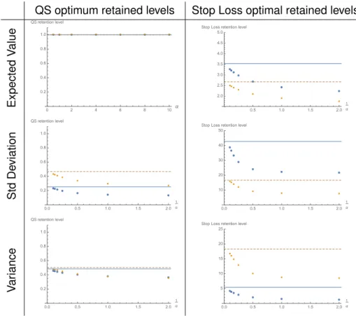
Pareto’s copula with two identical risks and the loading coefficients of Table 5.2
QS optimum retained levels Stop Loss optimal retained levels
s Expected V alue ● ● ● ● ● ● ● ■ ■ ■ ■ ■ ■ ■
0 2 4 6 8 10α
0.2 0.4 0.6 0.8 1.0 QS retention level
● ● ● ● ● ● ● ■ ■ ■ ■ ■ ■ ■
0.5 1.0 1.5 2.0
1 α 2.0 2.5 3.0 3.5 4.0 4.5 5.0 Stop Loss retention level
sp Std De viation ● ● ● ● ● ● ● ■ ■ ■ ■ ■ ■ ■
0.0 0.5 1.0 1.5 2.0
1 α 0.2 0.4 0.6 0.8 1.0 QS retention level
● ● ● ● ● ● ● ■ ■ ■ ■ ■ ■ ■
0.0 0.5 1.0 1.5 2.0
1 α 10 20 30 40 50 Stop Loss retention level
spc
V
ar
iance ●●●● ● ● ●
■ ■ ■ ■ ■ ■ ■
0.0 0.5 1.0 1.5 2.0
1 α 0.2 0.4 0.6 0.8 1.0 QS retention level
● ● ● ● ● ● ● ■ ■ ■ ■ ■ ■ ■
0.0 0.5 1.0 1.5 2.0
1 α 5 10 15 20 25 Stop Loss retention level
Figure 5.1: QS (left) and stop loss (right) optimal retained levels, computing stop loss and QS premiums separately (blue) and together (yellow), as function of the dependence
param-eter 1/α. Top: Expected value principle. Middle: Standard deviation principle. Bottom:
Variance principle. The horizontal lines correspond to the optimal retention levels in case of
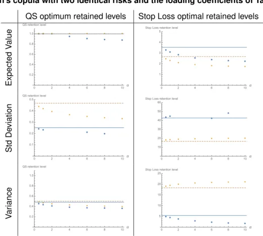
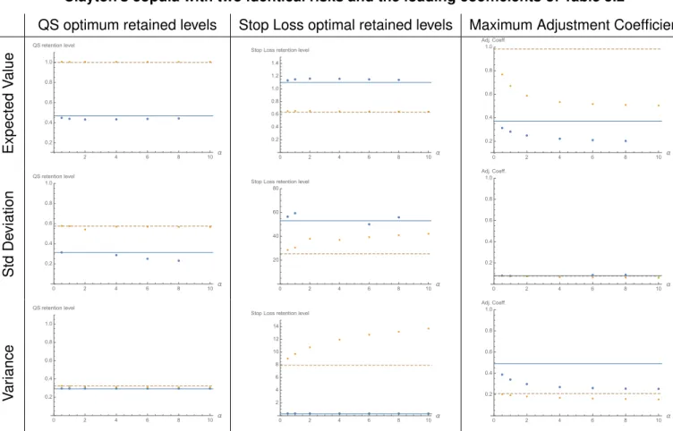
Clayton’s copula with two identical risks and the loading coefficients of Table 5.2
QS optimum retained levels Stop Loss optimal retained levels
s
Expected
V
alue
● ● ● ●
● ● ●
■ ■ ■ ■ ■ ■ ■
0 2 4 6 8 10α
0.2 0.4 0.6 0.8 1.0 QS retention level
●● ●
● ●
● ●
■ ■
■ ■
■ ■ ■
0 2 4 6 8 10α
1 2 3 4 5 Stop Loss retention level
sp
Std
De
viation ● ●
● ●
■ ■ ■
■ ■
■ ■
0 2 4 6 8 10α
0.1 0.2 0.3 0.4 0.5 QS retention level
● ● ●
●
■ ■ ■ ■ ■ ■ ■
0 2 4 6 8 10α
10 20 30 40 50 60 Stop Loss retention level
spc
V
ar
iance ● ● ●
● ● ● ●
■ ■ ■
■ ■ ■ ■
0 2 4 6 8 10α
0.2 0.4 0.6 0.8 1.0 QS retention level
● ● ● ●
● ● ●
■ ■ ■ ■
■ ■ ■
0 2 4 6 8 10α
5 10 15 20 25 Stop Loss retention level
Figure 5.2: QS (left) and stop loss (right) optimal retained levels, computing stop loss and QS premiums separately (blue) and together (yellow), as function of the dependence
pa-rameterα. Top: Expected value principle. Middle: Standard deviation principle. Bottom:
Variance principle. The horizontal lines correspond to the optimal retention levels in case of
Frank’s copula with two identical risks and the loading coefficients of Table 5.2
QS optimum retained levels Stop Loss optimal retained levels
s Expected V alue ●● ● ● ● ● ● ● ● ● ● ■■ ■ ■ ■ ■ ■ ■ ■ ■ ■
0 5 10 15 20 25 30α
0.2 0.4 0.6 0.8 1.0 QS retention level
●● ● ● ● ● ● ● ● ● ● ■■■ ■ ■ ■ ■ ■ ■ ■ ■
0 5 10 15 20 25 30α 1
2 3 4 5 Stop Loss retention level
sp Std De viation ● ● ● ● ● ● ● ■ ■ ■ ■ ■ ■ ■
0 2 4 6 8 10α
0.2 0.4 0.6 0.8 1.0 QS retention level
● ● ● ● ● ● ●
■ ■ ■ ■ ■ ■ ■
0 2 4 6 8 10α
10 20 30 40 50 Stop Loss retention level
spc
V
ar
iance ● ● ● ●
● ● ●
■ ■ ■
■ ■ ■ ■
0 2 4 6 8 10α
0.2 0.4 0.6 0.8 1.0 QS retention level
● ● ●
● ●
● ●
■ ■ ■ ■
■ ■ ■
0 2 4 6 8 10α
5 10 15 20 25 Stop Loss retention level
Figure 5.3: QS (left) and stop loss (right) optimal retained levels, computing stop loss and QS premiums separately (blue) and together (yellow), as function of the dependence
pa-rameterα. Top: Expected value principle. Middle: Standard deviation principle. Bottom:
Variance principle. The horizontal lines correspond to the optimal retention levels in case of
independence. Maximizing the expected utility with coefficient of risk aversionβ = 0.1.
The results show that dependence impacts the optimal levels of retention. Both QS and stop loss optimal retention levels vary as dependence increases. It should be noted that, although optimal stop loss retention levels change with dependence, the absolute values do not vary much. Nevertheless, the impact of dependence is evident.
For all three copulas, the optimal reinsurance using the expected value principle together for the QS and stop loss is the pure stop loss contract, regardless the dependence parameter value. This was expected, from the results in [39]. In the case of Pareto’s copula, for the expected value principle, if QS and stop loss premiums are computed separately, then the stop loss contract is still optimal, regardless the dependence parameter value. However, for Clayton’s and Frank’s copulas, as the dependence parameter increases, the QS retention level decreases.
stop loss contract, the stop loss optimal retention level decreases as dependence increases. For the Pareto’s copula, this is also true for the standard deviation and variance principles.
For all copulas and premium principles, the QS optimal retention level is below the optimal value in case of independence and decreases as dependence increases. For the Pareto’s copula, the decrease, with dependence, in the optimal QS retained level is accompanied by a decrease in the optimal stop loss retention level. This is expectable, as the Pareto’s copula has right tail behaviour. This is not the case for Calyton’s and Frank’s copulas, namely for the standard deviation and variance principles. These phenomena are related with the fact that both Clayton’s and Frank’s copulas have no right tail dependence, which is the part of the distribution covered by the stop loss contract. For these two copulas, when variance (computed on the whole ceded risk) and standard deviation (computing QS and stop loss premiums separately or together) principles are considered, the optimal solution in presence of dependence is to transfer more risk through QS than in the independent case and less risk through stop loss than in the independent case. This behaviour is not observed in the Pareto’s copula.
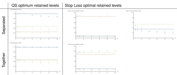
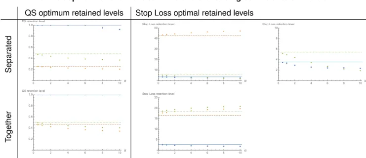
In Figures 5.4, 5.5 and 5.6, these results are presented comparing the three premium principles. When computing QS and stop loss premiums together, the standard deviation and variance premium principles produce similar results, with the standard deviation optimal retained levels below the variance ones. In this case, the optimal retained levels when using the expected value principle are significantly different from those using the standard deviation and variance principles. Indeed, the pure stop loss is the optimal treaty for the expected value principle when computing QS and stop loss premiums together. Thus, the optimal stop loss retained level in this case becomes quite lower than that of the standard deviation and variance principles, where a combination with QS is optimal. This is observable for all three copulas considered.
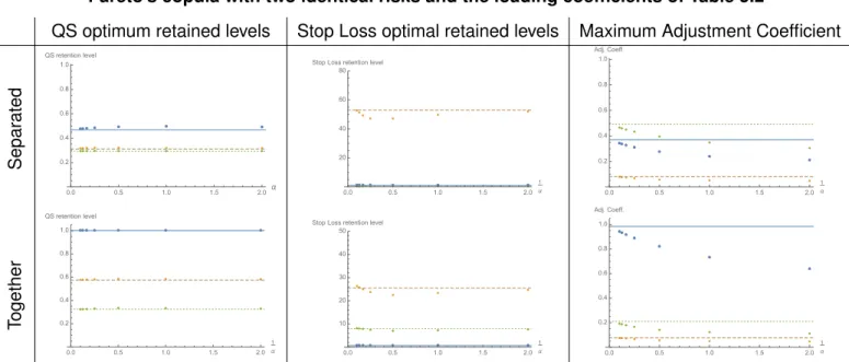
Pareto’s copula with two identical risks and the loading coefficients of Table 5.2
QS optimum retained levels Stop Loss optimal retained levels
spc Separ ated ● ● ● ● ● ● ●■■■ ■ ■ ■ ■
0.0 0.5 1.0 1.5 2.0
1 α 0.2 0.4 0.6 0.8 1.0 QS retention level
● ● ● ● ● ● ● ■ ■ ■ ■ ■ ■ ■ ◆ ◆ ◆ ◆ ◆ ◆ ◆
0.0 0.5 1.0 1.5 2.0
1 α 10 20 30 40 50 Stop Loss retention level
● ● ● ● ● ● ● ◆ ◆ ◆ ◆ ◆ ◆ ◆
0.0 0.5 1.0 1.5 2.0
1 α 2 4 6 8 10 Stop Loss retention level
spc T ogether ● ● ● ● ● ● ● ■ ■ ■ ■ ■ ■ ■ ◆ ◆ ◆ ◆ ◆ ◆ ◆
0.0 0.5 1.0 1.5 2.0
1 α 0.2 0.4 0.6 0.8 1.0 QS retention level
● ● ● ● ● ● ● ■ ■ ■ ■ ■ ■ ■ ◆ ◆ ◆ ◆ ◆ ◆ ◆
0.0 0.5 1.0 1.5 2.0
1 α 5 10 15 20 25 Stop Loss retention level
Figure 5.4: Optimal retention levels for the expected value (blue), standard deviation (yellow) and variance (green) principles, computing QS and stop loss premiums separately (top) and
together (bottom), as function of the dependence parameter1/α. Maximizing the expected
utility with coefficient of risk aversionβ = 0.1.
Clayton’s copula with two identical risks and the loading coefficients of Table 5.2
QS optimum retained levels Stop Loss optimal retained levels
spc Separ ated ● ● ● ● ● ● ● ■ ■ ■ ■ ■ ■ ◆ ◆ ◆ ◆ ◆ ◆ ◆
0 2 4 6 8 10α
0.2 0.4 0.6 0.8 1.0 QS retention level
● ● ● ● ● ● ●
■ ■ ■
■
◆ ◆ ◆ ◆ ◆ ◆ ◆
0 2 4 6 8 10α
10 20 30 40 50 Stop Loss retention level
● ● ● ● ● ● ● ◆ ◆ ◆ ◆ ◆ ◆ ◆
0 2 4 6 8 10α 2
4 6 8 10 Stop Loss retention level
spc T ogether ● ● ● ● ● ● ● ■ ■ ■ ■ ■ ■ ■ ◆ ◆ ◆ ◆ ◆ ◆ ◆
0 2 4 6 8 10α
0.2 0.4 0.6 0.8 1.0 QS retention level
● ● ● ● ● ● ●
■ ■ ■ ■
■ ■ ■
◆ ◆ ◆ ◆
◆ ◆ ◆
0 2 4 6 8 10α
5 10 15 20 25 Stop Loss retention level
Figure 5.5: Optimal retention levels for the expected value (blue), standard deviation (yellow) and variance (green) principles, computing QS and stop loss premiums separately (top) and
together (bottom), as function of the dependence parameter α. Maximizing the expected
Frank’s copula with two identical risks and the loading coefficients of Table 5.2
QS optimum retained levels Stop Loss optimal retained levels
spc Separ ated ● ● ● ● ● ● ● ■ ■ ■ ■ ■ ■ ■ ◆ ◆ ◆ ◆ ◆ ◆ ◆
0 2 4 6 8 10α
0.2 0.4 0.6 0.8 1.0 QS retention level
● ● ● ● ● ● ●
■ ■ ■ ■
■ ■ ■
◆ ◆ ◆ ◆ ◆ ◆ ◆
0 2 4 6 8 10α
10 20 30 40 50 Stop Loss retention level
● ● ● ● ● ● ● ◆ ◆ ◆ ◆ ◆ ◆ ◆
0 2 4 6 8 10α 2
4 6 8 10 Stop Loss retention level
spc T ogether ● ● ● ● ● ● ● ■ ■ ■ ■ ■ ■ ■ ◆ ◆ ◆ ◆ ◆ ◆ ◆
0 2 4 6 8 10α
0.2 0.4 0.6 0.8 1.0 QS retention level
● ● ● ● ● ● ●
■ ■ ■ ■
■ ■ ■
◆ ◆ ◆ ◆
◆ ◆ ◆
0 2 4 6 8 10α
5 10 15 20 25 Stop Loss retention level
Figure 5.6: QS (left) and stop loss (right) optimal retention levels for the expected value (blue), standard deviation (yellow) and variance (green) principles, computing QS and stop loss premiums separately (top) and together (bottom), as function of the dependence
pa-rameterα. Maximizing the expected utility with coefficient of risk aversionβ = 0.1.
The results obtained so far regard optimal retention levels maximizing the expected
util-ity. Thus, they are dependent on the choice of the coefficient of the risk aversionβ, which
was chosen to be β = 0.1. If maximizing the adjustment coefficient is considered as
op-timality criteria instead, the optimal reinsurance treaty is not dependent on this coefficient anymore. As described in Chapter 4, to obtain the optimal reinsurance treaty maximizing the adjustment coefficient, it is enough to find the optimal solution for the expected utility
problem with the coefficient of risk aversion β > 0 such that the expected utility value in
(4.14) is equal to0. In order to solve equationG(R, a1, M1, a2, M2) = 1, for(a1, M1, a2, M2)
minimizingG(R, a1, M1, a2, M2), a bisection method was applied. Amongst the root finding
numerical methods, bisection is the simplest. Although its convergence is not very fast when compared with Newton-type methods, it has the advantage of not requiring the computation
of derivatives of the functional. Also, convergence to a tolerance of10−6
was reached within
an average of10iterations, as the initial points were easily chosen close enough to the
so-lution. Situations where convergence was more difficult regard instances where converge of
the constraint global optimization algorithm to the minimum of functionalGwas slow. This
was the case of Clayton’s copula, when using the standard deviation principle computing QS and stop loss premiums separately.
coefficient for the loading coefficients in Table 5.2.
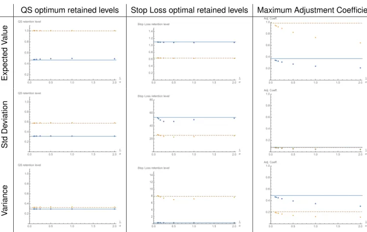
Pareto’s copula with two identical risks and the loading coefficients of Table 5.2
QS optimum retained levels Stop Loss optimal retained levels Maximum Adjustment Coefficient
s Expected V alue ● ● ● ● ● ● ● ■ ■ ■ ■ ■ ■ ■
0.0 0.5 1.0 1.5 2.0
1 α 0.2 0.4 0.6 0.8 1.0 QS retention level
● ● ● ● ● ● ● ■ ■ ■ ■ ■ ■ ■
0.0 0.5 1.0 1.5 2.0
1 α 0.2 0.4 0.6 0.8 1.0 1.2 1.4 Stop Loss retention level
● ● ● ● ● ● ● ■ ■ ■ ■ ■ ■ ■
0.0 0.5 1.0 1.5 2.0
1 α 0.2 0.4 0.6 0.8 1.0 Adj. Coeff. sp Std De viation ● ● ● ● ● ● ● ■ ■ ■ ■ ■ ■ ■
0.0 0.5 1.0 1.5 2.0
1 α 0.2 0.4 0.6 0.8 1.0 QS retention level
● ● ● ● ● ● ● ■ ■ ■ ■ ■ ■ ■
0.0 0.5 1.0 1.5 2.0
1 α 20 40 60 80 Stop Loss retention level
● ● ● ● ● ● ● ■ ■ ■ ■ ■ ■ ■
0.0 0.5 1.0 1.5 2.0
1 α 0.2 0.4 0.6 0.8 1.0 Adj. Coeff. spc V ar iance ● ● ● ● ● ● ●■■■ ■ ■ ■ ■
0.0 0.5 1.0 1.5 2.0
1 α 0.2 0.4 0.6 0.8 1.0 QS retention level
● ● ● ● ● ● ● ■ ■ ■ ■ ■ ■ ■
0.0 0.5 1.0 1.5 2.0
1 α 2 4 6 8 10 12 14 Stop Loss retention level
● ● ● ● ● ● ● ■ ■ ■ ■ ■ ■ ■
0.0 0.5 1.0 1.5 2.0
1 α 0.2 0.4 0.6 0.8 1.0 Adj. Coeff.
Figure 5.7: QS (left) and stop loss (middle) optimal retained levels, and maximum adjustment coefficient (right), computing stop loss and QS premiums separately (blue) and together
(yel-low), as function of the dependence parameter1/α.Top: Expected value principle. Middle:
Standard deviation principle.Bottom:Variance principle. The horizontal lines correspond to