MACROECONOMIC RATES OF RETURN OF PUBLIC AND PRIVATE INVESTMENT CROWDING-IN AND CROWDING-OUT EFFECTS

(1)

W O R K I N G PA P E R S E R I E S

N O 8 6

4 / F E B R U A R Y 2 0 0

8 MACROECONOMIC

RATES OF RETURN OF

PUBLIC AND PRIVATE

INVESTMENT

CROWDING

-

IN AND

CROWDING

-

OUT

EFFECTS

(2)

W O R K I N G P A P E R S E R I E S

N O 8 6 4 / F E B R U A R Y 2 0 0 8

In 2008 all ECB publications feature a motif taken from the 10 banknote.

MACROECONOMIC RATES

OF RETURN OF PUBLIC

AND PRIVATE INVESTMENT

CROWDING-IN AND

CROWDING-OUT EFFECTS

1

António Afonso

2,3

and Miguel St. Aubyn

3

This paper can be downloaded without charge from http://www.ecb.europa.eu or from the Social Science Research Network electronic library at http://ssrn.com /abstract_id=1090278.

1 We are grateful to Peter Claeys, Hubert Gabrisch, José Marín, Thomas Stratmann, and to participants at the Vereins für Socialpolitik (Bayreuth), at the Netwerk Algemene en Kwantitatieve Economie (Amesterdam), at the 63rd International Atlantic Economic Conference (Madrid), at the EcoMod (S. Paulo) conference, and to an anonymous referee for helpful comments and suggestions. The opinions expressed herein are those of the authors and do not necessarily reﬂ ect those of the ECB or the Eurosystem.

2 European Central Bank, Directorate General Economics, Kaiserstraße 29, D-60311 Frankfurt am Main, Germany; e-mail: antonio.afonso@ecb.europa.eu 3 ISEG/TULisbon – Technical University of Lisbon, Department of Economics; UECE – Research Unit on

(3)

© European Central Bank, 2008 Address

Kaiserstrasse 29

60311 Frankfurt am Main, Germany

Postal address

Postfach 16 03 19

60066 Frankfurt am Main, Germany

Telephone

+49 69 1344 0

Website

http://www.ecb.europa.eu

Fax

+49 69 1344 6000

Any reproduction, publication and reprint in the form of a different publication, whether printed or produced electronically, in whole or in part, is permitted only with the explicit written authorisation of the ECB or the author(s).

The views expressed in this paper do not necessarily reﬂ ect those of the European Central Bank.

(4)

Abstract 4

Non-technical summary 5

1 Introduction 7

2 Literature and stylised facts 8 2.1 Related literature 8 2.2 Some stylised facts 10

3 Methodology 11

3.1 VAR speciﬁ cation 11 3.2 Macroeconomic rates of return 14

4 Empirical analysis 17

4.1 Data 17

4.2 VAR estimation 18

4.3 The rates of return 20 4.4 Crowding-in and crowding-out effects 21

5 Conclusion 22

References 24

Appendix – Data sources 26

Tables and ﬁ gures 27

European Central Bank Working Paper Series 53

(5)

Abstract

Using annual data from 14 European Union countries, plus Canada, Japan and the United States, we evaluate the macroeconomic effects of public and private investment through VAR analysis. From impulse response functions, we are able to assess the extent of crowding-in or crowding-out of both components of investment. We also compute the associated macroeconomic rates of return of public and private investment for each country. The results point mostly to the existence of positive effects of public investment and private investment on output. On the other hand, the crowding-in effects of public investment on private investment vary across countries, while the crowding-in effect of private investment on public investment is more generalised.

JEL: C32, E22, E62

(6)

Non-technical summary

In this paper we address two key questions: does public investment have a significant effect on GDP, via computing macroeconomic rates of return, and does public investment induce more private investment. From a theoretical perspective, a rise in public investment can have two effects on private investment. First, the increase of public investment needs to be financed, which may imply more taxes or impose a higher demand for funds from the government in the capital markets, therefore causing interest rates to rise. This would reduce the amount of savings available for private investors and decrease the expected rate of return of private capital, leading to a crowding-out effect on private investment. Second, public investment can create additional favourable conditions for private investment, for instance, by providing or promoting relevant infrastructure such as roads, highways, sewage systems, harbours or airports. The existence of infrastructure facilities may increase the productivity of private investment, which can then take advantage of better overall infrastructures and potentially improved business conditions. This would result in having a crowding-in effect on private investment.

Our work contains some innovative features worth mentioning. First, and for the first time in the literature, public partial and total investment rates of return derived from a VAR procedure are systematically computed and compared across countries and periods of time. Secondly, we extend our analysis and methodology towards the consideration of innovations in private investment, and therefore we are also able to compute private investment rates of return. This allows us to analyse not only the more studied question of private investment being crowded in or out by public investment, but also the effects of private investment on public capital formation decisions.

In our paper, by estimating VARs for 14 European Union countries, plus Canada, Japan and the United States, we estimated that, between 1960 and 2005:

(7)

- on the other hand, expansionary effects and crowding-in prevailed in eight cases (Austria, Germany, Denmark, Finland, Greece, Portugal, Spain and Sweden).

These effects correspond to point estimates and care should be taken in their interpretation, as 95 percent confidence bands concerning public investment effects on output always include the zero value.

When it is possible to compute it, the partial rate of return of public investment is mostly positive, with the exceptions of Finland, Italy and Sweden. Taking into account the induced effect on private investment, the total rate of return associated with public investment is generally lower, with the exception of France, and negative for the cases of Austria, Finland, Greece, Portugal and Sweden, countries where the increase in GDP was not sufficiently high to compensate for the total investment effort.

(8)

1. Introduction

In this paper we address two key questions: does public investment have a significant effect on GDP, via computing macroeconomic rates of return, and does public investment induce more private investment. In other words, we ask if crowding-in prevails or else, if the main result is crowding-out. From a theoretical perspective, a rise in public investment can have two effects on private investment. First, the increase of public investment needs to be financed, which may imply more taxes or impose a higher demand for funds from the government in the capital markets, therefore causing interest rates to rise. This would reduce the amount of savings available for private investors and decrease the expected rate of return of private capital, leading to a crowding-out effect on private investment. Second, public investment can create additional favourable conditions for private investment, for instance, by providing or promoting relevant infrastructure such as roads, highways, sewage systems, harbours or airports. The existence of infrastructure facilities may increase the productivity of private investment, which can then take advantage of better overall infrastructures and potentially improved business conditions. This would result in having a crowding-in effect on private investment.

(9)

functions to assess the extent of crowding-in or crowding-out of both components of investment.

Our work contains some innovative features worth mentioning. First, and for the first time in the literature, public partial and total investment rates of return derived from a VAR procedure are systematically computed and compared across countries and periods of time. Secondly, we extend our analysis and methodology towards the consideration of innovations in private investment, and therefore we are also able to compute private investment rates of return. This allows us to analyse not only the more studied question of private investment being crowded in or out by public investment, but also the effects of private investment on public capital formation decisions.

The paper is organised as follows. In Section Two we briefly review some of the literature and previous results. Section Three outlines the methodological approach used in the paper both regarding the VAR specification and the analytical framework to compute the macroeconomic rates of return. In Section four we present and discuss our results. Section Five summarise the paper’s main findings.

2. Literature and stylised facts

2.1. Related literature

(10)

called for the exclusion of public investment from the budget deficit threshold established under the Maastricht Treaty. Moreover, the significance of public investment has been further illustrated by the idea of the Golden Rule, suggesting that such spending should only be financed by issuing government debt, and also by the imposition of formal rules that budget deficits cannot exceed public investment.1

Since Aschauer’s (1989a, 1989b) initial contributions regarding the derivation of the elasticity of output with respect to public capital stock, there has been considerable interest in measuring the effects of public investment on aggregate economic activity, as well as in assessing whether public investment crowds in or crowds out private investment. The results of Aschauer (1989b) indicated that for the US, public investment had an overall crowding-in effect on private investment, and that public and private capital could be seen as complementary.2 Therefore, the related relevant economic policy question seems to be whether or not public government investment is productive and does contribute positively to growth, either directly or indirectly via private investment decisions.

Some related studies have addressed the effects of public investment on GDP, and the crowding-in hypothesis in the context of VAR analysis. For instance, Voss (2002) estimates a VAR model with GDP, public investment, private investment, the real interest rate, and price deflators of private and public investment, for the US and Canada, for the period 1947-1996. According to the reported results, innovations to public investment crowd out private investment. Mittnik and Neumann (2001)

1

Musgrave (1939) discussed the appropriateness of financing via government debt, the so-called self-liquidating investments, which he critically considered to be limited.

2

(11)

estimate a VAR with GDP, private investment, public investment and public consumption for six industrialised economies. Their results indicate that public investment tends to exert positive effects on GDP, and that there is no evidence of dominant crowding-out effects.

Argimón, González-Páramo and Roldán (1997) present results that support the existence of a crowding-in effect of private investment by public investment, through the positive impact of infrastructure on private investment productivity, for a panel of 14 OECD countries. Additionally, Perotti (2004) and Kamps (2004) assess the output and labour market effects of government investment in a VAR context.

2.2. Some stylised facts

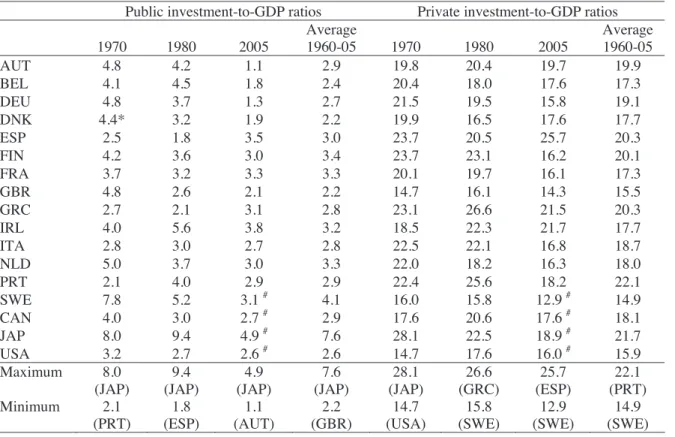
The share of both public and private investment in GDP varies across our country sample and also throughout the time sample dimension. These developments are summarised in Table 1.

(12)

investment ratios were already on a downward path.3 Additionally, it is also possible to observe a decline from quite above-average sample levels in the investment ratio for the case of Japan, and a rather stable ratio for the US.

In terms of private investment ratios, some heterogeneity also prevails in our country sample. For instance, in 1970, private investment-to-GDP ratios ranged from around 15 per cent in such countries as the UK, the US and Sweden, to around 24 per cent in the cases of Finland, Spain; the ratio even went as high as 28 per cent in the case of Japan. In more recent years, the private investment-to-GDP in Spain was above average, while some upward trends were visible from the second half of the 1990s onwards in countries such as France, Ireland, Italy, Spain and the US.

3. Methodology

3.1. VAR specification

We estimate a small five-variable VAR model for each country throughout the period 1960-2005. The variables in the VAR are the logarithmic growth rates of real public investment, Ipub, real private investment, Ipriv, real output, Y, real taxes, Tax, and real interest rates, R. The inclusion of output, private investment and public investment is crucial in what concerns the computation of macroeconomic rates of return, as explained later. Taxes and real interest rates are included as they may have important linkages with the above mentioned key variables.

The VAR model in standard form can be written as

1

p

t i t i t

i

X c

¦

A X H . (1)

3

(13)

where Xt denotes the (5 1)u vector of the five endogenous variables given

byX_t { '

>

logIpub_t 'logIpriv_t 'logY_t 'logTax_t 'R_t

@

', c is a (5 1)u vector of intercept terms, A is the matrix of autoregressive coefficients of order (5 5)u , and the vector of random disturbancesH_t { ¬ªH_tIpub H_tIpriv H_tY H_tTax H_tRº_¼' contains the reduced form OLS residuals. The lag length of the endogeneous variables, p, will be determined by the usual information criteria.

By imposing of a set of restrictions, it is possible to identify orthogonal shocks, K, for each of the variables in (1), and to compute these orthogonal innovations via the random disturbances:

t B t

K H . (2)

The estimation of (1) allows Cov(H) to be determined. Therefore, with the orthogonal restrictions and by means of an adequate normalisation we have Cov(K)=I, where

(5 5)

I u identity matrix, and we can write

( )_t ( _t) ( ) '_t

CovK Cov BH BCov H B , (3)

( ) '_t

I BCov H B . (4)

(14)

covariances.4 For the complete identification of the model we need ten more restrictions. The use of a Choleski decomposition of the matrix of covariances of the residuals, which requires all elements above the principal diagonal to be zero, provides the necessary additional ten restrictions, and the system is then exactly identified.

We can then impose a lower triangular structure to B-1,

11

21 22 1

31 32 33

41 42 43 44

51 52 53 54 55

0 0 0 0 0 0 0 0 0 0

d

d d

B D d d d

d d d d

d d d d d

ª º

« »

¬ ¼

, (5)

which makes possible to write the residualsH_tas a function of the orthogonal shocks in each of the variables:

t D t

H K . (6)

Our VAR is ordered from the most exogenous variable to the least exogenous one, with public investment ordered first. As a result, a shock in public investment may have an instantaneous effect on all the other variables. However, public investment does not respond contemporaneously to any structural disturbances to the remaining variables due, for instance, to lags in government decision-making. In other words,

4

(15)

private investment, GDP, taxes and the real interest rate affect public investment sequences with a one-period lag. For instance, a shock in private investment, the second variable, does not have an instantaneous impact on public investment – only on output, taxes and the real interest rate.

Moreover, this ordering implies that private investment responds to public investment in a contemporaneous fashion, but not to shocks to the other variables. Indeed, one can recall that governments typically announce their spending and investment plans in advance, in the context of their budgetary planning. Therefore, economic agents can use such information in making their investment decisions. Additionally, private investment affects GDP contemporaneously. The real interest rate is the least exogenous variable, and it is assumed that its shocks do not affect the other variables simultaneously. Moreover, it does react contemporaneously to shocks to the remaining variables in the model.

3.2. Macroeconomic rates of return

Based on impulse response functions, we compute four different rates of return: -r1, the partial rate of return of public investment;

- r2, the rate of return of total investment (originated by an impulse to public

investment);

-r3, the partial rate of return of private investment;

- r4, the rate of return of total investment (originated by an impulse to private

(16)

The partial rate of return of public investment is computed as suggested by Pereira (2000). Following an orthogonal impulse to public investment, we can compute the long-run accumulated elasticity of Y with respect to public investment, Ipub, derived from the accumulated impulse response functions of the VAR, as

log log

Ipub

Y Ipub

H '

' . (7)

The above mentioned long-run elasticity is the ratio between the accumulated change in the growth rate of output and the accumulated change in the growth rate of public investment, which will be obtained from the estimation of the country-specific VAR models.

The long-term marginal productivity of public investment is given by

Ipub

Y Y

MPIpub

Ipub H Ipub

' {

' . (8)

Then r1, the partial-cost dynamic feedback rate of return of public investment, is

obtained as the solution for:

20 1

(1r) MPIpub. (9)

(17)

crowd in or crowd out private investment respectively. Suppose, for example, that more public capital induces more private investment. The total investment that caused the detected product increase exceeds the public effort, and if one only considers the latter, the rate of return is overstated.

Since private investment also changes, the long-term accumulated elasticity of Y with respect to Ipriv can also be derived from accumulated impulse response functions of the VAR in a similar fashion:

log log

Ipriv

Y Ipriv

H '

' , (10)

and now the long-term marginal productivity of private investment is given by

Ipriv

Y Y

MPIpriv

Ipriv H Ipriv

' {

' . (11)

Therefore, computing the marginal productivity of total investment, MPTI, implies taking into account both the long-term marginal productivity of public and private investment, as follows:

1 1

1

Y MPTI

Ipub Ipriv MPIpub MPIpriv

'

(18)

Following Pina and St. Aubyn (2006), we compute a rate of return of total investment. The rate of return of total investment (originated by an impulse to public investment),

r2, is obtained as the solution for:

MPTI r

20

2)

1

( . (13)

In our described benchmark framework we use 20 years to compute both the partial and the total rates of return. In other words, we assume an average life of 20 years for a capital good. For instance, while the average life of a personal computer could be three or four years, the life expectancy of a bridge is certainly to be measured in decades.

The partial rate of return of private investment, r3,is computed in a way analogous to

r1. Using the accumulated impulse responses of the VAR following an impulse on

private investment, the long-run output elasticity is obtained, and then a marginal productivity and a rate of return can be calculated. As public investment may also respond positively or negatively to private efforts, a rate of return of total investment,

r4, is also estimated.

4. Empirical analysis

4.1. Data

(19)

2005), Sweden (1971–2004) and the UK (1970–2005), plus Canada (1964–2004), Japan (1972–2004), and the United States (1961–2004). In order to estimate our VAR for each country, we use information for the following series: GDP at current market prices; price deflator of GDP; general government gross fixed capital formation at current prices, used as public investment; gross fixed capital formation of the private sector at current prices, used as private investment; direct taxes, indirect taxes and social contributions, aggregated into taxes; the nominal long-term interest rate and the consumer price index..

GDP, taxes and investment variables are transformed into real values using the price deflator of GDP and the price deflator of the gross fixed capital formation of the total economy.5 A real ex-post interest rate is computed using the consumer price index inflation rate. All data are taken from the European Commission Ameco database.6

4.2. VAR estimation

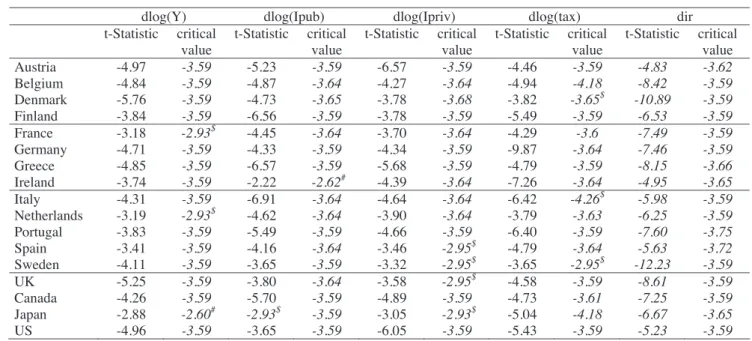
In the estimation of each country’s VAR, its GDP, public investment, private investment, taxes and the interest rate are used in real terms. All variables enter the VAR as logarithmic growth rates, except the interest rate, where first differences of original values were taken. Moreover, the unit root analysis that we undertook showed that these first differenced variables are mostly stationary, I (0) time series. Table 2 shows unit root test stastistics.

5

Due to the lack of information on a price deflator for private investment, we use the same deflator to compute both public and private investment variables.

6

(20)

Note that we chose not to estimate a “levels VAR” or to infer possible co-integration vectors. In fact, there is no theoretical reason to expect a long-run relationship between public investment, private investment, taxes, the real interest rate and GDP, or between any two of these three variables, and to force this relationship could introduce an unwanted structure into our empirical endeavour.

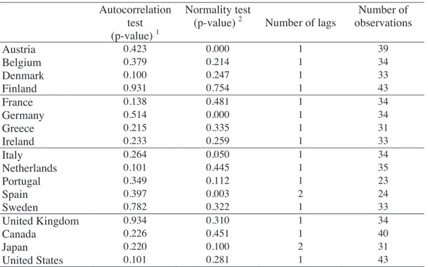
The chosen VAR order used in the estimation of each model was selected with the Akaike and the Schwarz information criteria. Those tests led us to choose a more parsimonious model with only one lag for most of the countries, which helped avoid the use of too many degrees of freedom. With such specifications we usually could not reject the null hypothesis of no serial residual correlation. In addition, we did not reject the null hypothesis of normality of the VAR residuals in most cases. The diagnostic tests regarding residual autocorrelation and normality are also reported in Table 3.

Additionally, for the case of Germany we included a dummy variable that takes the value of one in 1991 and zero otherwise in order to capture the break in the series related to German reunification. This variable is highly statistically significant in all equations. Moreover, for all cases we chose to privilege the absence of autocorrelation of the residuals, even in the eventuality of the residuals being non-normal.7 As can be seen from Table 3, all p-values exceed ten per cent. Therefore, even at a significance level of 10 per cent, the null hypothesis of no residual autocorrelation cannot be rejected for all countries.

7

(21)

4.3. The rates of return

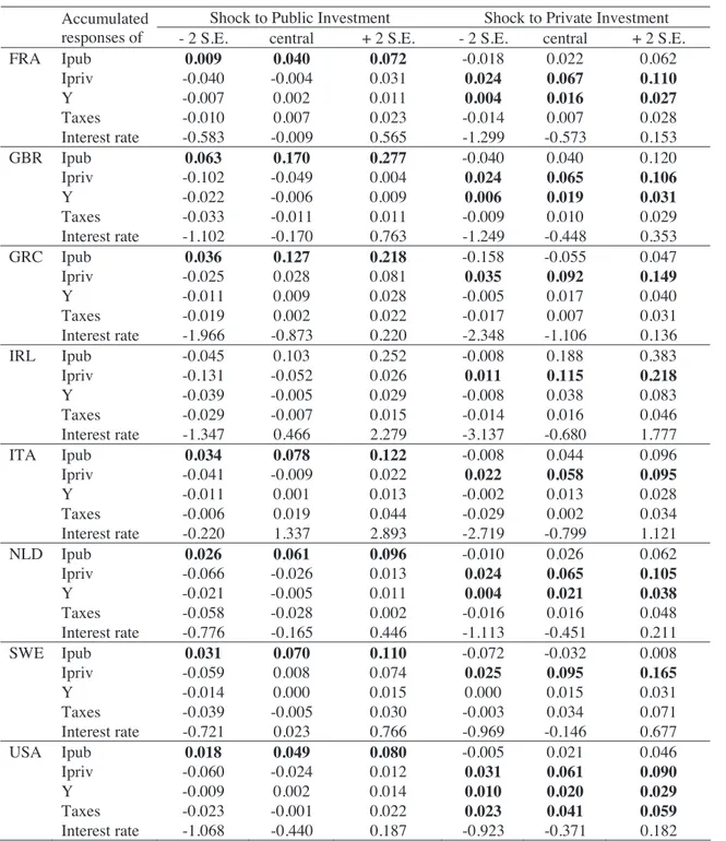
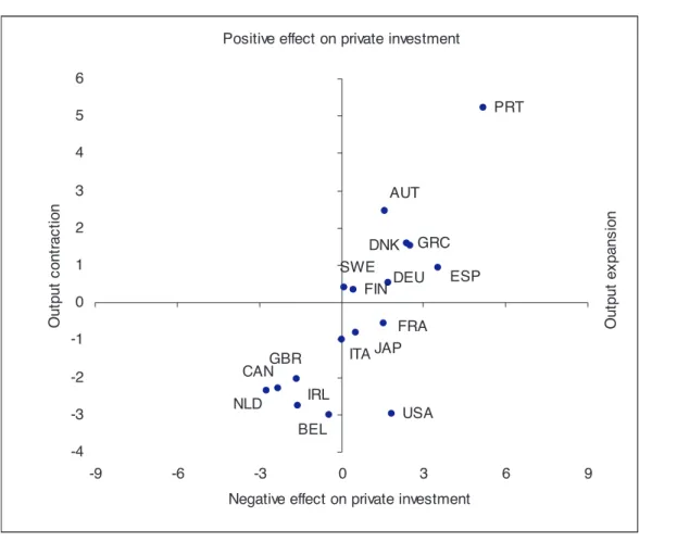
Table 4 contains information on accumulated responses of all VAR variables to public and private investment innovations (the impulse response functions are plotted in the Annex). A 95 percent (two standard deviations) confidence band around estimates is also included. Figures in bold correspond to cases where those confidence bands include positive or negative values only. Note that impulses to public investment are never statistically significant at 95 percent level in what concerns effects on other variables. On the other hand, impulses to private investment have in most cases a positive and significant impact on output, and in some instances on taxes.

Table 5 reports the computed output elasticity and the rates of return of public and private investment for each country for the respective period of available data. Overall, one can observe that the output elasticity of private investment is always positive and higher than the output elasticity of public investment.

In those cases where rates of return can be calculated or, in other words, whenever the marginal productivity is positive, the partial rate of return of public investment is mostly positive, with the exceptions of Finland, Italy and Sweden. Taking into account the induced effect on private investment, the total rate of return associated with public investment is generally lower, with the exception of France, and even negative for the cases of Austria, Finland, Greece, Portugal and Sweden.

(22)

on public investment. The partial rates of return of private investment are mostly positive, with the exception of Belgium, Denmark and Greece, where the rate is moderately negative. The total rate of return of private investment is mostly somewhat below the partial rate of return, albeit slightly higher in the cases of Italy, Greece and Sweden.

4.4. Crowding-in and crowding-out effects

On the basis of the values of the partial marginal productivity of public investment, it is possible to determine the impact of public investment on output. That information, taken from Table 5, is displayed on the horizontal axis of Figure 1. Additionally, on the vertical axis we plot the marginal effects of public investment on private investment, which allows us to assess the possible existence of crowding-in or crowding-out effects of public investment on private investment. Such effects can be easily derived from

Ipub

Ipriv

Ipriv Ipriv

Ipub Ipub

H H

'

' . (14)

(23)

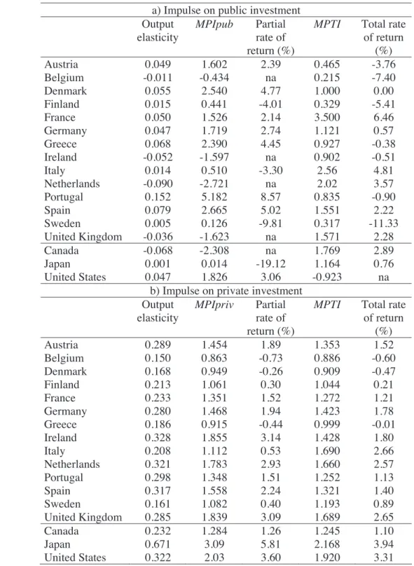
Figure 2 shows the values of the marginal productivity of private investment and the marginal effects of private investment on public investment. This chart is useful in visualising both the effect of private investment on output and the existing crowding-in or crowdcrowding-ing-out effects of private crowding-investment on public crowding-investment.

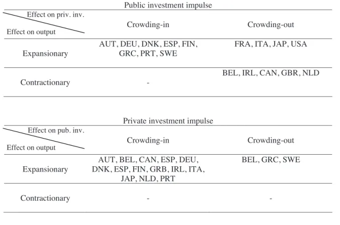
Figure 2 also reveals that private investment has a crowding-in effect on public investment for most of the countries in the sample, while it crowds out public investment in the cases of Belgium, Greece and Sweden. In addition, private investment has an expansionary effect on output for all countries in the sample. The effects of both public and private investment impulses for all countries are summarised in Figure 3.

Finally, we also performed a sensitivity analysis by using only ten years for both public and private investment, and also by assuming differentiated horizons, with twenty and ten years respectively for public and for private investment. The results, not reported in the paper, provided similar overall conclusions.

5. Conclusion

(24)

- public investment had a contractionary effect on output in five cases (Belgium, Ireland, Canada, the United Kingdom and the Netherlands) with positive public investment impulses leading to a decline in private investment (crowding-out);

- on the other hand, expansionary effects and crowding-in prevailed in eight cases (Austria, Germany, Denmark, Finland, Greece, Portugal, Spain and Sweden).8

These effects correspond to point estimates and care should be taken in their interpretation, as 95 percent confidence bands concerning public investment effects on output always include the zero value.

When it is possible to compute it, the partial rate of return of public investment is mostly positive, with the exceptions of Finland, Italy, Japan and Sweden. Taking into account the induced effect on private investment, the total rate of return associated with public investment is generally lower, with the exception of France, and negative for the cases of Austria, Finland, Greece, Portugal and Sweden, countries where the increase in GDP was not sufficiently high to compensate for the total investment effort.

Private investment impulses, by contrast, were always expansionary in GDP terms and effects were usually significant in statistical terms. Public investment responded positively to private investment in all but three countries (Belgium, Greece and Sweden). The highest estimated return was in Japan (5.81 percent, partial), and there

8

(25)

were very few cases of slightly negative private investment rates of return, either partial or total – Belgium, Denmark and Greece.

References

Argimón, I., González-Páramo, J. and Roldán, J. (1997). Evidence of public spending crowding-out from a panel of OECD countries. Applied Economics, 29 (8), 1001-1010.

Aschauer, D. (1989a). Is Public Expenditure Productive? Journal of Monetary Economics 23 (2), 177-200.

Aschauer, D. (1989b). Does public capital crowd out private capital? Journal of Monetary Economics 24 (2), 171-188.

Kamps, C. (2004). The dynamic effects of public capital: VAR evidence for 22 OECD countries, Kiel Institute, Working Paper 1224.

Lütkepohl, H. (2005). New introduction to multiple time series analysis. Berlin, Springer.

Mittnik, S., Neumann, T. (2001). Dynamic effects of public investment: Vector autoregression evidence from six industrialized countries. Empirical Economics 26, 429-446.

Musgrave, R. (1939). The Nature of Budgetary Balance and the Case for the Capital Budget.American Economic Review 29 (2), 260-271.

Pereira, A. (2000). Is All Public Capital Created Equal? Review of Economics and Statistics 82 (3), 513-518.

(26)

Pina, A. and St. Aubyn, M. (2005). Comparing macroeconomic returns on human and public capital: An empirical analysis of the Portuguese case (1960–2001). Journal of Policy Modelling 27, 585-598.

Pina, A. and St. Aubyn, M. (2006). How should we measure the return on public investment in a VAR? Economics Bulletin 8(5), 1-4

Voss, G. (2002). Public and private investment in the United States and Canada.

Economic Modelling 19, 641-664.

Zou, Y. (2006). Empirical studies on the relationship between public and private

(27)

Appendix – Data sources

Original series Ameco codes *

Gross Domestic Product at current market prices, thousands national currency.

1.0.0.0.UVGD

Price deflator of Gross Domestic Product, national currency, 1995 = 100. 3.1.0.0.PVGD

Gross fixed capital formation at current prices; general government, national currency.

1.0.0.0.UIGG

Gross fixed capital formation at current prices; private sector, national currency.

1.0.0.0.UIGP

Price deflator gross fixed capital formation; total economy, national currency; 1995 = 100.

3.1.0.0.PIGT

Nominal long-term interest rates - % .1.1.0.0.ILN National consumer price index - 1995 = 100 .3.0.0.0.ZCPIN Current taxes on income and wealth (direct taxes); general government -

National currency, current prices .1.0.0.0.UTYGF Taxes linked to imports and production (indirect taxes); general

government - National currency, current prices

.1.0.0.0.UTVGF

Social contributions received; general government - National currency, current prices

.1.0.0.0.UTSGF

(28)

Tables and figures

Table 1 – Public and private investment -to-GDP ratios

Public investment-to-GDP ratios Private investment-to-GDP ratios

1970 1980 2005

Average

1960-05 1970 1980 2005

Average 1960-05

AUT 4.8 4.2 1.1 2.9 19.8 20.4 19.7 19.9

BEL 4.1 4.5 1.8 2.4 20.4 18.0 17.6 17.3

DEU 4.8 3.7 1.3 2.7 21.5 19.5 15.8 19.1

DNK 4.4* 3.2 1.9 2.2 19.9 16.5 17.6 17.7

ESP 2.5 1.8 3.5 3.0 23.7 20.5 25.7 20.3

FIN 4.2 3.6 3.0 3.4 23.7 23.1 16.2 20.1

FRA 3.7 3.2 3.3 3.3 20.1 19.7 16.1 17.3

GBR 4.8 2.6 2.1 2.2 14.7 16.1 14.3 15.5

GRC 2.7 2.1 3.1 2.8 23.1 26.6 21.5 20.3

IRL 4.0 5.6 3.8 3.2 18.5 22.3 21.7 17.7

ITA 2.8 3.0 2.7 2.8 22.5 22.1 16.8 18.7

NLD 5.0 3.7 3.0 3.3 22.0 18.2 16.3 18.0

PRT 2.1 4.0 2.9 2.9 22.4 25.6 18.2 22.1

SWE 7.8 5.2 3.1 # 4.1 16.0 15.8 12.9 # 14.9

CAN 4.0 3.0 2.7 # 2.9 17.6 20.6 17.6 # 18.1

JAP 8.0 9.4 4.9 # 7.6 28.1 22.5 18.9 # 21.7

USA 3.2 2.7 2.6 # 2.6 14.7 17.6 16.0 # 15.9

Maximum 8.0 (JAP)

9.4 (JAP)

4.9 (JAP)

7.6 (JAP)

28.1 (JAP)

26.6 (GRC)

25.7 (ESP)

22.1 (PRT) Minimum 2.1

(PRT)

1.8 (ESP)

1.1 (AUT)

2.2 (GBR)

14.7 (USA)

15.8 (SWE)

12.9 (SWE)

14.9 (SWE)

(29)

Table 2 – Unit root tests, variables in first differences: Augmented Dickey-Fuller test statistics

dlog(Y) dlog(Ipub) dlog(Ipriv) dlog(tax) dir

t-Statistic critical value

t-Statistic critical value Austria -4.97 -3.59 -5.23 -3.59 -6.57 -3.59 -4.46 -3.59 -4.83 -3.62

Belgium -4.84 -3.59 -4.87 -3.64 -4.27 -3.64 -4.94 -4.18 -8.42 -3.59

Denmark -5.76 -3.59 -4.73 -3.65 -3.78 -3.68 -3.82 -3.65$ -10.89 -3.59

Finland -3.84 -3.59 -6.56 -3.59 -3.78 -3.59 -5.49 -3.59 -6.53 -3.59

France -3.18 -2.93$ _-4.45 _-3.64 _-3.70 _-3.64 _-4.29 _{-3.6 -7.49 -3.59} Germany -4.71 -3.59 -4.33 -3.59 -4.34 -3.59 -9.87 -3.64 -7.46 -3.59

Greece -4.85 -3.59 -6.57 -3.59 -5.68 -3.59 -4.79 -3.59 -8.15 -3.66

Ireland -3.74 -3.59 -2.22 -2.62# _-4.39 _-3.64 _-7.26 _{-3.64 -4.95 -3.65} Italy -4.31 -3.59 -6.91 -3.64 -4.64 -3.64 -6.42 -4.26$_{-5.98 -3.59} Netherlands -3.19 -2.93$ -4.62 -3.64 -3.90 -3.64 -3.79 -3.63 -6.25 -3.59

Portugal -3.83 -3.59 -5.49 -3.59 -4.66 -3.59 -6.40 -3.59 -7.60 -3.75

Spain -3.41 -3.59 -4.16 -3.64 -3.46 -2.95$ -4.79 -3.64 -5.63 -3.72

Sweden -4.11 -3.59 -3.65 -3.59 -3.32 -2.95$ -3.65 -2.95$ -12.23 -3.59

UK -5.25 -3.59 -3.80 -3.64 -3.58 -2.95$ -4.58 -3.59 -8.61 -3.59

Canada -4.26 -3.59 -5.70 -3.59 -4.89 -3.59 -4.73 -3.61 -7.25 -3.59

Japan -2.88 -2.60# -2.93$ -3.59 -3.05 -2.93$ -5.04 -4.18 -6.67 -3.65

US -4.96 -3.59 -3.65 -3.59 -6.05 -3.59 -5.43 -3.59 -5.23 -3.59

(30)

Table 3 – Diagnostic tests, dynamic feedbacks VAR

Autocorrelation test

(p-value)1

Normality test

(p-value)2 Number of lags

Number of observations

Austria 0.423 0.000 1 39

Belgium 0.379 0.214 1 34

Denmark 0.100 0.247 1 33

Finland 0.931 0.754 1 43

France 0.138 0.481 1 34

Germany 0.514 0.000 1 34

Greece 0.215 0.335 1 31

Ireland 0.233 0.259 1 33

Italy 0.264 0.050 1 34

Netherlands 0.101 0.445 1 35

Portugal 0.349 0.112 1 23

Spain 0.397 0.003 2 24

Sweden 0.782 0.322 1 33

United Kingdom 0.934 0.310 1 34

Canada 0.226 0.451 1 40

Japan 0.220 0.100 2 31

United States 0.101 0.281 1 43

Notes: We considered the maximum VAR order to be three. For Germany we included a dummy variable that takes the value one in 1991 and zero otherwise. For Finland and Sweden, a similar dummy variable for 1992 was not statistically significant.

1 – Multivariate residual serial correlation LM test. For the null hypothesis of no serial autocorrelation (of order 1) the test statistic as an asymptotic chi-square distribution with k2

(31)

Table 4 – Accumulated responses to shocks in public and in private investment

Shock to Public Investment Shock to Private Investment Accumulated

responses of - 2 S.E. central + 2 S.E. - 2 S.E. central + 2 S.E.

DEU Ipub 0.027 0.048 0.069 -0.010 0.015 0.039

Ipriv -0.028 0.004 0.036 0.030 0.066 0.102

Y -0.007 0.002 0.011 0.008 0.019 0.029

Taxes -0.222 -0.080 0.063 -0.166 0.009 0.185

Interest rate -0.281 0.026 0.334 -0.463 -0.084 0.295

PRT Ipub -0.009 0.149 0.308 -0.075 0.085 0.244

Ipriv -0.059 0.103 0.266 -0.017 0.146 0.309

Y -0.030 0.023 0.075 -0.010 0.044 0.097

Taxes -0.031 0.027 0.086 -0.010 0.049 0.109

Interest rate -2.710 -0.839 1.031 -3.534 -1.640 0.253

BEL Ipub 0.051 0.109 0.166 -0.073 -0.016 0.041

Ipriv -0.101 -0.046 0.009 0.035 0.089 0.143

Y -0.013 -0.001 0.010 0.001 0.013 0.025

Taxes -0.027 -0.005 0.018 -0.026 -0.001 0.024

Interest rate -0.818 0.003 0.823 -1.434 -0.557 0.319

FIN Ipub 0.041 0.072 0.103 -0.022 0.009 0.040

Ipriv -0.054 0.004 0.063 0.036 0.097 0.157

Y -0.018 0.001 0.020 0.001 0.021 0.041

Taxes -0.019 0.006 0.031 -0.002 0.025 0.051

Interest rate -0.642 0.471 1.584 -1.232 -0.017 1.198

DNK Ipub 0.059 0.132 0.206 -0.029 0.042 0.114

Ipriv -0.049 0.025 0.099 0.048 0.120 0.193

Y -0.005 0.007 0.020 0.008 0.020 0.032

Taxes -0.005 0.018 0.041 0.009 0.032 0.056

Interest rate -0.933 -0.301 0.330 -0.907 -0.244 0.420

AUT Ipub 0.043 0.098 0.152 -0.023 0.029 0.082

Ipriv -0.024 0.005 0.033 0.030 0.057 0.083

Y -0.010 0.004 0.018 0.002 0.016 0.030

Taxes -0.022 -0.001 0.020 0.003 0.024 0.045

Interest rate -0.385 0.018 0.421 -0.850 -0.443 -0.036

CAN Ipub 0.032 0.058 0.084 -0.011 0.012 0.034

Ipriv -0.057 -0.022 0.014 0.028 0.061 0.093

Y -0.018 -0.004 0.011 0.000 0.014 0.028

Taxes -0.027 -0.006 0.014 0.006 0.026 0.045

Interest rate -0.507 0.099 0.705 -1.180 -0.592 -0.003

JAP Ipub -0.035 0.088 0.210 -0.089 0.073 0.235

Ipriv -0.082 -0.030 0.022 -0.018 0.060 0.138

Y -0.039 0.000 0.040 -0.012 0.040 0.093

Taxes -0.083 -0.005 0.073 -0.018 0.085 0.188

Interest rate -1.675 0.480 2.635 -1.713 1.104 3.921

ESP Ipub -0.048 0.040 0.127 -0.066 0.087 0.240

Ipriv -0.040 0.004 0.048 -0.008 0.071 0.150

Y -0.010 0.003 0.016 -0.001 0.022 0.046

Taxes -0.031 -0.002 0.026 -0.008 0.041 0.091

Interest rate -0.614 0.218 1.049 -1.493 -0.131 1.231

(32)

Table 4 – Accumulated responses to shocks in public and in private investment (cont.)

Shock to Public Investment Shock to Private Investment Accumulated

responses of - 2 S.E. central + 2 S.E. - 2 S.E. central + 2 S.E.

FRA Ipub 0.009 0.040 0.072 -0.018 0.022 0.062

Ipriv -0.040 -0.004 0.031 0.024 0.067 0.110

Y -0.007 0.002 0.011 0.004 0.016 0.027

Taxes -0.010 0.007 0.023 -0.014 0.007 0.028

Interest rate -0.583 -0.009 0.565 -1.299 -0.573 0.153

GBR Ipub 0.063 0.170 0.277 -0.040 0.040 0.120

Ipriv -0.102 -0.049 0.004 0.024 0.065 0.106

Y -0.022 -0.006 0.009 0.006 0.019 0.031

Taxes -0.033 -0.011 0.011 -0.009 0.010 0.029

Interest rate -1.102 -0.170 0.763 -1.249 -0.448 0.353

GRC Ipub 0.036 0.127 0.218 -0.158 -0.055 0.047

Ipriv -0.025 0.028 0.081 0.035 0.092 0.149

Y -0.011 0.009 0.028 -0.005 0.017 0.040

Taxes -0.019 0.002 0.022 -0.017 0.007 0.031

Interest rate -1.966 -0.873 0.220 -2.348 -1.106 0.136

IRL Ipub -0.045 0.103 0.252 -0.008 0.188 0.383

Ipriv -0.131 -0.052 0.026 0.011 0.115 0.218

Y -0.039 -0.005 0.029 -0.008 0.038 0.083

Taxes -0.029 -0.007 0.015 -0.014 0.016 0.046

Interest rate -1.347 0.466 2.279 -3.137 -0.680 1.777

ITA Ipub 0.034 0.078 0.122 -0.008 0.044 0.096

Ipriv -0.041 -0.009 0.022 0.022 0.058 0.095

Y -0.011 0.001 0.013 -0.002 0.013 0.028

Taxes -0.006 0.019 0.044 -0.029 0.002 0.034

Interest rate -0.220 1.337 2.893 -2.719 -0.799 1.121

NLD Ipub 0.026 0.061 0.096 -0.010 0.026 0.062

Ipriv -0.066 -0.026 0.013 0.024 0.065 0.105

Y -0.021 -0.005 0.011 0.004 0.021 0.038

Taxes -0.058 -0.028 0.002 -0.016 0.016 0.048

Interest rate -0.776 -0.165 0.446 -1.113 -0.451 0.211

SWE Ipub 0.031 0.070 0.110 -0.072 -0.032 0.008

Ipriv -0.059 0.008 0.074 0.025 0.095 0.165

Y -0.014 0.000 0.015 0.000 0.015 0.031

Taxes -0.039 -0.005 0.030 -0.003 0.034 0.071

Interest rate -0.721 0.023 0.766 -0.969 -0.146 0.677

USA Ipub 0.018 0.049 0.080 -0.005 0.021 0.046

Ipriv -0.060 -0.024 0.012 0.031 0.061 0.090

Y -0.009 0.002 0.014 0.010 0.020 0.029

Taxes -0.023 -0.001 0.022 0.023 0.041 0.059

Interest rate -1.068 -0.440 0.187 -0.923 -0.371 0.182

(33)

Table 5 – Long-run elasticities, marginal productivity and rates of return (full period)

a) Impulse on public investment Output

elasticity

MPIpub Partial rate of return (%)

MPTI Total rate of return

(%)

Austria 0.049 1.602 2.39 0.465 -3.76

Belgium -0.011 -0.434 na 0.215 -7.40

Denmark 0.055 2.540 4.77 1.000 0.00

Finland 0.015 0.441 -4.01 0.329 -5.41

France 0.050 1.526 2.14 3.500 6.46

Germany 0.047 1.719 2.74 1.121 0.57

Greece 0.068 2.390 4.45 0.927 -0.38

Ireland -0.052 -1.597 na 0.902 -0.51

Italy 0.014 0.510 -3.30 2.56 4.81

Netherlands -0.090 -2.721 na 2.02 3.57

Portugal 0.152 5.182 8.57 0.835 -0.90

Spain 0.079 2.665 5.02 1.551 2.22

Sweden 0.005 0.126 -9.81 0.317 -11.33

United Kingdom -0.036 -1.623 na 1.571 2.28

Canada -0.068 -2.308 na 1.769 2.89

Japan 0.001 0.014 -19.12 1.164 0.76

United States 0.047 1.826 3.06 -0.923 na b) Impulse on private investment

Output elasticity

MPIpriv Partial rate of return (%)

MPTI Total rate of return

(%)

Austria 0.289 1.454 1.89 1.353 1.52

Belgium 0.150 0.863 -0.73 0.886 -0.60

Denmark 0.168 0.949 -0.26 0.909 -0.47

Finland 0.213 1.061 0.30 1.044 0.21

France 0.233 1.351 1.52 1.272 1.21

Germany 0.280 1.468 1.94 1.423 1.78

Greece 0.186 0.915 -0.44 0.999 -0.01

Ireland 0.328 1.855 3.14 1.428 1.80

Italy 0.208 1.112 0.53 1.690 2.66

Netherlands 0.321 1.783 2.93 1.660 2.57

Portugal 0.298 1.348 1.51 1.252 1.13

Spain 0.317 1.558 2.24 1.321 1.40

Sweden 0.161 1.082 0.40 1.193 0.89

United Kingdom 0.285 1.839 3.09 1.689 2.65

Canada 0.232 1.284 1.26 1.245 1.10

Japan 0.671 3.09 5.81 2.168 3.94

United States 0.322 2.03 3.60 1.920 3.31

(34)

Figure 1 – Public investment: marginal productivity (horizontal) and marginal effect on private investment (vertical), (1960-2005)

FRA

IRL

BEL NLD

GBR ITA

PRT

DEU GRC

ESP DNK

FIN AUT

SWE

CAN

JAP

USA

-4 -3 -2 -1 0 1 2 3 4 5 6

-9 -6 -3 0 3 6 9

O

ut

put

c

ont

rac

ti

on

Negative effect on private investment

O

ut

put

ex

pan

s

ion

Positive effect on private investment

(35)

Figure 2 – Private investment: marginal productivity (horizontal) and marginal effect on public investment (vertical), (1960-2005)

FRA

IRL

BEL

NLD GBR PRT DEU

GRC ESP DNK

FIN AUT

SWE

USA

CAN

-0.15 -0.05 0.05 0.15 0.25 0.35 0.45

-0.5 0.0 0.5 1.0 1.5 2.0 2.5 3.0

Negative effect on public investment

O

u

tput

c

ont

rac

ti

on

O

ut

put

ex

pans

ion

Positive effect on public investment

(36)

Figure 3 – Summary of public and private investment effects (1960-2005)

Public investment impulse

Effect on priv. inv.

Effect on output Crowding-in Crowding-out

Expansionary

AUT, DEU, DNK, ESP, FIN, GRC, PRT, SWE

FRA, ITA, JAP, USA

Contractionary

-BEL, IRL, CAN, GBR, NLD

Private investment impulse

Effect on pub. inv.

Effect on output Crowding-in Crowding-out

Expansionary

AUT, BEL, CAN, ESP, DEU, DNK, ESP, FIN, GRB, IRL, ITA,

JAP, NLD, PRT

BEL, GRC, SWE

(37)

-36

EC

B

W

orking P

aper Series No 864

Fe br ua ry 20 08

Annex – Responses to shocks in public and in private investment

Austria -.04 .00 .04 .08 .12

2 4 6 8 10 12 14 16 18 20

Response of DLIPUB to DLIPUB

-.03 -.02 -.01 .00 .01 .02 .03

2 4 6 8 10 12 14 16 18 20

Response of DLIPRIV to DLIPUB

-.0050 -.0025 .0000 .0025 .0050 .0075 .0100

2 4 6 8 10 12 14 16 18 20

Response of DLY to DLIPUB

-.015 -.010 -.005 .000 .005 .010

2 4 6 8 10 12 14 16 18 20

Response of DLTAX to DLIPUB

-.4 -.2 .0 .2 .4

2 4 6 8 10 12 14 16 18 20

Response of DIR to DLIPUB

Response to Cholesky One S.D. Innovations ± 2 S.E.

-.03 -.02 -.01 .00 .01 .02 .03 .04

2 4 6 8 10 12 14 16 18 20 Response of DLIPUB to DLIPRIV

-.02 .00 .02 .04 .06

2 4 6 8 10 12 14 16 18 20 Response of DLIPRIV to DLIPRIV

-.008 -.004 .000 .004 .008 .012 .016 .020

2 4 6 8 10 12 14 16 18 20 Response of DLY to DLIPRIV

-.004 .000 .004 .008 .012 .016 .020

2 4 6 8 10 12 14 16 18 20 Response of DLTAX to DLIPRIV

-.8 -.6 -.4 -.2 .0 .2 .4

2 4 6 8 10 12 14 16 18 20 Response of DIR to DLIPRIV

(38)

EC

B

W

orking P

aper Series No 864

Fe br ua ry 20 08 Belgium -.04 .00 .04 .08 .12 .16

2 4 6 8 10 12 14 16 18 20

-.05 -.04 -.03 -.02 -.01 .00 .01 .02

2 4 6 8 10 12 14 16 18 20

-.010 -.005 .000 .005 .010

2 4 6 8 10 12 14 16 18 20

-.012 -.008 -.004 .000 .004 .008

2 4 6 8 10 12 14 16 18 20

-.8 -.4 .0 .4 .8

2 4 6 8 10 12 14 16 18 20

-.06 -.04 -.02 .00 .02 .04

2 4 6 8 10 12 14 16 18 20

Response of DLIPUB to DLIPRIV

-.02 .00 .02 .04 .06 .08 .10

2 4 6 8 10 12 14 16 18 20

Response of DLIPRIV to DLIPRIV

-.010 -.005 .000 .005 .010 .015 .020

2 4 6 8 10 12 14 16 18 20

Response of DLY to DLIPRIV

-.010 -.005 .000 .005 .010 .015

2 4 6 8 10 12 14 16 18 20

Response of DLTAX to DLIPRIV

-1.6 -1.2 -0.8 -0.4 0.0 0.4 0.8

2 4 6 8 10 12 14 16 18 20

Response of DIR to DLIPRIV

(39)

38

EC

B

W

orking P

aper Series No 864

Fe br ua ry 20 08 Denmark -.04 .00 .04 .08 .12 .16

2 4 6 8 10 12 14 16 18 20

-.04 -.02 .00 .02 .04 .06

2 4 6 8 10 12 14 16 18 20

-.010 -.005 .000 .005 .010 .015

2 4 6 8 10 12 14 16 18 20

-.02 -.01 .00 .01 .02 .03

2 4 6 8 10 12 14 16 18 20

-1.00 -0.75 -0.50 -0.25 0.00 0.25 0.50

2 4 6 8 10 12 14 16 18 20

-.02 .00 .02 .04 .06 .08

2 4 6 8 10 12 14 16 18 20

-.04 .00 .04 .08 .12

2 4 6 8 10 12 14 16 18 20

-.01 .00 .01 .02

2 4 6 8 10 12 14 16 18 20

-.01 .00 .01 .02 .03 .04

2 4 6 8 10 12 14 16 18 20

-1.2 -0.8 -0.4 0.0 0.4 0.8

2 4 6 8 10 12 14 16 18 20

(40)

EC

B

W

orking P

aper Series No 864

Fe br ua ry 20 08 Finland -.04 .00 .04 .08

2 4 6 8 10 12 14 16 18 20

-.03 -.02 -.01 .00 .01 .02 .03 .04

2 4 6 8 10 12 14 16 18 20

-.010 -.005 .000 .005 .010

2 4 6 8 10 12 14 16 18 20

-.02 -.01 .00 .01 .02 .03

2 4 6 8 10 12 14 16 18 20

-0.8 -0.4 0.0 0.4 0.8 1.2

2 4 6 8 10 12 14 16 18 20

-.03 -.02 -.01 .00 .01 .02 .03

2 4 6 8 10 12 14 16 18 20

-.02 .00 .02 .04 .06 .08

2 4 6 8 10 12 14 16 18 20

-.008 -.004 .000 .004 .008 .012 .016 .020 .024

2 4 6 8 10 12 14 16 18 20

-.008 -.004 .000 .004 .008 .012 .016 .020 .024

2 4 6 8 10 12 14 16 18 20

-1.5 -1.0 -0.5 0.0 0.5 1.0 1.5

2 4 6 8 10 12 14 16 18 20

(41)

40

EC

B

W

orking P

aper Series No 864

Fe br ua ry 20 08 France -.02 .00 .02 .04 .06

2 4 6 8 10 12 14 16 18 20

-.02 -.01 .00 .01 .02

2 4 6 8 10 12 14 16 18 20

-.004 .000 .004 .008

2 4 6 8 10 12 14 16 18 20

-.010 -.005 .000 .005 .010 .015

2 4 6 8 10 12 14 16 18 20

-.6 -.4 -.2 .0 .2 .4 .6

2 4 6 8 10 12 14 16 18 20

-.01 .00 .01 .02 .03

2 4 6 8 10 12 14 16 18 20

-.01 .00 .01 .02 .03 .04 .05

2 4 6 8 10 12 14 16 18 20

-.004 .000 .004 .008 .012 .016

2 4 6 8 10 12 14 16 18 20

-.008 -.004 .000 .004 .008 .012 .016

2 4 6 8 10 12 14 16 18 20

-1.2 -0.8 -0.4 0.0 0.4 0.8

2 4 6 8 10 12 14 16 18 20

(42)

EC

B

W

orking P

aper Series No 864

Fe br ua ry 20 08 Germany -.01 .00 .01 .02 .03 .04 .05 .06

2 4 6 8 10 12 14 16 18 20

-.02 -.01 .00 .01 .02

2 4 6 8 10 12 14 16 18 20

-.008 -.004 .000 .004 .008 .012

2 4 6 8 10 12 14 16 18 20

-.3 -.2 -.1 .0 .1 .2

2 4 6 8 10 12 14 16 18 20

-.4 -.2 .0 .2 .4

2 4 6 8 10 12 14 16 18 20

-.010 -.005 .000 .005 .010 .015 .020

2 4 6 8 10 12 14 16 18 20

-.01 .00 .01 .02 .03 .04 .05

2 4 6 8 10 12 14 16 18 20

-.004 .000 .004 .008 .012 .016

2 4 6 8 10 12 14 16 18 20

-.3 -.2 -.1 .0 .1 .2 .3

2 4 6 8 10 12 14 16 18 20

-.3 -.2 -.1 .0 .1 .2 .3

2 4 6 8 10 12 14 16 18 20

(43)

42

EC

B

W

orking P

aper Series No 864

Fe br ua ry 20 08 Greece -.10 -.05 .00 .05 .10 .15 .20

2 4 6 8 10 12 14 16 18 20

-.04 -.02 .00 .02 .04 .06

2 4 6 8 10 12 14 16 18 20

-.02 -.01 .00 .01 .02

2 4 6 8 10 12 14 16 18 20

-.02 -.01 .00 .01 .02

2 4 6 8 10 12 14 16 18 20

-1.6 -1.2 -0.8 -0.4 0.0 0.4 0.8

2 4 6 8 10 12 14 16 18 20

-.08 -.06 -.04 -.02 .00 .02 .04

2 4 6 8 10 12 14 16 18 20

-.02 .00 .02 .04 .06 .08 .10

2 4 6 8 10 12 14 16 18 20

-.01 .00 .01 .02

2 4 6 8 10 12 14 16 18 20

-.02 -.01 .00 .01 .02 .03 .04

2 4 6 8 10 12 14 16 18 20

-1.5 -1.0 -0.5 0.0 0.5

2 4 6 8 10 12 14 16 18 20

(44)

EC

B

W

orking P

aper Series No 864

Fe br ua ry 20 08 Ireland -.04 .00 .04 .08 .12

2 4 6 8 10 12 14 16 18 20

-.06 -.04 -.02 .00 .02 .04

2 4 6 8 10 12 14 16 18 20

-.015 -.010 -.005 .000 .005 .010 .015

2 4 6 8 10 12 14 16 18 20

-.03 -.02 -.01 .00 .01 .02

2 4 6 8 10 12 14 16 18 20

-1.0 -0.5 0.0 0.5 1.0 1.5

2 4 6 8 10 12 14 16 18 20

-.02 .00 .02 .04 .06 .08 .10

2 4 6 8 10 12 14 16 18 20

-.04 .00 .04 .08 .12

2 4 6 8 10 12 14 16 18 20

-.005 .000 .005 .010 .015 .020

2 4 6 8 10 12 14 16 18 20

-.03 -.02 -.01 .00 .01 .02 .03

2 4 6 8 10 12 14 16 18 20

-0.8 -0.4 0.0 0.4 0.8 1.2

2 4 6 8 10 12 14 16 18 20

(45)

44

EC

B

W

orking P

aper Series No 864

Fe br ua ry 20 08 Italy -.10 -.05 .00 .05 .10 .15

2 4 6 8 10 12 14 16 18 20

-.04 -.03 -.02 -.01 .00 .01 .02 .03

2 4 6 8 10 12 14 16 18 20

-.012 -.008 -.004 .000 .004 .008

2 4 6 8 10 12 14 16 18 20

-.01 .00 .01 .02

2 4 6 8 10 12 14 16 18 20

-0.5 0.0 0.5 1.0 1.5

2 4 6 8 10 12 14 16 18 20

-.02 .00 .02 .04 .06 .08

2 4 6 8 10 12 14 16 18 20

-.01 .00 .01 .02 .03 .04 .05 .06

2 4 6 8 10 12 14 16 18 20

-.010 -.005 .000 .005 .010 .015 .020

2 4 6 8 10 12 14 16 18 20

-.015 -.010 -.005 .000 .005 .010 .015

2 4 6 8 10 12 14 16 18 20

-1.5 -1.0 -0.5 0.0 0.5 1.0

2 4 6 8 10 12 14 16 18 20

(46)

EC

B

W

orking P

aper Series No 864

Fe br ua ry 20 08 Netherlands -.02 .00 .02 .04 .06 .08

2 4 6 8 10 12 14 16 18 20

-.04 -.03 -.02 -.01 .00 .01

2 4 6 8 10 12 14 16 18 20

-.012 -.008 -.004 .000 .004 .008

2 4 6 8 10 12 14 16 18 20

-.020 -.016 -.012 -.008 -.004 .000 .004

2 4 6 8 10 12 14 16 18 20

-.8 -.6 -.4 -.2 .0 .2 .4

2 4 6 8 10 12 14 16 18 20

-.01 .00 .01 .02 .03 .04

2 4 6 8 10 12 14 16 18 20

-.02 .00 .02 .04 .06 .08

2 4 6 8 10 12 14 16 18 20

-.004 .000 .004 .008 .012 .016

2 4 6 8 10 12 14 16 18 20

-.010 -.005 .000 .005 .010 .015

2 4 6 8 10 12 14 16 18 20

-.8 -.4 .0 .4

2 4 6 8 10 12 14 16 18 20

(47)

46

EC

B

W

orking P

aper Series No 864

Fe br ua ry 20 08 Portugal -.04 .00 .04 .08 .12

2 4 6 8 10 12 14 16 18 20

-.04 .00 .04 .08

2 4 6 8 10 12 14 16 18 20

-.010 -.005 .000 .005 .010 .015 .020

2 4 6 8 10 12 14 16 18 20

-.02 -.01 .00 .01 .02 .03

2 4 6 8 10 12 14 16 18 20

-3 -2 -1 0 1 2 3

2 4 6 8 10 12 14 16 18 20

-.02 .00 .02 .04 .06

2 4 6 8 10 12 14 16 18 20

-.04 .00 .04 .08

2 4 6 8 10 12 14 16 18 20

-.01 .00 .01 .02

2 4 6 8 10 12 14 16 18 20

-.02 -.01 .00 .01 .02 .03 .04 .05

2 4 6 8 10 12 14 16 18 20

-3 -2 -1 0 1 2

2 4 6 8 10 12 14 16 18 20

(48)

EC

B

W

orking P

aper Series No 864

Fe br ua ry 20 08 Spain -.04 .00 .04 .08 .12 .16

2 4 6 8 10 12 14 16 18 20

-.02 -.01 .00 .01 .02 .03 .04 .05

2 4 6 8 10 12 14 16 18 20

-.004 .000 .004 .008 .012

2 4 6 8 10 12 14 16 18 20

-.01 .00 .01 .02 .03

2 4 6 8 10 12 14 16 18 20

-.8 -.4 .0 .4 .8

2 4 6 8 10 12 14 16 18 20

-.06 -.04 -.02 .00 .02 .04

2 4 6 8 10 12 14 16 18 20

-.02 .00 .02 .04 .06 .08

2 4 6 8 10 12 14 16 18 20

-.004 .000 .004 .008 .012 .016

2 4 6 8 10 12 14 16 18 20

-.01 .00 .01 .02

2 4 6 8 10 12 14 16 18 20

-.8 -.4 .0 .4 .8

2 4 6 8 10 12 14 16 18 20

(49)

48

EC

B

W

orking P

aper Series No 864

Fe br ua ry 20 08 Sweden -.02 .00 .02 .04 .06 .08

2 4 6 8 10 12 14 16 18 20

-.03 -.02 -.01 .00 .01 .02 .03 .04

2 4 6 8 10 12 14 16 18 20

-.008 -.004 .000 .004 .008 .012

2 4 6 8 10 12 14 16 18 20

-.02 -.01 .00 .01

2 4 6 8 10 12 14 16 18 20

-1.5 -1.0 -0.5 0.0 0.5 1.0 1.5

2 4 6 8 10 12 14 16 18 20

-.04 -.03 -.02 -.01 .00 .01

2 4 6 8 10 12 14 16 18 20

-.02 .00 .02 .04 .06 .08

2 4 6 8 10 12 14 16 18 20

-.005 .000 .005 .010 .015 .020

2 4 6 8 10 12 14 16 18 20

-.01 .00 .01 .02 .03

2 4 6 8 10 12 14 16 18 20

-2 -1 0 1 2

2 4 6 8 10 12 14 16 18 20

(50)

EC

B

W

orking P

aper Series No 864

Fe br ua ry 20 08 UK -.04 .00 .04 .08 .12 .16

2 4 6 8 10 12 14 16 18 20

-.04 -.03 -.02 -.01 .00 .01 .02

2 4 6 8 10 12 14 16 18 20

-.015 -.010 -.005 .000 .005 .010

2 4 6 8 10 12 14 16 18 20

-.015 -.010 -.005 .000 .005 .010

2 4 6 8 10 12 14 16 18 20

-1.5 -1.0 -0.5 0.0 0.5 1.0

2 4 6 8 10 12 14 16 18 20

-.04 -.02 .00 .02 .04 .06 .08

2 4 6 8 10 12 14 16 18 20

-.02 .00 .02 .04 .06

2 4 6 8 10 12 14 16 18 20

-.005 .000 .005 .010 .015 .020

2 4 6 8 10 12 14 16 18 20

-.010 -.005 .000 .005 .010 .015

2 4 6 8 10 12 14 16 18 20

-1.0 -0.5 0.0 0.5 1.0

2 4 6 8 10 12 14 16 18 20

(51)

50

EC

B

W

orking P

aper Series No 864

Fe br ua ry 20 08 Canada -.02 .00 .02 .04 .06 .08

2 4 6 8 10 12 14 16 18 20

-.04 -.03 -.02 -.01 .00 .01 .02

2 4 6 8 10 12 14 16 18 20

-.012 -.008 -.004 .000 .004 .008

2 4 6 8 10 12 14 16 18 20

-.016 -.012 -.008 -.004 .000 .004 .008 .012

2 4 6 8 10 12 14 16 18 20

-.8 -.4 .0 .4

2 4 6 8 10 12 14 16 18 20

-.01 .00 .01 .02 .03

2 4 6 8 10 12 14 16 18 20

-.02 .00 .02 .04 .06 .08

2 4 6 8 10 12 14 16 18 20

-.010 -.005 .000 .005 .010 .015 .020

2 4 6 8 10 12 14 16 18 20

-.01 .00 .01 .02 .03

2 4 6 8 10 12 14 16 18 20

-.8 -.6 -.4 -.2 .0 .2

2 4 6 8 10 12 14 16 18 20

(52)

EC

B

W

orking P

aper Series No 864

Fe br ua ry 20 08 Japan -.04 -.02 .00 .02 .04 .06 .08

2 4 6 8 10 12 14 16 18 20

-.04 -.03 -.02 -.01 .00 .01 .02 .03

2 4 6 8 10 12 14 16 18 20

-.010 -.005 .000 .005 .010

2 4 6 8 10 12 14 16 18 20

-.02 -.01 .00 .01 .02

2 4 6 8 10 12 14 16 18 20

-1.0 -0.5 0.0 0.5 1.0 1.5

2 4 6 8 10 12 14 16 18 20

-.04 -.02 .00 .02 .04 .06

2 4 6 8 10 12 14 16 18 20

-.04 -.02 .00 .02 .04 .06

2 4 6 8 10 12 14 16 18 20

-.010 -.005 .000 .005 .010 .015 .020

2 4 6 8 10 12 14 16 18 20

-.02 -.01 .00 .01 .02 .03 .04

2 4 6 8 10 12 14 16 18 20

-1.5 -1.0 -0.5 0.0 0.5 1.0

2 4 6 8 10 12 14 16 18 20

(53)

52

EC

B

W

orking P

aper Series No 864

Fe br ua ry 20 08 USA -.02 -.01 .00 .01 .02 .03 .04 .05

2 4 6 8 10 12 14 16 18 20

-.03 -.02 -.01 .00 .01 .02

2 4 6 8 10 12 14 16 18 20

-.0050 -.0025 .0000 .0025 .0050 .0075 .0100

2 4 6 8 10 12 14 16 18 20

-.015 -.010 -.005 .000 .005 .010 .015

2 4 6 8 10 12 14 16 18 20

-.8 -.6 -.4 -.2 .0 .2

2 4 6 8 10 12 14 16 18 20

-.008 -.004 .000 .004 .008 .012 .016 .020 .024

2 4 6 8 10 12 14 16 18 20

-.02 .00 .02 .04 .06 .08

2 4 6 8 10 12 14 16 18 20

-.01 .00 .01 .02

2 4 6 8 10 12 14 16 18 20

-.01 .00 .01 .02 .03 .04 .05

2 4 6 8 10 12 14 16 18 20

-.8 -.4 .0 .4

2 4 6 8 10 12 14 16 18 20

(54)

European Central Bank Working Paper Series

For a complete list of Working Papers published by the ECB, please visit the ECB’s website (http://www.ecb.europa.eu).

827 “How is real convergence driving nominal convergence in the new EU Member States?” by S. M. Lein-Rupprecht, M. A. León-Ledesma, and C. Nerlich, November 2007.

828 “Potential output growth in several industrialised countries: a comparison” by C. Cahn and A. Saint-Guilhem, November 2007.

829 “Modelling inﬂ ation in China: a regional perspective” by A. Mehrotra, T. Peltonen and A. Santos Rivera, November 2007.

830 “The term structure of euro area break-even inﬂ ation rates: the impact of seasonality” by J. Ejsing, J. A. García and T. Werner, November 2007.

831 “Hierarchical Markov normal mixture models with applications to ﬁ nancial asset returns” by J. Geweke and G. Amisano, November 2007.

832 “The yield curve and macroeconomic dynamics” by P. Hördahl, O. Tristani and D. Vestin, November 2007.

833 “Explaining and forecasting euro area exports: which competitiveness indicator performs best?” by M. Ca’ Zorzi and B. Schnatz, November 2007.

834 “International frictions and optimal monetary policy cooperation: analytical solutions” by M. Darracq Pariès, November 2007.

835 “US shocks and global exchange rate conﬁ gurations” by M. Fratzscher, November 2007.

836 “Reporting biases and survey results: evidence from European professional forecasters” by J. A. García and A. Manzanares, December 2007.

837 “Monetary policy and core inﬂ ation” by M. Lenza, December 2007.

838 “Securitisation and the bank lending channel” by Y. Altunbas, L. Gambacorta and D. Marqués, December 2007.

839 “Are there oil currencies? The real exchange rate of oil exporting countries” by M. M. Habib and M. Manolova Kalamova, December 2007.

840 “Downward wage rigidity for different workers and ﬁ rms: an evaluation for Belgium using the IWFP procedure” by P. Du Caju, C. Fuss and L. Wintr, December 2007.

841 “Should we take inside money seriously?” by L. Stracca, December 2007.

842 “Saving behaviour and global imbalances: the role of emerging market economies” by G. Ferrucci and C. Miralles, December 2007.

843 “Fiscal forecasting: lessons from the literature and challenges” by T. Leal, J. J. Pérez, M. Tujula and J.-P. Vidal, December 2007.

844 “Business cycle synchronization and insurance mechanisms in the EU” by A. Afonso and D. Furceri, December 2007.