M
ASTER IN
F
INANCE
M
ASTER
’
S FINAL WORK
D
ISSERTATION
E
ARNINGS ANNOUNCEMENTS AND IMPLIED VOLATILITY
F
ILIPE
M
IGUEL
B
ARBOSA
M
ARÇAL
M
ASTER IN
F
INANCE
M
ASTER
’
S FINAL WORK
D
ISSERTATION
E
ARNINGS ANNOUNCEMENTS AND IMPLIED VOLATILITY
F
ILIPE
M
IGUEL
B
ARBOSA
M
ARÇAL
S
UPERVISION:
PEDRO
NUNO
RINO
CARREIRA
VIEIRA
i
Abstract
I have analyzed the reaction of the Implied Volatility on European style options regarding American equities in a short period before and after quarterly earnings announcements, from 2007 to 2016. I concluded that firms’ earnings announcements that fail to meet analyst expectations produce a lower implied volatility drop on options, when compared to earnings announcements that meet/beat analyst expectations.
In this study I also found evidence of a general decrease in implied volatility in a three-day window following the earnings announcements. In what regards the maturities of the options it seems the higher the maturity the less impact the earnings announcements have on the option pricing. The options market seems to absorb rapidly the new information, and contain useful information about investors’ expectations.
Key words
Implied volatility, earnings announcements, earnings surprises, leverage effect, option pricing, analyst’s expectations.
ii
Table of Contents
Abstract……….. I list of tables... III list of figures……….. III list of abbreviations……….. III
1. Introduction……….. 1
2. Literature review………... 3
3. Development of hypotheses……… 7
4. Data and sample………. 10
5. Empirical results……… 17
5.1. Changes in implied volatility right after the announcement………. 17
5.2. Pre and post earnings announcement changes taking into consideration news content………. 21
5.3. Limits in testing………. 26
5.3.1. Liquidity……… 26
5.3.2. Outliers……….. 26
5.3.3. Problems with the definition of good and bad news………. 27
5.3.4. Defining the event day (day 0)……… 27
6. Conclusions……… 27
iii
List of tables
Table 1- A: Sample distribution by year……… Table 1- B: Sample distribution by industry classification……… Table 2- Descriptive Statistics...………... Table 3- Change in IV from day -1 to day 2………..………... Table 4- Change in IV from day -1 to day 2 across maturity………. Table 5- Change in IV from day 3 to day 10 across maturity……… Table 6- Change in IV from day -10 to day 10 across maturity…………... Table 7- SUEAF quartiles 3M options………...………...
List of Figures
Figure 1- Cumulative change in IV for options with different maturities………. Figure 2-Cumulative change in IV for 3M options………... Figure 3- Cumulative change in IV across SUAEF………
List of abbreviations
IV-Implied Volatility
EA- Earnings Announcement
12 13 15 17 18 21 22 25 14 19 24
1
1. Introduction
The study of the role of accounting earnings in security pricing started to receive attention around the sixties, when Ball & Brown (1968) studied the impacts of EAs (earnings announcements) in the equity market.
This paper will expand the literature regarding the impact of accounting earnings surprises on the options’ implied volatility, accessing to which degree the surprises (both above or below analyst expectations) have different impacts on the options’ pricing. This differentiation made between beating or not the expectations is a research approach that has not received as much attention by scholars in comparison to positive or negative EAs. Therefore, I will try to access whether the earnings announcements bring or resolve the uncertainty in the markets (through the observation of implied volatility on options). The uncertainty is the difficulty in correctly predicting the future outcomes due to limited or inexact knowledge. Moreover, I will also try to access if the deviation of accounting earnings and analysts’ expectations has any relation with resolution of uncertainty. For the study I will use quarterly earnings announcements. Latané & Rendelman (1976) said that IV (implied volatility) of the options brought rich information about market expectations, which could be used as a forecast tool for return variability. In addition, Cornell (1978) also suggested that IV was a powerful measure of uncertainty. For these reasons, IV seems to provide important information content as it isolates the option pricing from the underlying asset movements. This could imply that the movement of options prices are not linearly correlated with the underlying asset price change and, also, that the difference in the pricing could have information regarding traders’ expectations. The difference seems to be more pronounced around the EA according to Patell & Wolfson (1979). I will also explore the resulting impacts of the EAs on implied volatility on options with different maturities. The range of the study will be from 3 months maturities to 18 months, which may allow me to capture short- and long-term market expectations of future volatility.
2 In this study I have observed that the period prior to the earnings announcement, the volatility starts to increase until its highest value which is on the day prior to the news release. On the day after the announcement, the IV drops sharply. These findings are not new. Several authors found an uncertainty build up to the earnings release date, and a consequent drop on the day after. For example: (Donders & Vorst, 1996; Isakov & Perignon, 2001; Donders et al, 2000).
In regard to maturities, there seems to be a negative relation to the movements of IV, next to the earnings releases. This means that the shorter the maturity of the option the higher the decline in IV on the EA day.
Additionally, I will try to show that the results between beating/meeting and failing to meet expectations may be different for the two sets of EAs. Firms that report earnings equal or above expectations show a higher drop in IV in the day of the EA compared to firms that fail to meet expectations. This could imply that meeting/beating expectations resolve more uncertainty from investors and cause following lower levels of volatility, than failing to meet expectations. Truong et al (2012) provided evidence that regardless of the news content, the EAs reduced the uncertainty around a certain security.
I also studied the relationship of EA and IV on the days after the announcement date. The findings on a small day window (from day 0 (relative to the EA date) until day 2), brought relevant information. The day 0 was always characterized by a significant drop in IV (higher for good news). This could imply that the private information content made public may have reduced the uncertainty around the security. Also the impact seemed to be higher the lower the maturity of the option. This result was expected due to the famous leverage effects (Campbell & Hentschel, 1992) where the authors state that unexpected negative news seem to be associated with a higher volatility of the stock. These conclusions show that accounting earnings are relevant for option values, even without taking into consideration the effect on the underlying price.
3 Regarding the longer time horizons, I found that meeting/beating analysts’ forecasts seems to bring the IV back to the observed long-term values. However, failing to meet analysts’ forecasts seems to bring the IV to levels higher than the long term. This could mean that EAs bellow the market expectations consensus bring more uncertainty to the investors rather than resolution.
Altogether, the richness of the information inside the option pricing supports the thought that options are not redundant securities. Performing this study I also found that is not only the EAs that bring down the IV but rather the content of the news that play a major role in the uncertainty resolution.
Other interesting finding was that the higher the maturity of the option the less is the impact of the announcements, for both good and bad news. This could imply that investors look for other information on the releases rather than just the accounting profit.
The next chapters of this paper will be the following: Section 2 will be the literature review, which will culminate in section 3 where the hypothesis will be presented. Section 4 shows the data used, its sources and the underlying assumptions. Section 5 is the empirical results where all the results will be presented followed by the limitations of the work and assumptions. Finally, section 6 presents the conclusions of this study.
2. Literature review
The first authors that studied the reaction of the stock markets on dates close to earnings releases were Beaver (1968) and Ball & Brown (1968). I will investigate the option market response to quarterly earnings announcements. This study will be made through the observation of the changes in implied standard deviation or implied volatility of exchange traded options. IV is one parameter of the classical Black & Scholes (1973) formula that represents the implied volatility of the underlying asset that traders are computing in the option price at a current point
4 in time. In his work he stated that the implied volatility represents the square root of the average of instantaneous volatility until the maturity of the option. Therefore, it shows the market’s expectations of the average volatility that will affect the prices until the option’s expiration date, being a good indicator of the investors’ uncertainty. Due to the characteristics of this option valuation formula, such as the low subjectivity and fair precision, the model gained both respect and popularity in the academic and investment communities which means that is a good tool to apply in further researches as this one.
Amin & Lee (1997) showed that option prices play an important role in estimating the underlying asset volatility and, that traders rationally anticipate increases in the stock volatility around scheduled announcement dates which leads to an unusual activity of the options market just before the EAs. This is in accordance with (Patell & Wolfson, 1979, 1981; Donders & Vorst, 1996) which discovered that implied volatilities, as earning dates start to approach, begin to increase reaching its peak on the EA date and decrease sharply thereafter. This effect is believed to happen mainly because news releases reduce information asymmetry and dissipate the uncertainty surrounding earnings expectations and other accounting information (Truong et al, 2012).
Also, Cornell (1978) found that the IV is abnormally high around EA dates, which could be a good indicator of the level of uncertainty regarding the information content of the earnings release.
Moreover, there are several studies that address the relation of the IV and EA (Easley et al, 1998; Truong et al, 2012) and some even support that the observation of the IV is a meaningful way to forecast the future returns of the underlying stocks (Latané & Rendleman, 1976; Pan & Poteshman 2006). One more recent way to access the predictability of the stock returns was made using put-call pairity deviations as Shackleton et al (2016) demonstrated.
More research was made after these findings such as Amin & Lee (1997). They showed that there are an abnormally large number of long (short) positions
5 opened before positive (negative) earnings news which reinforces the previous studies findings. Martijn Cremers et al (2017) also showed that open put-call ratios quadruple the days preceding the EA and doubles on the EA days. This is also approached in the work of (Ni et al, 2008; Xing et al, 2010) where they stated that uninformed traders are uncertain about the direction of the stock returns after the EA but anticipate an increase in volatility. Therefore, they tend to incorporate in the option price this expected volatility amplification.
The reasoning behind the choice of the option-market was that option traders seem to be important in the price discovery process as Cremers & Weinbaum (2010) found. The option market tends to be more complete as optioned firms seem bring more information to the market. This is explained by (Detemple et al, 1991; Cao, 1999) where they found that traders with information about future earnings should be able to trade more effectively on their private information in the presence of options, which could lead to higher informational efficiency. This evidence was also proven by (Conrad, 1989; Skinner, 1989) where they explained why the variance of returns on common stocks decline, on average, after the stocks are listed on options exchanges. The adjustment of stock price after the EA also changes when a firm starts to have options traded as Jennings & Starks (1986) found. They show that intraday speed of adjustment to earnings releases is quicker for optioned than for not optioned firms. In addition, the most likely reason why traders choose options to capitalize their private information is because they present high leverages possibilities, lower costs and short sales opportunities, when compared to the transaction of actual stocks (Skinner, 1990; Back, 1993; Biais & Hillion, 1994).
There is also literature accessing the news content, where researchers study the differences between beating/meting, and failing to meet analysts’ forecasts. This work will define good news as companies that meet and beat analysts’ forecasts and bad news as companies that fail to meet the analysts’ forecasts in accordance with Isakov & Pérignon (2001). As Truong et al (2012) also defined it, good news imply positive earnings surprises and bad news, negative earnings surprises, being a surprise the difference between the actual earnings and the analysts’ forecasts.
6 This line of thought is further reinforced as Kasnik & McNichols (2002) found evidence that firms who meet expectations tend to have their forecasts revised upwards and consequently a positive impact on prices due to their uncertainty mitigation. For this reason, when EAs meet or beat the expectations of the analysts I will consider it to be good news. Bartov et al (2000) further found that companies that fail to meet the forecasts, even if it is a marginal negative difference, will see their prices have a disproportioned negative reaction. So I define bad news as failing to meet the expectations. In this paper will divide the news only among good or bad. There are some studies that try to access these differences as for example Cohen et al, (2018) that found the market seems to rely more on bad news forecasts opposed to good news forecasts. Likewise, Tuan et al (2018) showed that the market anticipates bad news surprises opposed to good news, as managers try to withhold that information as long as they can.
The significance of the impact on IV is also expected to be different as bad news tend to have a stronger impact on IV opposed to good news, not only on the stock return but also in the uncertainty resolution. The effect of negative earnings surprises that are also negative earnings seem to be amplified by the well-known leverage effects, approached by several authors (Christie, 1982; French et al, 1987; Ederington & Lee, 1996) where the negative news have a larger impact on the variance of stock prices returns opposed to good news.
However, C. Truong et al (2012) suggested that: if unprofitable firms which are already perceived as risky to investors announce losses, the impact will not be as significant as if the firms had previously a good record of profitability. From this work we can observe that different kind of news made to different kinds of companies bring different risk resolutions to investors. The surprise factor will determine the impact of the news.
There are several evidences that support the fact that investors do not always react in the same manner to good and bad news. McQueen et al (1996) developed a study in which the approached significant stock market movements across different sized firms. They found that there is a delayed reaction to good news in
7 small firms, meaning that after good macroeconomic news investors prioritize the trading of large firms first and then small market cap firms, however when it comes to bad news they tend to trade both small and large stocks. Lee (1993) used earnings-news announcements and found that small traders buy after good news and sell after bad news. Nofsinger (2001) further showed that bad news do not cause immediate trading from investors which may cause post EA implied volatility to behave differently from what would be expected in a perfect market hypothesis. Alternatively, the Hong & Stein (1999) model suggested that the reaction to bad news is slower than the reaction to good news when it comes to stock price adjustment.
Summing up, previous literature references the importance of options on the market efficiency and reinforce the impact of these derivatives in the information discovery process. This paper will try to bring more evidence on whether good and bad news affects uncertainty resolution of investors on post earnings announcements.
3. Development of hypotheses
The efficient capital market hypothesis developed by Fama (1970) show that the information content of the EA will most likely lead the stock price to the fair value agreed by the investors, reducing the uncertainty around its price, and therefore impacting the option pricing. It is expected that the new information might reduce some uncertainty that had been gradually increasing until the EA day. However, it is hard to determine the degree of uncertainty resolution or if even there might be a possibility of an increase\decrease in the long term IV. This paper will try to access this issue based on the content of the news.
Kasnik & McNichols (2002) found evidence that firms who meet and\or exceed the analysts’ forecasts get their following earnings forecasts revised upwards and their realized earnings significantly increase when compared to firms that not meet the expectations. This would lead to lower stock volatility as investors expect the company to “keep on track” and keep, at least, meeting the expectations.
8 The reasoning behind the observed behavior is that as the news content are good, (which can lead to an upward earnings revision), they may mitigate some uncertainty as the company is expected to keep on a growth path. However, if the news content is bad as Goh & Ederington (1998) show, an increase of the uncertainty about the future expected earnings will likely lead to downward revisions of forecasted earnings by analysts. This is expected to increase the long term IV and the speed of adjustment of the instantaneous volatility, as investors find difficult to analyze the new information, and the impact of all the leverage effects. For example, the credit rating might decrease which will lead to higher financing costs, dividend reductions or cuts, changes in the management and covenant enforcements. The findings of Goh & Ederington (1993) show that most of bond downgrades happen after a downward revision in the firm’s projected cashflows.
Rogers et al (2009) work further reinforces the hypothesis as they found that management forecasts with good overview decrease the IV and the ones with bad overviews increase IV.
This will lead to the first hypothesis:
H1: The information content of the earnings announcement may lead to a drop on implied volatility on the 3 following days after the announcement.
The choosing of the 3-day window is based on previous studies approaches/ findings, such as: Donders & Vorst (1996) and Isakov & Pérignon (2001).
This paper will also try to further explore if the resolution of uncertainty inherent to bad news is higher than the uncertainty resolution of good news.
Take for instance a good EA. When the news meet or beat the analyst’s expectations, the following earnings forecasts tend to increase as Kasnik & McNichols (2002) find, and therefore stock prices, mainly because of two factors. One is generally higher expected returns and other is uncertainty mitigation.
9 On the other hand, consider a bad EA. The stock price is expected to decrease because of the bad future expectations and if the earnings are negative, these expectations can be more affected because of leverage effects (Christie, 1982; French et al, 1987; Ederington & Lee, 1996). This downward pressure on Earnings expectation is aggravated by an uncertainty factor. The fact that the company failed to meet the analysts’ expectations makes the information hard to interpret for investors (because it was unexpected) and therefore, increase the uncertainty. Once again, the stock price falls because of the raise in volatility, as investors try to access how bad the news are, and therefore the required rate of return on the stock increases. That might be one of the reasons why the financial data shows that large negative stock returns are more common than large positive ones, and the amplification of negative returns can produce excess kurtosis. This is in accordance with Brown et al (1988) have found which is the reactions of stocks to bad news tend to be higher when compared to good news.
Those findings lead to the second hypothesis:
H2: The drop in IV on the day after the earning announcement may have a higher magnitude if there is a good earnings announcement compared to a bad earnings announcement.
There is however an opposing view, (Basu, 1997; Lipe et al, 1998) suggest that losses often have low persistence, and therefore, the impact of a loss announcement on implied volatility may be small.
The literature also shows that Black (1976) leverage effect arguments do not seem to fully explain the increase in volatility, as it was argued by (Christie, 1982; Schwert, 1989).
10
4. Data and Sample
The information of quarterly earnings announcements and analyst estimates that I will use for this study will range from the first quarter of 2007 to the second quarter of 2016. This information is extracted from the Thomson Reuters database (DataStream). The constituents of the study will be the companies that are present in the S&P 500 index. The constituents that for rebalancing, mergers, bankruptcy or any other issue leave the index are not contemplated in this study. Also, only the optioned firms are part of the sample.
Regarding the options information content, the implied volatility is extracted from Bloomberg. The options chosen for the test are at-the-money options and have maturities that range from three to eighteen months. The methodology that Bloomberg uses to obtain this data is the following: as an example, if we have a stock quoting at $101 and the strike prices for the calls available (with the same maturity) on the market are $100 and $105 with 20% and 25% IV respectively, the at-the-money IV is calculated as: 20%+ (101-100)/ (105-101) *(20%-25%) =21% IV.
The IV of the price of the options is extracted from calls and puts with the same maturity and then averaged out. With this we can nullify the effect of speculation around a certain event and, therefore capture more precisely the uncertainty regarding the underlying stock.
11 The IV is taken from the famous Black Sholes formula:
(1) 𝐶 = 𝑆𝑡𝑁(𝑑1) − 𝐾𝑒−(𝑟(𝑇−𝑡)𝑁(𝑑 2) (2) 𝑃 = 𝐾𝑒−𝑟(𝑇−𝑡)𝑁(−𝑑 2) − 𝑆𝑡𝑁(−𝑑1) Where, (3) 𝑑1= ln(𝑆𝑡𝐾)+(𝑟+ 𝜎𝑛22)(𝑇−𝑡) √𝜎𝑛2(𝑇−𝑡) (4) 𝑑2 = ln(𝑆𝑡𝐾)+(𝑟+ 𝜎𝑛22)(𝑇−𝑡) √𝜎𝑛2(𝑇−𝑡) − 𝜎√𝑇
In equation (1) C is the call premium. St is the stock price at time t and N(d1) is the value of the normal distribution corresponding to the d1, value that is extracted from equation (3). K is the strike price and T is the number of days from the inception of the contract until the maturity. t is the number of days that passed since the inception of the contract. r is the risk free rate used. N(d2) is the value of the normal distribution corresponding to the d2, value that is extracted from
equation (4). σn2 is the implied volatility of the underlying n that is valued on the
option until the maturity date. In equation (2) P is the put premium.
After this information was gathered, I computed the change in the IV on a 21 day window that incorporates both days prior and following the announcement, more precisely, 10 days before and 10 days after the EA.
The measure I used to determine if the earnings surprises were good or bad was the same used in prior studies such as Livnat and Mendenhall (2006) and Foster et al (1984). It is the standardized unexpected earnings based on analyst forecasts (SUEAF) and is calculated as: actual earnings minus the expected earnings provided by the mean of analysts’ forecasts divided by the stock price on the EA date. The forecasts of the analysts used were the most recent ones up to the EA date.
12 The SUEAF will be mathematically defined as:
(5) 𝑆𝑈𝐸𝐴𝐹𝑖,𝑞 =𝐸𝑖,𝑞−𝐹𝑖,𝑞
𝑃𝑞
In equation (5) Ei,q is the actual earnings per share i in quarter q, and Fi,q is the average of the most recent forecasts of the earnings per share (up to date) made by analysts compiled by Bloomberg for stock i in quarter q. Pq is the stock price at the
end of the quarter q.
A SUEAF ≥ 0 will be considered good news and a SUEAF < 0 will be considered bad news.
Table 1, Panel A: Sample distribution by year.
This table presents sample distribution for data in this study. The Panel A shows the sample distribution of the total earnings announcements, bad news earnings announcements (SUEAF <0), and loss earnings announcements (actual earnings <0) on a yearly basis. SUEAF is the actual earnings minus expected earnings proxied by the mean of analysts’ forecasts scaled by the stock price at quarter end. Panel B presents the sample distribution by industry classification.
13 Table 1, Panel B: Sample distribution by industry classification.
In the Panel A of table 1 is presented the number of earnings announcements on a yearly basis. Only the EAs with available IV data are encompassed in the table. Across the first panel the number of announcements is steady only decreasing to nearly half in the last year of the sample (2016). This happens because the data extends only until the beginning of the third quarter of 2016. Overall, the sample size is considerably large, comprising 15136 earnings announcements. However, the size may vary depending on the availability of the IV information to the different maturities of the options.
The second column shows that there is a total of 4221 EAs where the SUEAF is negative which represents 27,89% of the sample. In the third column we can observe that only 804 EAs were negative which is 5,31% of the sample. We therefore, can conclude that most of the sample is dominated by good news and positive earnings announcements. The years with the highest percentage of bad news earnings are 2008 and 2009 with 31,84% and 32,04% respectively. These results appear to be related to the most recent financial crisis that started in 2008. As of the negative EA the highest percentage is achieved on 2009 with 12,61%, probably also because the financial crisis.
The Panel B presents the industry classification of the sample. Firms that operate in the financial services and industries are the most represented. On the other
14 hand, telecommunications and basic materials are the least represented in the sample.
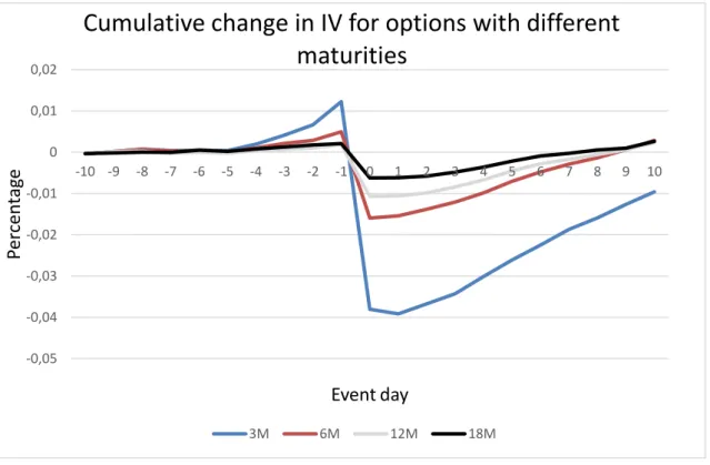
Figure 1: Cumulative change in IV for options with different maturities
Figure 1. Cumulative change in implied volatility for options with varying maturities from day -10 to day 10 relative to the earnings announcements. The implied volatilities are obtained from Bloomberg software and are averaged between call and put options for each maturity.
Figure 1 is a graph that presents the cumulative changes in percentage terms of the implied volatilities from 10 days prior to the EA until 10 days post the announcement. It has four lines, each representing a maturity that ranges from 3 months to 18 months. All four maturities display an increasing IV up to the EA day1.
1 It is important to state that the data is controlled for after hours announcements. Since the data of
the IV is based on the closing price, for any announcement made after hours, the day 0 will be the following day. For example, if the EA is made at 01/01/2010 at 12pm, the day considered 0 is 02/01/2010. This adjustment is necessary because as (Berkman and Truong (2009)) show, the after-hours EA are becoming more frequent.
-0,05 -0,04 -0,03 -0,02 -0,01 0 0,01 0,02 -10 -9 -8 -7 -6 -5 -4 -3 -2 -1 0 1 2 3 4 5 6 7 8 9 10 P er cen tag e Eventday
Cumulative change in IV for options with different
maturities
15 However, there is a considerable decrease on the following day, which makes the IV even less than day -10.
As it is shown on the figure 1, the IV starts to increase from day 1 to day 3 at a modest rate and then further accelerates until it reaches the previous levels observed at day -10. This could imply that there is some uncertainty prevalence after the announcement as agents try to access the true impact of the earnings. It could also mean that the stock price adjusted to what the investors consider to be the equilibrium price which makes the option IV return to the long-term value “agreed” among investors. We can also notice that the lower the maturity of the option, the higher the impact on implied volatility of the EAs both for the increases and decreases. This suggests that the EAs shock may be temporary and not prevail in the long term.
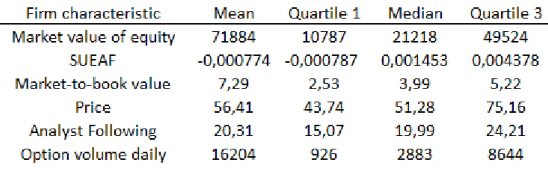
Table 2: Descriptive Statistics
This table presents descriptive statistics for the sample studied. The market value of equity is presented in ($ million) and is the year end values. SUEAF is the actual earnings minus expected earnings proxied by the mean of analysts’ forecasts scaled by the stock price at quarter end. Market-to-book value is the ratio of the firm’s market value to shareholder value of equity. Stock price is the year end average stock prices. The analyst following is the average number of analysts that provide earnings forecasts for the quarter announcements. Option volume is the average daily volume of options traded, both puts and calls.
The table 2 shows some characteristics of the sample used in this study. The average market value of equity is $71,9 billion but the median is $21,2 billion
16 indicating that the sample has some firms with unusual high market valuation which leads to a positive skew in what regards firm size. This is expected since the S&P500 is an index that hold the largest American companies ranking in market capitalization.
The mean of the SUEAF is -0,000774 and the median is 0,001453. The first quartile has a value very close to the mean of -0,000787 which indicates that there are some significant negative earnings surprises. The unexpected crisis of 2008 may explain a part of this occurrence. Other explanation might be that the firms usually avoid negative earnings surprises that are close to the expectations of the analysts according to Hayn et al (2002). They further find that companies favor posting considerable negative EAs when it is inevitable, giving out all the unexpected bad information to the market at once. This might be one reason why some considerable negative EAs may produce a distribution with a negative skew. The observation of few values representing earnings that fail to meet analyst expectations might impact the results because of the low representation in the sample.
The mean of Market-to-book value is 7,29 and the average price of the stocks of the sample is $56,41 which is considerably high and expected given that the sample comes from the S&P 500.
Since the S&P 500 is quite famous, the number of analysts following the constituent’s firms is also relatively high. In accordance with Zhu et al (2017) who found that if a security is added to an index the number of analysts following that security tends to increase. This number is further boosted because optioned firms tend to be followed by more analysts as Skinner (1990) proves. We end up with the average number of analysts following a firm of 20, with the first quartile being 15 and the third 24. The number of analysts’ is considerably high and provides a good sense of the overall expectations (opposed to few analysts following the stock, which could lead to a higher impact of outlier expectations).
17 The average daily volume of options traded is 16204, which is positively affected by some outlier firms that have a huge daily number of traded options.
5. Empirical results
5.1. Changes in implied volatility right after the
announcement
Table 3: Change in IV from day -1 to day 2
This table presents the change of the IV of the options from day -1 to day 2, relative to the EA date (which is day 0). The IV was extracted from Bloomberg and averaged out between calls and puts of the same maturity and strike price.
Table 3 shows the changes in implied volatility over a 3-day window (from day -1 to day +2) being the day 0 the EA date. The objective is to show the magnitude of the uncertainty resolution over a short-term period. On the first column the different maturities of the options studied are displayed. The second column displays the change in the implied volatility from the day prior to the EA (day -1) to the second day after the announcement (day +2). Analyzing the table, we find that the shorter the maturity of the option, the more pronounced is the decrease of the IV. The larger drop in IV is the 3M maturity options with a decrease of 4,9% and the smaller drop is the 18M maturity options with a decrease of 0,079%. With these results, the EAs seem to create a transitory change in the observed IV (a temporary increase in IV before the announcement followed by a decrease in the
18 IV right after the announcement). This effect was also found is several studies as for example Truong et al (2012). However, the change seems to dissipate over a larger time horizon, as Isakov & Pérignon (2001) shown, the IV takes several days to return to the long-term level. Ederington Lee (1996) findings are in line with the results on table 3 regarding the impact of scheduled announcements, where they are more pronounced on short maturity options in contrast to longer maturity options.
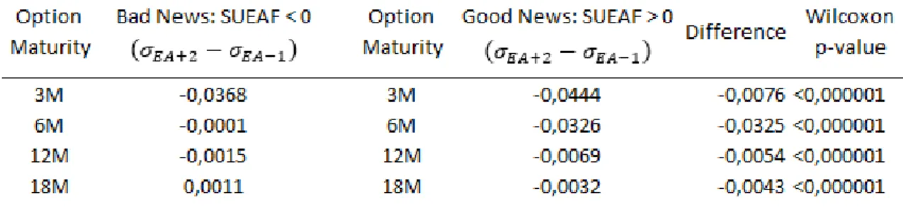
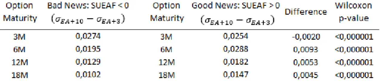
Table 4: Change in IV from day -1 to day 2 across maturity
This table presents the change of the IV of the options, separating by option maturity, and whether the SUEAF is positive or negative. The range of the difference is from day -1 to day 2, relative to the EA date (which is day 0). SUEAF is actual earnings minus expected earnings proxied by the mean of the most updated to date analysts’ forecasts divided by the stock price at the end of the quarter. The IV was extracted from Bloomberg and averaged out between calls and puts of the same maturity and strike price.
On table 4 the differences between the good and bad EAs are presented, using the measure of the SUEAF. Good EAs are defined as companies’ earnings per share equal or higher than average analysts’ forecasts (SUEAF ≥ 0). The bad EA’s are defined as companies’ earnings per share lower than average analysts’ forecasts (SUEAF < 0). To access whether the results are statistically significant, I used the wilcoxon signed-rank test which consists of repeated measurements on a single sample to assess whether the population mean ranks differ. It is a nonparametric
19 test and can be used when the population cannot be assumed to be normally distributed.
The decline in the IV is higher on good new announcements comparing to bad news announcements. The higher decline in IV in the SUEAF ≥ 0 is -4,44% which corresponds to the shorter maturity (3 months) and the lower decline is -0,32% which corresponds to the higher maturity (18 months). In what regards bad news, the higher decline of IV is -3,68% that corresponds to the 3 months maturity options and the lowest is the 6 months maturity options with an insignificant value of 0,01%. This might suggest that bad earnings surprises do not mitigate uncertainty in what regards long term horizons. As the results obtained regarding SUEAF ≥ 0 are more significant, good news might be associated with larger uncertainty resolution. Only short-term options (3 months maturity) reflect uncertainty resolution in bad earnings surprises.
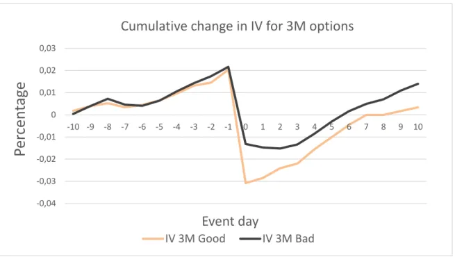
Figure 2: Cumulative change in IV for 3M options
This figure displays the cumulative change in implied volatility of 3 months to maturity options. The good and bad news earnings announcements are discriminated. The lower axis shows the days around the event day (EA). The “IV 3M Good” stands for the cumulative changes in percentage terms of the options’ IV
-0,04 -0,03 -0,02 -0,01 0 0,01 0,02 0,03 -10 -9 -8 -7 -6 -5 -4 -3 -2 -1 0 1 2 3 4 5 6 7 8 9 10
P
er
ce
n
tage
Event day
Cumulative change in IV for 3M options
20 (starting at day -10) of 3-month maturity options with SUEAF ≥ 0. The “IV 3M Bad” stands for the cumulative changes in percentage terms of the options’ IV (starting at day -10) of 3-month maturity options with SUEAF < 0. SUEAF is actual earnings minus expected earnings proxied by the mean of the most updated to date analysts’ forecasts, divided by the stock price at the end of the quarter. The IV was extracted from Bloomberg and averaged out between calls and puts of the same maturity and strike price.
Figure 2 is a display of the cumulative changes in the implied volatilities of the options with 3 months to maturity, with a distinction between bad and good announcements. The building up of the IV from the day -10 to -1 is steady. It reaches its peak, which is in day -1, to nearly 2% both for the good and bad EAs. One interesting factor is that the peak of the IV on day -1 doesn’t seem different between the two kinds of news. This could imply that the surprises are indeed surprises and traders do not seem to adjust the option pricing between good and bad news. If private information content was represented in the option pricing the IV would be expected to be higher on the day prior to bad news when compared to a day prior to good news. Campbell & Hentschel (1992) support this thought as they find that bad news are associated with higher volatility of the stock.
On day 0 the drop in the IV is more pronounced for good news rather for bad news announcements. The drop under SUEAF ≥ 0 is roughly -3% from the long-term values and the SUEAF < 0 is only about 1,5%. One difference between good and bad surprises is that the IV regarding good EAs starts to pick up to the long-term values on day 1 opposed to the bad EAs that prevails on the lowest levels for around 3 days. On the final day of the figure we can see that the final value of the cumulative IV is different. The options that traded on EA days with SUEAF ≥ 0 seem to have the IV similar to their long-term values, the IV of the options with SUEAF < 0 increased to values higher than the long-term value. This could imply that bad EAs bring uncertainty to the markets as investors expect higher volatility throughout the life spawn of the option.
21
5.2. Pre and post earnings announcement changes taking
into consideration news content.
Table 5: Change in IV from day 3 to day 10 across maturity
This table presents the change of the IV of the options separating by option maturity and whether the SUEAF is positive or negative. The range of the difference is from day 3 to day 10, relative to the EA date (which is day 0). SUEAF is actual earnings minus expected earnings proxied by the mean of the most updated to date analysts’ forecasts divided by the stock price at the end of the quarter. The IV was extracted from Bloomberg and averaged out between calls and puts of the same maturity and strike price.
Table 5 shows the differences between the good and bad EAs, using the measure of the SUEAF. The table shows insights of the post-announcement period (from day +3 to day +10). In all the maturities shown there is no prevalence of the low IV values recorded just after the EAs. This could mean that, for the presented maturities, the EAs do not bring enough uncertainty resolution to reduce the long-term values of the IV traders agree on the option pricing. The highest IV recovery can be found in the 3 months maturity options, which is expected, based on table 4 where we find that the shorter maturity options have the most significant decrease in IV. The results are statistically significant in all maturities. Making a cross analysis with table 4, for the results where the SUEAF was < 0 and the difference was minimal (6, 12 and 18 months), we can see on table 5 that all IVs increase by at least 1 percentage point. (1,95% for the 6-month maturity, 1,29% for the 12-month maturity and 1,02% for the 18-12-month maturity). This means that the IV for
22 those options increases until the end of the studied period, ending up with values higher than day -10. This finding will be more evident on table 6.
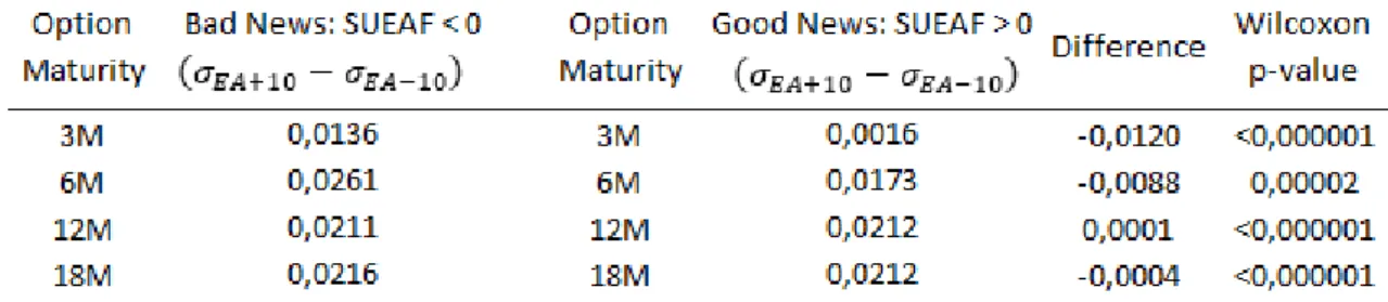
Table 6: Change in IV from day -10 to day 10 across maturity
This table presents the change of the IV of the options separating by option maturity and whether the SUEAF is positive or negative. The range of the difference is from day -10 to day 10, relative to the EA date (which is day 0). SUEAF is actual earnings minus expected earnings proxied by the mean of the most updated to date analysts’ forecasts divided by the stock price at the end of the quarter. The IV was extracted from Bloomberg and averaged out between calls and puts of the same maturity and strike price.
In table 6 we try to analyze the changes in long term IV of the options for each kind of news (good or bad). Truong et al (2012) found in their work that roughly on the day 10 after the announcement, the IV stabilizes to the long term value. This enables me to make a comparison between the day -10 and the day 10 in relation to the announcement and observe the impact on the long term changes in IV. Good EAs are defined as companies’ earnings per share equal or higher than the analysts’ mean forecasts (SUEAF ≥ 0). The bad EA’s are defined as companies’ earnings per share lower than average analysts’ forecasts (SUEAF < 0). The test is made by making the comparison between the IV on the first day of the time series (𝜎𝐸𝐴−10) and the last (𝜎𝐸𝐴+10).
The highest IV change can be found in the 6-month maturity options under bad EAs (+2,61%) and the lowest in the 3-month maturity options under good EAs (+0,16%). In what regards SUEAF ≥ 0 It seems that the lower the maturity the
23 lower the difference in long term implied volatility. This could suggest that uncertainty mitigation is negatively correlated with the maturity of the options. As for SUEAF < 0 the IV from day -10 to day 10 seems to increase significantly in all maturities presented.
The differences between good and bad announcements on the 3-month maturity options are the ones that display the higher change. On average, an option which the underlying had a bad EA, will see by day 10 an increase in the IV of 1,2% higher than an option which the underlying reports good EAs. The difference reported seems to decrease as maturities increase, and the 12-month and 18-month options data only shows insignificant differences. This could imply that for longer maturities the accounting earnings don’t play a significant role in the expectations of analysts as they try to access more meaningful information from the announcement. For example they could be more interested in the management earnings call, revenues expectations, macroeconomic trends, etc. Other possible explanation could be the fact that there are still a few catalysts until the maturity of the option (other earnings announcements). This seems to be the explanation for the huge differences reported between the 3 months maturity options and the others.
Throughout all the tables it is evident that the information content of accounting earnings cannot be ignored, as it impacts option valuation and IV. Options also seem to provide useful information about the impact of the EAs on the expectations of analysts about the future.
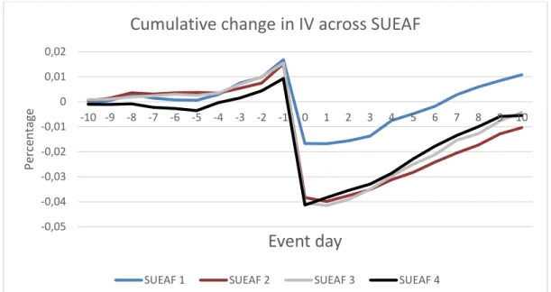
24 Figure 3: Cumulative change in IV across SUAEF
This figure presents cumulative changes in percentage terms of implied volatility for options with 90 days to maturity across quartiles of SUEAF. The SUEAF 1 presents the lowest quartile and SUAEF 4 the highest quartile. The range of the cumulative change in implied volatility is from day −10 to day +10 relative to the earnings announcements. SUEAF is actual earnings minus expected earnings proxied by the mean of the most updated to date analysts’ forecasts divided by the stock price at the end of the quarter. The IV was extracted from Bloomberg and averaged out between calls and puts of the same maturity and strike price. The data displayed is also adjusted for the movements of the S&P 500 to isolate the security specific volatility from the market movements.
Figure 3 graphically depicts the results regarding the cumulative change in implied volatility for options with 3-months to maturity by quartiles of SUEAF. Just like figure 1 and 2 there is an increase of the implied volatility until the announcement day across all quartiles. However, the drop in the IV is different and show, once again, some differences.
The first quartile seems to have the less pronounced drop, accounting for roughly -2% of the IV long term value. The rest of them decline to values close to -4%. The
-0,05 -0,04 -0,03 -0,02 -0,01 0 0,01 0,02 -10 -9 -8 -7 -6 -5 -4 -3 -2 -1 0 1 2 3 4 5 6 7 8 9 10 Pe rce n ta ge
Event day
Cumulative change in IV across SUEAF
25 recovery process is also different across the quartiles. To better understand this difference table 7 is plotted.
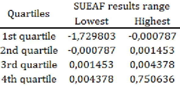
Table 7: SUEAF quartiles 3M options
This table presents the range of scores that SUEAF takes for each quartile. SUEAF is actual earnings minus expected earnings proxied by the mean of the most updated to date analysts’ forecasts divided by the stock price at the end of the quarter. As it is evident on table 7, the sample is dominated by positive SUEAF values (72,11% seen in the data step, table 1). The first quartile is completely dominated by bad earnings surprises which could explain the smallest drop of IV on the event day (in figure 3). This finding is in accordance with what has been written by Isakov & Pérignon (2001), where they state that the drop of IV recorded at day 0 is more pronounced with good news rather than bad. One interesting factor that is displayed on figure 3 is that the IV of the 1st quartile options seem to bring the long
term IV roughly 1% higher than the long-term average. This result is similar to the one found on table 6. Another interesting plot is the 2nd quartile. The value of the
IV for this line on the day 10 is the lowest one. This implies that under the 2nd
quartile there was more uncertainty resolution comparing to the others. This is an expected result with accordance of the findings of Campbell & Hentschel (1992). They explained that if companies bring bad news to the market, the volatility of the underlying will increase. However, if the firms bring surprisingly good news to the market there is also a spike in volatility as traders try to access how good the news are and what is the correct price of the stock. They concluded that the kinds of announcements that bring more resolution to the markets are the ones that meet the analysts’ expectations. As the second quartile has values between -0,000787 and 0,001453, the earnings in this interval are the ones that are closest to the
26 mean of analyst’s forecasts, when comparing to the other quartiles. This means that these EAs meet more precisely the analysts’ expectations, and we can observe that they reduced uncertainty the most. Both the third and fourth quartile seem to behave the same way, having a 4% drop on day 0 of IV and returning to their long-term values on day 10. It could mean that the investor uncertainty is not much affected by how good the news are, as long as they have a SUEAF higher than 0. Overall, the positive earnings seem to provoke the largest drop in IV comparing to bad EA. Thus, the impact of positive earnings news on option implied volatility appears more than just transitory.
As figure 3 shows, accounting earnings seem to have a great impact on the options pricing, more pronounced than just the underlying pricing. This supports the argument that options are no redundant securities and are rich in information content.
5.3. Limits in testing
5.3.1. Liquidity
One limitation in my study is the liquidity of the options traded. It is known that options are less traded than the underlying stocks and some companies enjoy lots of liquidity in what regards options, comparing to others as Truong & Corrado (2009) find. This is evident in the data step where the daily volume of options traded studied sample mean is higher than the 3rd quartile. (16204 opposed to
8644).
5.3.2. Outliers
The tests presented take out 0,5% of each tail of the distribution, to control for abnormal IV increases and decreases led by other factors different from the EAs. The choosing of the percentage of results to be taken from se sample (0,5%) was made according to previous studies such as Truong et al (2012).
27 5.3.3. Problems with the definition of good and bad news
Although this study is based on accounting earnings where the evaluated metric are the quarter EPS, it is important to remember that it is only a fraction of the news content of the EAs. This could mean that there is information which is released on the event day that is not incorporated in the definition of good / bad news. For example, if a company has a $2 EPS against the market consensus of $1.5, but the revenues were almost all made on credit and not cash payments, the analysts might regard it as bad news, where in my study it is considered good news. Therefore, some option prices might react from factors external to accounting earnings.
5.3.4. Defining the event day (day 0)
The data is controlled for after-hours announcements. Since the data of the IV is based on the closing price, for any announcement made after hours, the day 0 will be the following day. For example, if the EA is made at 01/01/2010 at 12pm, the day considered 0 is 02/01/2010. This adjustment is necessary because as Berkman and Truong (2009) show, the after-hours EA are becoming more frequent. Also, if there was no announcement there would any information resolution, meaning that only when the earnings are known, the analysts can react to them.
6. Conclusions
The studied theme of the impact of accounting earnings on equity and bonds has been receiving fair attention from the scholars. However the impact of the accounting earnings on the option pricing has not been studied so extensively. This study tries to bring a contribution to this less approached area of finance. I have examined the options’ market response in a short time window before and after the EAs. I isolated the IV to further understand the concerns of the investor in what regards uncertainty. As IV is the only variable that traders can control in the Black
28 Scholes formula (in exception to some extent the underlying price), it brings high levels of information in what regards the investor expectations.
I have found that the EA has a great impact on the option pricing driven by the changes in IV.
The first topic studied was the dynamics of the IV on a short time window after the EA date. I focused on two components: (1) an overall decline in IV explained by the resolution of uncertainty, and (2) the differences in the IV resolution between good and bad news (separated by the measure of the SUEAF). Although the first component has been fairly studied in the financial literature, the second one has still a lot of topics and methods to be explored.
The first hypothesis of this study was: “The information content of the earnings announcement may lead to a drop on implied volatility on the 3 following days after the announcement”. I have found that there seems to be an inverse relation in the change of the IV in a short window after the earnings announcements.
In what regards the kind of EAs the drop of IV, it seems to be less pronounced the worse the news announcements are. And, consequently, more pronounced the better the news announcements are. This suggests that good news erase more uncertainty from the market than bad news. This answers the second hypothesis “The drop in IV on the day after the earning announcement may have a higher magnitude if there is a good earnings announcement compared to a bad earnings announcement”. For some levels, the bad news actually ended up bringing more volatility to the market.
Other finding was that the higher the maturity of the option the less pronounced this drop in IV is. This might suggest that, for longer maturities, investors seem to give less importance to the accounting earnings of the period. But, overall, the accounting earnings seem to have impact on both the short and the long term (with higher impact on the short term).
29 In what regards the long term IV effect there are also some interesting findings. As good news seems to bring the uncertainty down for longer periods, bad news usually brings uncertainty to values higher than the long term. This effect is positively related to the maturity of the options. These findings meet the ones done by Veronesi & Pastor (2003) where they state: “uncertainty regarding a firm’s profitability is increasing in idiosyncratic volatility”. The results also seem to be in accordance with the leverage effects extensively studied by Black (1976). In what regards the pre announcement period, the options’ IV do not increase in anticipation of Bad EAs. This could imply that there is no inside information taken into consideration in the pricing of the options. As Campbell & Hentschel (1992) find, bad EAs seem to be associated with higher volatility of the stock. For that reason, if inside information was priced on the calls, it would be expected that the cumulative increase of the IV would be higher on day -1 for the stocks that were going to announce earnings that fail to meet analysts’ expectations. As the values on day -1 of the cumulative IV seem to be equal, traders do not seem to anticipate bad news.
The results in this work in what regards the relation between the IV, EA and kinds of news could suggest that there is still a lot to be studied in this three factor relation. One example of further research would be: to study the IV on interest rates options where the announcement date is the central bank scheduled interest rate announcements. It could bring rich information about investor expectations as financial markets are increasingly more affected by the central banks announcements (especially after the 2008 crisis).
7. References
Amin, K. and C. Lee. 1997. Option trading and earnings news dissemination. Contemporary Accounting Research 14 (2), 153-192.
30 Back, K., 1993. Asymmetric information and options. Review of Financial Studies 6, (3) 435–472.
Ball, R. and Brown, P., 1968. An empirical evaluation of accounting income numbers. Journal of Accounting Research 6 (2), 159–178
Bartov, E., Radhakrishnan, S. and Krinsky, I., 2000. Investor sophistication and patterns in stock returns after earnings announcements. The Accounting Review 75, (1) 43–63.
Basu, S., 1997. The conservatism principle and the asymmetric timeliness of earnings. Journal of Accounting and Economics 24 (1), 3–37.
Beaver, W.H., 1968. The information content of annual earnings announcements. The Journal of Accounting Research 6 (3), 67–92.
Berkman, H. and Truong, C., 2009. Event day 0? After-hours earnings announcements. Journal of Accounting Research 47 (1), 71–103.
Biais, B. and Hillion, P., 1994. Insider and liquidity trading in stock and options markets. Review of Financial Studies 7, (4) 743–780.
Black, F. and Scholes, M., 1973. The valuation of options and corporate liabilities. Journal of Political Economy 81, (1) 637–654.
Black, F.,1976. Studies of stock price volatility changes. In: Proceedings of the 1976 Meetings of the American Statistical Association. Business and Economics Statistics Section.
Brown, K., Harlow, W. and Tinic, S. 1988. Risk aversion, uncertain information, and market efficiency. Journal of Finance (2), 355-385
Campbell, J.Y. and Hentschel, L., 1992. No news is good news: an asymmetric model of changing volatility in stock returns. Journal of Financial Economics 31 (3), 281– 318.
31 Cao, H. 1999. The effect if derivative assets on information acquisition and price behavior in a rational expectations equilibrium. Review of financial studies 12, (1) 131-163.
Christie, A.A., 1982. The stochastic behavior of common stock variances: value, leverage and interest rate effects. Journal of Financial Economics 10, (4) 407–432. Cohen, Lee,. Alan, Marcus,. Rezaee, Zabihollah,. Tehranian, Hassan, 2018. Waiting for guidance: Disclosure noise, verification delay, and the value-relevance of good-news versus bad-good-news management earnings forecasts. Global finance Journal, Volume 37, 79-99.
Conrad, J. 1989. The price effect of option introduction. The journal of finance. (2), 487-498.
Cornell, B., 1978. Using the option pricing model to measure the uncertainty-producing effect of major announcements. Financial Management 7 (1), 54–59. Cremers, M., and D. Weinbaum. 2010. Deviations from put call parity and stock return predictability, Journal of Financial and Quantitative Analysis 45, (2) 335-367.
Cremers, M. and Fodor, A. and Weinbaum, D. 2017. Where do informed traders trade first? Option trading activity, news releases and stock return predictability. SSRN Electronic Journal.
Detemple, J. and Selden, L., 1991. A general equilibrium analysis of option and stock market interactions. International Economic Review 32 (2), 279–304.
Donders, M.W.M., Vorst, T.C.F., 1996. The impact of firms specific news on implied volatilities. Journal of Banking and Finance 20, (9) 1447–1461.
Donders, M.W.M., Kouwenberg, R., Vorst, T.C.F., 2000. Options and earnings
announcements: an empirical study of volatility, trading volume, open interest and liquidity. European Financial Management 6 (2), 149–171.
32 Easley, D., O’Hara, M. and Srinivas, P.S., 1998. Option volume and stock prices: evidence on where informed traders trade. Journal of Finance 53 (2), 431–465 Ederington, L.H., Lee and J.H., 1996. The creation and resolution of market uncertainty: the impact of information releases on implied volatility. Journal of Financial and Quantitative Analysis 31, (4)513–539
Ederington, L.H. and Goh, J.C., 1998. Bond rating agencies and stock analysts: who knows what, when? Journal of Financial and Quantitative Analysis 33 (4), 569–585. Fama, F. and MacBth, D. 1970. Risk, Return and Equilibrium: Empirical tests. Chicago Journals (3), 607-636.
French, K.R., Schwert, G.W. and Stambaugh, R.F., 1987. Expected stock returns and volatility. Journal of Financial Economics 19 (1), 3–30.
Foster, G., Olsen, C. and Shevlin, T., 1984. Earnings releases, anomalies, and the behavior of security returns. The Accounting Review 59 (4), 574–603.
Fu, Xi and Arisoy, Y. Eser and Shackleton, Mark Broughton and Umutlu, Mehmet. 2016. Option implied volatility measures and stock return predictability. Journal of Derivatives, 24 (1). pp. 58-78
Goh, J.C. and Ederington, L.H., 1993. Is a bond rating downgrading bad news, good news, or no news for stockholders? Journal of Finance 48 (5), 2001–2008.
Hayn, C., Givoly, D, and Bartov, E. 2002. The rewards to meeting or beating earnings expectations. Journal of accounting and economics, 33 (2), 173-204. Hong, H. and Stein, J. 1999. A unified theory of underreaction, momentum trading, and overreaction in asset markets. The journal of Finance (6), 2143-2184.
Isakov, D. and Perignon, C., 2001. Evolution of market uncertainty around earnings announcements. Journal of Banking and Finance 5 (9), 1769–1788.
33 Jennings, R. and Starks, L. 1986. Earnings announcements, stock price adjustment, and the existence of option markets. The journal of finance (1) 107- 125.
Kasnik, R. and McNichols, M.F., 2002. Does meeting earnings expectations matter? Evidence from analysts forecast revisions and stock prices’. Journal of Accounting Research 40 (3), 727–759.
Latané, R. and Rendelman, R., 1976. Standard deviations of stock prices ratios implied in option prices. Journal of Finance 31 (2), 369–381.
Lee, C., Mucklow, B. and Ready, M., 1993. Spreads, depths and the impact of earnings information. Review of Financial Studies (6), 354–376.
Lipe, R.C., Bryant, L. and Widener, S.K., 1998. Do nonlinearity, firm-specific coefficients, and losses represent distinct factors in the relation between stock returns and accounting earnings? Journal of Accounting and Economics 25 (2), 195–214.
Livnat, J. and Mendenhall, R.R., 2006. Comparing the post-earnings announcement drift for surprises calculated from analyst and time series forecasts. Journal of Accounting Research 44 (1), 177–205
MCQueen, G., Pinegar, M. and Thorley, S. 1996. Delayed reaction to good news and the cross-autocorrelation of portfolio returns. The journal of Finance, (3) 889-919. Ni, S., J. Pan, and A. Poteshman. 2008. Volatility information trading in the option market. Journal of Finance 63: 1959-1092.
Nofsinger, J. 2001. The impact of public information on investors. The journal of banking and finance, (7) 1339-1366.
Pan, J., Poteshman, A. 2006. The information in option volume for future stock prices. Oxford university press, (3) 871-908.
Pastor, L., Veronesi, P., 2003. Stock valuation and learning about profitability. Journal of Finance (58), 1749–1790.
34 Patell, J.M. and Wolfson, M.A., 1979. Anticipated information releases reflected in call option prices. Journal of Accounting and Economics 1 and 2, 117–140
Patell, J.M. and Wolfson, M.A., 1981. The ex-ante and ex-post price effects of quarterly earnings announcements reflected in option and stock prices. Journal of Accounting Research (2), 434–458.
Rogers, J.L., Skinner, D.J. and Van Buskirk, A., 2009. Earnings guidance and market uncertainty. Journal of Accounting and Economics 48 (1), 90–109.
Schwert, G.W., 1989. Why does stock market volatility change over time? Journal of Finance 44 (5), 1115–1154.
Skinner, J. 1989. Option markets and stock return volatility. Journal of Financial Economics, (1) 61-78.
Skinner, J. 1990. Options markets and the information content of accounting earnings releases. Journal of accountings and Economics, (1) 191-211.
Tuan, Q., Norman, Strong., Martin, Walker. 2018. Modelling analysts’ target price revisions following good and bad news? Jounal of ccounting and business research. Issue 1, Volume 48. 37-61.
Truong, C., Corrado, C. and Chen, Y. 2012. The options market response to accounting earnings announcements. Journal of International Financial Markets, Institutions & Money. 423-450.
Xing, Y.H., Zhang, X.Y. and Zhao, R., 2010. What does individual option volatility smirk tell us about future equity returns? Journal of Financial and Quantitative Analysis 45, (3) 641–662.
Zhu, S., Jiang, X., Ke, X. and Bai, X. 2017. Stock index adjustments, analyst coverage and institutional holdings: Evidence from China. China journal of Accounting Research, (3) 281-293.