Analysis of the Thermal Performance of Opaque Building Envelope Components Using In situ Measurements

A

NALYSIS OF THE THERMAL

PERFORMANCE OF OPAQUE BUILDING

E

NVELOPE

C

OMPONENTS USING

IN SITU MEASUREMENTS

J

R

M

M

A dissertation submitted in partial fulfillment of the requirements for the degree of

MASTER IN CIVIL ENGINEERING —SPECIALIZATION IN BUILDING CONSTRUCTION

Supervisor: Prof. Dr. Nuno Manuel Monteiro Ramos

Tel. +351-22-508 1901 Fax +351-22-508 1446

 miec@fe.up.pt

Edited by

FACULTY OF ENGINEERING OF THE UNIVERSITY OF PORTO Rua Dr. Roberto Frias

4200-465 PORTO Portugal Tel. +351-22-508 1400 Fax +351-22-508 1440  feup@fe.up.pt  http://www.fe.up.pt

Partial reproductions of this document are allowed on the condition that the Author is mentioned and that the reference is made to Integrated Master in Civil Engineering – 2015/2016 – Department of Civil Engineering, Faculty of Engineering of the University of Porto, Porto, Portugal, 2016.

The opinions and information included in this document represent solely the point of view of the respective Author, while the Editor cannot accept any legal responsibility or other with respect to errors or omissions that may exist.

To my family

Life is about making an impact, not an income. Kevin Kruse

ACKNOWLEDGEMENTS

First and foremost, I want to thank Dr. Nuno Ramos, who since the first moment created all the conditions to complete this period abroad, accepting promptly to be my tutor but also for helping me taking care of all bureaucracies and sacrificing his time to help me.

I would also to acknowledge Prof. Dirk Saelens who allowed me doing my dissertation at KU Leuven. Without him, this amazing opportunity would not be possible.

A special thanks belong to Marieline Senave, Evie Lambie, and Glenn Reynders, the people who were always available to help me, spending their time explain and showing me everything to fully understand the subject and took care of me the whole time I was in Leuven. Thank you and all the best of luck in your future endeavors.

To all my friends that crossed my journey during this five years, a special thanks. I will remember forever in my heart the stories and the moments you shared with me.

To Lúcia Ferreira, who deserves my wholehearted thanks for giving me the motivation to reach for the stars and chase my dreams. Thank you for teaching me that my job in life was to learn, to be happy, and to love.

Last but not least, having the consciousness that alone this journey would not have been possible, my greatest thanks to my parents and sister for their unconditional love, support, and encouragement. Without their grace, this would have never been a reality.

ABSTRACT

On-site measurements carried out on new buildings evidence that the actual energy performance of a the as-built environment can deviate significantly from the one predicted by energy simulation tools or envisaged by the design expectations and in-use outcomes.

To meet the causes of this performance gap, it is essential that we can measure accurately how well our new homes are performing. Its thermal characteristics must be estimated and, to this aim different approaches are available. Those approaches include both field measurements and data analysis. One of the key parameters to describe the thermal performance of building envelope components is its components thermal transmittance, U-value, theoretically characterized by ISO 6946 or in-situ by Heat Flow Meter (HFM) measurements following the considerations of ISO 9869.

Through two residential houses where HFM measurements were performed, we characterize the U-value for the opaque elements of its envelope. Two different data analysis methodologies were applied, a nondynamical/ steady-state approach (Linear regression model) and a dynamical and stationary approach (Autoregressive with exogenous model – ARX model).

The results of the tests show a good behaviour of HFM measurements when performed under the conditions in ISO 9869. Moreover, both data analysis approaches presented accurate and consistent results for test experiments with stable and controlled quasi steady state conditions. The amount of collected data indicates more consistency and accuracy in the results.

KEYWORDS:In-situ measurements; Thermal performance; Thermal transmittance; U-value; Heat Flow Meter method; ARX modelling; Linear regression model.

RESUMO

A constante realização de testes in-situ evidencia em novos edifícios que o desempenho real de energia de edificações construídas pode desviar-se significativamente do previsto, quer por ferramentas e tecnologias de simulação de gastos de energia, quer pelas previstas durante a gestão de expectativas em projeto e mesmo devido á utilização dos seus utentes.

Para atender as causas dessa diferença de desempenho, é essencial medir com precisão o real e atual desempenho das mesmas. As suas características térmicas devem ser estimadas e, para este objetivo, diferentes abordagens e metodologias estão disponíveis. Essas abordagens incluem quer diferentes testes e medições de campo tal como diferentes metodologias para a consequente análise de dados. Um dos conceitos chave para descrever o desempenho térmico dos componentes da envolvente de um edifício, é o seu coeficiente de transmissão térmica, U-value, caracterizado teoricamente pela norma ISO 6946 ou in-situ através do Heat Flow Meter method (HFM) descrito na ISO 9869.

Através de dois casos de estudo, duas habitações na Bélgica, onde medições através de HFM foram realizadas, procedemos à caracterização do coeficiente de transmissão térmica para os elementos opacos das respetivas envolventes. Duas metodologias de análise de dados foram aplicadas; Uma abordagem estática (recorrendo à regressão linear como modelo utilizado) e uma abordagem dinâmica e estacionária (recorrendo ao modelo ARX - Autoregressive with exogenous model).

Os resultados dos testes mostram um bom comportamento de medições HFM quando realizada sob as condições da norma ISO 9869. Por outro lado, ambas as diferentes metodologias aplicadas para a respetiva análise de dados apresentam consistência nos resultados quando os ensaios são realizados sob condições controladas e quase estáticas. A quantidade de dados recolhidos indicam mais consistência e precisão nos resultados o que indica que ensaios com uma maior duração conduzem a maior precisão nos resultados.

KEYWORDS:In-situ measurements; Performance térmica; Coeficiente de transmissão térmica; U-value; Heat Flow Meter method; ARX model; Regressão linear; Análise de dados.

GENERAL INDEX ACKNOWLEDGEMENTS ... iii ABSTRACT ... vii RESUMO ... ix

1. INTRODUCTION

2. STATE OF THE ART

2.1.BUILDING ENVELOPE AND ITS RELEVANCE FOR BUILDING’S THERMAL PERFORMANCE ... 5

2.2.BUILDING ENVELOPE COMPONENTS:HEAT BALANCE ... 6

2.3.BUILDING ENVELOPE COMPONENTS:THERMAL CHARACTERISTICS DESCRIPTION ... 8

2.3.1.THERMAL INSULATION ... 9

2.3.2. THERMAL CONDUCTIVITY ... 9

2.3.3. THERMAL RESISTANCE:R-VALUE ... 10

2.3.4. THERMAL TRANSMITTANCE:U-VALUE ... 11

2.3.5. THERMAL MASS ... 12

2.4.WHOLE BUILDING ENVELOPE:THERMAL CHARACTERISTICS DESCRIPTION ... 13

2.4.1.OVERALL HEAT LOSS COEFFICIENT ... 13

2.4.2. AIRTIGHTNESS ... 13

2.5.TEST CAMPAIGNS ... 15

2.5.1.HEAT FLOW METER METHOD ... 15

2.5.2. INFRARED THERMOVISION TECHNIQUE ... 18

2.5.3. CO-HEATING TEST ... 22

2.5.4. TEST CAMPAIGNS VARIATIONS AND ADAPTIONS ... 26

2.6.TIME SERIES DATA ANALYSIS ... 27

2.6.1.SYSTEM ... 28

2.6.2. SYSTEM MODEL... 29

2.6.3. MODEL TYPES ... 29

2.7.1.LINEAR REGRESSION BASED MODELS ... 35

2.7.2. AUTOREGRESSIVE P-ORDER BASED MODELS ... 40

2.7.3. R-VALUE CHARACTERIZATION THROUGH LINEAR REGRESSION MODEL (STEADY STATE APPROACH) ... 42

2.7.4. R-VALUE CHARACTERIZATION THROUGH ARX MODEL (DYNAMICAL APPROACH) ... 44

3. TEST CASES DESCRIPTION

3.1.TERRACED HOUSE IN DESSEL,BELGIUM ... 47

3.1.1.DWELLING DESCRIPTION ... 47

3.1.2.TEST EQUIPMENT ... 48

3.1.3.EXPERIMENT DESIGN ... 49

3.2.TERRACED HOUSE IN BILZEN,BELGIUM ... 50

3.2.1.DWELLING DESCRIPTION ... 50

3.2.2.TEST EQUIPMENT ... 51

3.2.3.EXPERIMENT DESIGN ... 52

3.3.EXPERIMENT DESIGN DISCUSSION ... 53

4. U-VALUE CHARACTERIZATION

4.1.TEST CASE A:TERRACED HOUSE IN DESSEL,BELGIUM ... 55

4.1.1.DATA ANALYSIS APPROACH... 55

4.1.2.ESTIMATING U-VALUE USING LINEAR REGRESSION ... 55

4.1.3.RESULTS DISCUSSION ... 60

4.2.TEST CASE B:TERRACED HOUSE IN BILZEN,BELGIUM ... 61

4.2.1.DATA ANALYSIS APPROACH... 61

4.2.2.U-VALUE CHARACTERIZATION USING LINEAR REGRESSION ... 64

4.2.3.U-VALUE CHARACTERIZATION USING ARX MODELING ... 70

4.2.4.RESULTS DISCUSSION ... 73

5. CONCLUSIONS

5.1.MAIN CONCLUSIONS ... 75

5.2.FUTURE RESEARCH DIRECTIONS ... 77

REFERENCES

ANNEX 1

INDEX OF FIGURES

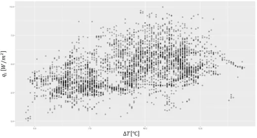
Fig.1 – The impact of measures to reduce building’s heat loss and heating demand ... 2 Fig.2 – Main factors which influence the building heat balance ... 6 Fig.3 – Heat transfer modes experienced by windows ... 8 Fig.4 - The influence of thermal mass on the periodic heat flow. The diurnal variations of the outdoor temperature (yellow line) result in heat flows into the building during the day, where part of the heat is stored in the material. During the night, the heat flow is reversed. ... 12 Fig.5 – Heat (left) and thermal (right) sensor plates... 16 Fig.6 – U-value estimation and its confidence interval from ITT method under different weather conditions. In 12 and 18-Fev: cloud cover, and wind speeds of resp. 1.4m/s and 0.3m/s during IR measurement, but still influence of long-wave radiation of the sky on the surface temperature. On 17-Fev: solar insolation on the facade during the measurement. On 21-17-Fev: at least 30 hours of heavy overcast before the measurement took place. ... 21 Fig.7 – Coheating test equipment during text experiments. ... 24 Fig.8 - Process from raw data to the full understanding of the test campaigns ... 27 Fig.9 – Elements that describe a system: Inputs and Outputs (databased elements) and the internal system processes ... 28 Fig.10 – Model types and its main differences: previous physical knowledge on the mathematical structure and the level of data dependency ... 29 Fig.11 – General procedure for time series data analysis. This approach was designed focusing especially in data collected from the experiments described in section 2.5. ... 32 Fig.12 – Brief illustration of the four assumptions to perform an linear regression ... 38 Fig.13 – On the right there is a observable trend over time what represents the nonstationary of the data ... 41 Fig.14 – Test case A. Single family dwelling in Dessel, Belgium ... 47 Fig.15 – Heat flux plate and temperature cell in internal environment (left);Temperature cell in the exterior (right) ... 49 Fig.16 – Test case B. Single family dwelling in Bilzen, Belgium ... 50 Fig.17 – Left: Heat flux plate and temperature cell in internal environment, located far enough from openings and the cross between walls. In the right the data logger used for temperature readings .... 52 Fig.18 – Methodology applied for each estimation from raw data to results validation ... 55 Fig.19 – Test Case A: Front façade. Raw data collected from the Test campaign. The red circles present some outliers ... 56 Fig.20 – Test Case A: Front façade. Raw data processed and filtered from the Test campaign ... 57 Fig.21 – Test Case A: Front façade. Time series plots of the filtered measurements ... 57

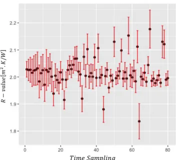
Fig.23 – Test Case A: Front façade. R-value tendency over a time sampling from 1 to 80 hours ... 59

Fig.24 – Test Case A: Front façade. Auto-correlation plot of the residuals and Cross-correlation plot to the inputs ... 59

Fig.25 – Test Case A: Rear façade. Time series plots of the filtered measurements. ... 60

Fig.26 – Test Case A: Rear façade. R-value tendency over a time sampling from 1 to 80 hours. ... 60

Fig.27 – Test Case B: Front façade. Raw data processed and filtered from the Test campaign ... 63

Fig.28 – Test Case B: Front façade. Time series plots of the filtered measurements ... 63

Fig.29 – Test Case B: Back façade. Raw data processed and filtered from the Test campaign ... 64

Fig.30 – Test Case B: Back façade. Time series plots of the filtered measurements. ... 64

Fig.31 – Test Case B: Front façade. Time series plots of the filtered measurements considering a period of 2 weeks [10th _{to 24}th _{January] ... 65}

Fig.32 – Test Case B: Rear façade. Time series plots of the filtered measurements considering a period of 2 weeks [10th _{to 24}th _{January] ... 66}

Fig.33 – Test Case B: Front façade. Time series plots of the filtered measurements considering a period of 6 days [10th _{to 16}th _{January] ... 67}

Fig.34 – Test Case B: Rear façade. Time series plots of the filtered measurements considering a period of 6 days [10th _{to 16}th _{January] ... 68}

Fig.35 – Test Case B: Front façade. R-value tendency for different sample time[from 1 to 80 hour ... 68

Fig.36 – Test Case B: Rear façade. R-value tendency for different sample time from 1 to 80 hour ... 68

Fig.37 – Test Case B: Front façade. R-value estimation with 95% confidence interval over different Time Sample ... 69

Fig.38 – Test Case B: Rear façade. R-value estimation with 95% confidence interval over different Time Sample ... 69

Fig.39 – Test Case B: Front (above) and Rear (bellow) façade. R-value estimation with 95% confidence interval over different periods for a time sample of 24 hours ... 70

Fig.40 – Test Case B: Front façade. R-value estimation with 95% confidence interval over different time samples ... 72

Fig.41 – Test Case B: Rear façade. R-value estimation with 95% confidence interval over different time samples ... 72

Fig.42 – Test Case B: Front façade. R-value estimation with 95% confidence interval over different data subsets ... 73

Fig.43 – Test Case B: Rear façade. R-value estimation with 95% confidence interval over different data subsets ... 74

INDEX OF TABLES

Table 2.1 – Heat Flow meter method: advantages and disadvantages ... 18

Table 2.2 – ITT method: advantages and disadvantages ... 22

Table 2.3 – Co-heating test: advantages and disadvantages ... 26

Table 2.4 – Black-box models: advantages and disadvantages ... 30

Table 2.5 – White-box models: advantages and disadvantages ... 30

Table 2.6 – Linear regression based models: advantages and disadvantages ... 39

Table 2.7 – Autoregressive p-order based models: advantages and disadvantages ... 42

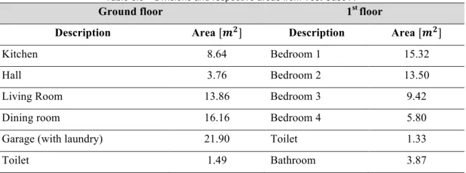
Table 3.1 – Divisions and respective areas from Test Case A ... 48

Table 3.2 – Materials of the opaque building envelope components and its respective characteristics. The constitution of the three external walls is the same ... 48

Table 3.3 – Test case A: Summary of measurements(Front façade) ... 50

Table 3.4 – Test case A: Summary of measurements(Rear façade) ... 50

Table 3.5 – Divisions and respective areas from Test Case A ... 51

Table 3.6 – Test case B: Summary of measurements(Front façade) ... 52

Table 3.7 – Test case B: Summary of measurements(Rear façade) ... 53

Table 4.1 – Test Case A: Front façade. Summary of the time series filtered ... 58

Table 4.2 – Test Case A: U-value final estimation through simple linear regression ... 61

Table 4.3 – Test case B: data approach ... 62

Table 4.4 – Test Case B: Front façade. Summary of the time series ... 63

Table 4.5 – Test Case B: Back façade. Summary of the time series ... 64

Table 4.6 – Test Case B: Summary of the difference in temperature for different data subsets ... 67

Table 4.7 – Test Case B: Characterization of U-value over different test scenarios ... 71

SYMBOLS

Δ𝑇 – Indoor-Outdoor air temperature [K] 𝑉 – Internal volume of a building [m3_] 𝜌 – Density of a material [Kg/m3_] 𝑆 – Area [m2_]

𝜀 – Surface emissivity of an material [W/m2_K] 𝑙 – Thickness of a layer [m]

𝑅𝑠𝑖 – Internal surface thermal resistance [m2K/W] 𝑅𝑠𝑒 – External surface thermal resistance [m2K/W]

𝑇𝑠𝑖 – Internal surface temperature of a building component [K] 𝑇𝑠𝑒 – External surface temperature of a building component [K] 𝑇𝑖 – Internal environment (ambient) temperature [K]

𝑇𝑒 – External environment (ambient) temperature [K] 𝜆 – Thermal conductivity [W/m2_K]

Λ – Thermal conductance of a building component surface to surface [W/m2_K] 𝑈 – Heat Transfer coefficient [W/m2_K]

𝑅 – Thermal resistance [m2_K/W] 𝑞 – Density of Heat Flow rate [W/m2_] 𝜙 – Heat flow rate [W]

𝐻𝐿𝐶 – Overall heat loss coefficient [W/K] ∑ 𝐴𝑈 – Total transmission heat loss [W/K] 𝑐𝑎𝐺𝑎 – Ventilation heat loss [W/K]

𝑐 – Specific heat capacity of a material [J/Kg.K] 𝑐𝑎 – Specific heat capacity of air [J/Kg.K]

𝐺𝑎 – Natural airflow through building fabric [Kg/s] 𝜂50 – Air change rate at 50𝑃𝑎 [h]

1

INTRODUCTION

1.1. BACKGROUND

According to the UK National Energy Efficiency Action Plan of April 2014 (NEEAP), buildings are responsible for 40% of energy consumption and 36% of CO2 emissions in the EU, what represents the importance of the building sector to the energy use and greenhouse gas emission. For instance, when we look at the Horizon 2020, the biggest EU research and innovation program ever, and then at its structure, the EU has set five headline targets - on employment, innovation, education, social inclusion and climate/ energy. Focusing on the climate changes and energy improvements, the following objectives were defined:

§ Reduce greenhouse gas emissions by at least 20% compared to 1990 levels; § Increasing the share of renewable energy in final energy consumption to 20%; § Moving towards a 20% growth in energy efficiency.

As a result, research and demonstrations of more energy efficient technologies and solutions are being undertaken, and new standards are being imposed. The 2010 Energy performance of buildings directive (EPBD) states all new buildings must be nearly zero energy buildings by 31 December 2020 and for public buildings by 31 December 2018. However, “Most of the buildings that will exist in the year 2050 are already built. Renovation of the existing building stock is, therefore, the key to meeting our long-term energy and climate goals” (Moseley 2016, p.2). This underlines the importance in a special focusing on the refurbishment and renovation of the as-built environment. Then new standards, technologies, and the expertise level must go a step forward. An essential starting point for any improvement process is an accurate evaluation and characterization of the existing buildings. Detailing the real energetic performance of an existing building remains a challenge, and a gap from the design plans to real environment still be visible through the countless test campaigns easily found in the literature (Bauwens 2015). This evaluation and characterization procedure is a process that usually involves multiple disciplines and fields (Wu, 2016). Choosing the right parameters or the most suitable test protocol is often a difficult task since the building sector has not a uniform pattern. As said, one of the flagship goals of the Horizon 2020 is to reduce energy consumption and CO2 emissions of the building industry. Therefore, it is fair to focus on the heating/ cooling requirements on buildings.

Fig.1 – The impact of measures to reduce building’s heat loss and heating demand(Allen, Blake et al. 2013). As showed in Fig.1, acting on the building envelope can be one of the main and wiser decisions to focus, when we are thinking about reducing a building’s heat loss and heating demand.

1.2.SCOPE

In light of the evidence present on the picture Fig.1, improvements in the building envelope elements can reduce the buildings' heat demand up to 50%.

It is thus, important to have an ability accurately and reliably to measure the thermal performance of fabric elements in order to define a proper strategy to intervene in the as-built environment. The primary purpose of the present dissertation becomes then, to review the current best practices addressing both test set-up and data analysis. In order to address this idea we aim to focus in the following bullets:

§ Description of building envelope and its thermal properties, underlining its importance and role in the heat balance of a building;

§ Review over different approaches in order to evaluate in situ its thermal properties; Different test campaigns are illustrated and analyzed;

§ Review over different data treatment taking into account collected data during field measurements;

§ Highlight for both field test set-up and data analysis procedures theirs strengths and weaknesses.

Through the study of two residential houses in Belgium where full-scale measurements were performed, our major aim becomes:

thermal transmittance, U-value, of opaque building envelope components, through Heat Flux Measurements;

§ Analysis of different scenarios from collected data identifying possible improvements and practices design in order to increase the level of reliability of the applied test campaigns.

1.3.CHAPTERS OVERVIEW

The content of the present dissertation is organized in five chapters.

The introduction of the topic of the present dissertation as well its objectives and structure are addressed in the first chapter.

The second chapter contains the literature review of the current state of the art. It is presented in two parts. The first part concerning to the description of the physical phenomena behind heat flux through opaque building envelope elements. Secondly, test campaigns are revised, addressing both in situ test set-up and data analysis. For each approach are underlined important aspects to take into consideration, highlighting the main advantages and disadvantages of each in situ test experiments as well as data analysis methodologies.

The third chapter, "Test cases description", focuses on the characterization of both test cases describing the building envelope and its thermophysical characteristics as well as the strategy of the test campaign applied. In the first test case a Heat Flux Measurements was performed while in the second, we proceed as well to the analysis of an HFM campaign. However, in this case, the technique was performed simultaneously with a co-heating test.

Through the fourth chapter, we proceed to the characterization of the thermal transmittance, U-value of the building envelope components and the evaluation of the test experiments. We attempt as well through the analysis of the parameters estimation, evaluate the suitability of each test campaign stressing the main weaknesses encountered during the test campaigns and identifying possible improvements for future in situ measurements.

The fifth and final chapter presents general findings of the work here developed and some aspects that should be improved in further works on the current topic.

2

STATE-OF-THE-ART

2.1.BUILDING ENVELOPE AND ITS RELEVANCE FOR BUILDING’S THERMAL PERFORMANCE

When we face a building it is undoubtedly our first impression is related to its envelope, the physical barrier splitting the indoor and outdoor environments. It becomes imperative to underline its critical role as the most important component to reaching the desired comfort level of the users.

Building’s envelope is typically constituted by his opaque fabric components (walls, roofs, floors, doors, and ceilings) and his fenestrations (all types of openings in the structure as skylights, windows or clerestories). Its functions aim to meet a suitable robustness of the building, fit the user’s requirements and purposes and reduce life cycle costs (Sadineni, Madala et al. 2011). However, its central role is to perform as a critical component to fighting against the undesired (or take advantage of his) climatic and an environmental phenomenon of his location as air, noise, water, heat and light conditions.

Keep out the rain and noise from the indoor environment, control the heat losses and gains and air infiltrations or prevent moisture threats as internal condensation or moisture migration are important factors that must be taken into account since a careful design process. For instance, an incorrect or unsuitable building technologies selection cannot meet the heating and cooling requirements substantially increase the operating costs and also the dependence of building services and mechanical equipment, often expensive.

Fortunately, an optimal design can be easily achieved for new buildings. However, for older building there still great opportunities and possibilities to increase the performance of a building envelope reaching higher levels of efficiency. Upgrades at the fenestration level or doors or even at the finishing surface are the easiest options to perform a considerable upgrade on the building envelope efficiency. One last point is that an accurate design process will not be ensured through the desired levels of comfort and effectiveness. Decisions about in situ construction details and procedures, workmanship experience, or even user behavior also play a crucial role to ensure the efficiency of the building during its service life period.

Focusing especially on the influence of the building envelope to reach the desired level of thermal comfort and effectiveness, the primary goal is to reduce heating and cooling loads by selecting thermally efficient fabric components and finishes. Heat transfer through the building’s envelope components is influenced principally by solar gains, outdoor and indoor temperatures, exposed surface area, construction technologies used on these elements, the wind, building airtightness and thermal bridges. Are exactly on the thermal characteristics and properties of the building envelope elements we will focus

2.2.BUILDING ENVELOPE COMPONENTS:HEAT BALANCE

Uncomfortable thermal conditions in buildings and spaces too hot or too cold are a crucial aspect to have in consideration during the design process. To ensure suitable comfort levels to the users, it becomes fundamental to understand and predict beforehand the thermal loads the building elements can face during its service life, to provide a proper materials selection and sizing of heating/ cooling equipment.

Thermal loads can derivate from internal or external phenomena being defined by the algebraic sum of heat from those different sources.

Internal thermal loads derive from all the heat produced inside one space due human activities, lightning or other sources of heating or electrical systems. External thermal loads, come from the outside environment and are mostly represented by the solar radiation and other weather conditions.

The heat exchange between both indoor and outdoor environment through the building fabric elements represent its heat balance.

Fig.2 – Main factors which influence the building heat balance

Since the users just reach acceptable comforts level under a narrow range of thermal conditions, thermal loads must be controlled, i.e., heat needs to be removed or added to the internal spaces of the building. After evaluating the conditions under a building will work during its service life, another important point regards to the analysis of possible physical phenomena and paths the heat can follow to go out or inside the interior building spaces.

There are two forms of heat flows through a building envelope component: sensible heat and latent heat (Moser 2011).

Latent heat is related to the energy absorbed or released by processes of material phase change while

Building heat

balance

Material factors (thermal properties, etc.)

Climatic factors (solar radiation, wind

speed, etc.) Building usage factors (Air exchanges, nechanical equipment, etc.) Design factors (Orientation, technologies applied, etc.)

occurs at a constant temperature but still entails the movement of energy what illustrate latent heat does not provide the change of temperature of materials.

On the other hand, sensible heat causes a change in temperature of a material when heat is added or removed. Sensible heat transfer occurs whenever a building envelope faces a difference of temperature of its surroundings. Heat, by nature, tends to flow from the hotter to the colder environment through the building structure, changing its temperature until reaching an equilibrium state.

Buildings gains or loses sensible heat by three primary mechanisms (Moser 2011):

§ Conduction: Take place when heat flows through a solid material or material assemblies by direct molecular contact. In general, the denser a material, the better conduction abilities it has. The transfer is always from warmer to colder temperatures. In a building envelope, conduction mechanisms are represented by the heat flux through opaque fabric elements;

§ Convection: Occurs through the heat movement within liquids or gasses, caused by the actual flow of the liquid or gas itself. The transfer of energy occurs between a material and its environment, due to fluid motion. In a building envelope, convection is typically the result of the wind or pressure-driven air movement;

§ Radiation: All materials radiate thermal energy through electromagnetic waves. These

waves carry away energy, and when they hit a material, they transfer their heat to that material. Electromagnetic waves travel through the vacuum or any transparent medium (either solid or fluid). In a building envelope, radiation has its bigger expression from the internal heat gains through the building fenestrations.

These heat transfer models still valid for both opaque and transparent elements. The two main differences between them are the ratio of transmitted radiation and undesirable infiltration which are more usual through the appearance of air leaks around the glazed frames, around the sash and through gaps in movable windows.

Fig.3 – Heat transfer modes experienced by windows (and walls, except for transmitted radiation) (Hagens 2009)

2.3. BUILDING ENVELOPE COMPONENTS:THERMAL CHARACTERISTICS DESCRIPTION

Following the ideas previous illustrated, an analysis of the building envelope allows the users to understand its thermophysical properties better but mainly helps the users in decision-making processes. These decisions could dress improvements on the actual state of the building in cases of rehabilitation works in existing buildings. Additionally, having a structured knowledge about the building fabric elements and its thermophysical characteristics becomes as well an essential starting point for in situ experimental test campaigns to define and perform the most suitable experiments.

These thermophysical parameters are split into two groups. The first related to building envelope elements and other concerning the whole envelope describing the entire building.

Regarding the building envelope elements we will focus on the thermal insulation level, thermal conductivity, thermal resistance, thermal transmittance and thermal mass.

Infiltration

Convection

Radiation

2.3.1. THERMAL INSULATION

When we refer to the thermal performance of a building envelope component we refer to his level of insulation, what means his ability to reduce and retard the heat flow through his structure (thermal mass). Reduce and retarding unwanted heat losses and gains, not only increasing the performance of a building but also downsizing the heating and cooling systems demand.

Different buildings can have different insulation technologies and through one building is possible to observe different insulation levels in different spaces. The insulation level depends mainly of the nature of the spaces and climatic conditions each component will face during its life service period.

As we have seen, there are three main methods of heat flow through a building opaque fabric element, conduction, convection and radiation. Since the crucial role of thermal insulation is inhibiting the transfer of thermal energy through an component on those different phenomenon we can assume there are 3 main types of insulate levels:

§ Resistive: The insulation level of a resistive product element acts against the heat transfer purely through its resistance to conduction, and his effectiveness is measured from his R-value. Some examples of resistive insulators are glass-fiber, mineral wool or expanded polystyrene.

§ Reflective: A reflective insulator acts against radiative heat transfer and his effectiveness

is evaluated by the reflectivity of one material. Highly dependent on both nature and color of the material’s surface what represent its special importance for finishing materials applied on outer and inner surfaces of a material assembly. However, can also be applied in air cavities. Radiant barriers are materials that have a great reflectivity value and a low emissivity and transmissibility values.

§ Capacitive: Capacitive insulation acts through the thermal capacity of a material, where a component absorbs and store heating retarding the heat flow. Avoiding an immediate heat transfer can perform a crucial role specially on components under high temperature swings during the day. This characteristic is more detailed in the following points.

2.3.2. THERMAL CONDUCTIVITY

Thermal conductivity, 𝜆, is a construction element characteristic and represents the ability to conduct heat through its internal structure; it depends on material density, temperature, and moisture content. For almost all the materials, standard theoretical values for thermal conductivity are defined under steady state conditions. However, it is important to keep in mind that material temperature and moisture content are different for different in situ conditions, which could represent a light different when measured in laboratory and in situ.

Since dry still air has a very low level of conductibility, we easily understand that we have to avoid water infiltrations into the components’ structures and increase the presence of air in order to reduce the total conductance of a building component, thereby increasing its insulating potential by reducing thermal losses through a building envelope.

(2.1)

(2.2)

2.3.3. THERMAL RESISTANCE: R-VALUE

Similarly, to the thermal conductance, the thermal resistance is a material characteristic. Thermal resistance assumes a steady state heat flow as a direct relation to the temperature difference between the points we are measuring, the conductivity of a material and his thickness.

𝑅_# = 𝑙#

𝜆_# 𝑚(. 𝐾/𝑊 [𝑖 = 𝑐𝑜𝑚𝑝𝑜𝑛𝑒𝑛𝑡 𝑙𝑎𝑦𝑒𝑟]

Where:

§ 𝑅_#, represents the thermal resistance of a material 𝑖 [𝑚(. 𝐾/𝑊]; § 𝑙, represents the thickness of the material, [𝑚];

§ 𝜆, represents the conductivity of the material, [𝑊/𝑚(. 𝐾];

Directly we can observe that thermal resistance is proportional to the thickness of the material and inversely proportional to thermal conductivity. A greater R-value means greater thermal resistance. As underlined before, since thermal resistance do not describe the overall performance of the whole building component assembly. However, we can measure the total thermal resistance of one building component. Supposing a fabric part component as an assembly of materials parallel distributed, the total sum of its individual resistances represents the total thermal resistance if the whole component, as described on the following expression (ISO 9869):

𝑅: = 𝑅;#+ 𝑅# = #>?

+ 𝑅;@ 𝑚(. ℃/𝑊

Where:

§ 𝑅_:, represents the total thermal resistance of a component [𝑚(. ℃/𝑊]; § 𝑅_#, represents the thermal resistance of a material 𝑖 [𝑚(. ℃/𝑊];

§ 𝑅_;# and 𝑅_;@ represent the internal and external surface resistances respectively [𝑚(. ℃/𝑊];

In this case, additional measurements must be undertaken in order to record the external and internal environment temperature. However, is not always possible. In case of lack of information on boundary conditions of the component, 𝑅_;# is usually taken as 0.13 𝑚(_{. ℃/𝑊 and 𝑅}

;@ as 0.04 𝑚(. ℃/𝑊 for vertical elements of a building envelope, as described in (ISO 6946 1996).

For in situ, it is usually to measure the total thermal resistance of a building component since often is it is impossible to have an accurate knowledge about his structure but also due the increased difficulties to perform measurements individually for each material. In this way it becomes preferably to have an overall value for the thermal resistance of our component.

(2.3)

(2.4)

(2.5)

(2.6)

(2.7)

2.3.4. THERMAL TRANSMITTANCE: U-VALUE

In contrast to the thermal resistivity, the U-value represents a building construction element characteristic. Given by the steady state density of heat flow rate dividing by the difference temperature across that component structure as described above (ISO 9869):

𝑞 = ∅

𝐴 [𝑊/𝑚(]

Λ = 𝑞

𝑇_G#− 𝑇_G@ [𝑊/𝑚(𝐾] Where:

§ 𝑞, represents the density of heat flow rate [𝑊/𝑚(]; § ∅, represents the heat flow rate [𝑊];

§ 𝑇_;# and 𝑇_;@ represent the internal and external surface temperatures respectively [K];

However, it is important to keep in mind the resistance to heat transfer present in the surfaces of the component. So, instead of the previous equation, it becomes more interesting estimate the total thermal transmittance of the component, environment to environment, where we admit the external and internal surface thermal resistances.

𝑈 = 𝑞

𝑇#− 𝑇@ [𝑊/𝑚 (_𝐾]

And knowing that,

𝑅 = 𝑇G#− 𝑇G@ 𝑞 = 1 Λ 𝑜𝑟 𝑅: = 𝑇#− 𝑇@ 𝑞 = 1 U [𝑚(𝐾/𝑊]

The relation between thermal transmittance and resistance is then given by the following expression (ISO 9869):

𝑈 = 1

𝑅: [𝑊/𝑚 (_𝐾]

What represents the level of insulation is inversely proportional to thermal transmission value and directly proportional to the thermal resistance of a building component.

2.3.5. THERMAL MASS

Thermal mass is a thermal parameter directly related to capacitive resistance. Aims measure the ability of a component absorb, store and retard the heat flow through the structure. Depends of four factors:

§ Density [𝝆]: Mass of a material per unit of volume [𝐾𝑔/𝑚N_{]; Higher the density of a} material, higher will be its heat storage;

§ Specific heat capacity [𝒄]: Measures the amount of required heat to raise the temperature of a given mass of material by 1 ℃, [𝐽/𝐾𝑔℃];

§ Thermal conductivity: measure how easily heat can flow through a material;

§ Thermal lag: The time delay between the reached peak temperature on the outer and inner surface of a component.

§ Thermal mass acquires special importance for environments that face high temperature swings during the day, combating the summertime overheating due high solar gains, reducing cooling loads during summer delaying the appearance of the maximum temperature values in the interior spaces. The heat stored during the day, depending the time lag, will reach the internal surfaces late in the evening, heating inside up.

An higher thermal mass will increase the time lag period but also reduce the maximum temperature value reducing in this way the HVAC loads.

Fig.4 - The influence of thermal mass on the periodic heat flow. The diurnal variations of the outdoor temperature (yellow line) result in heat flows into the building during the day, where part of the heat is stored in

(2.8) 2.4. WHOLE BUILDING ENVELOPE:THERMAL CHARACTERISTICS DESCRIPTION

In the previous point, characteristics related to the building envelope elements were discussed. However, evaluate the thermal performance of a building by its components could represent extra difficulties and carry out sources of inaccurate and biased estimations. For this reasons it becomes necessary and, depending on the aim of the test campaign, to characterize the whole building envelope. We will focus on parameters that influence the heat balance of a building. In this case, particular attention will be given for the Overall Heat Loss Coefficient (HLC) and Building Airtightness, both concerning to heat loss through the building envelope.

2.4.1.OVERALL HEAT LOSS COEFFICIENT

The overall heat loss coefficient is a whole building envelope parameter that aims to describe the total heat loss through both fabric elements and due ventilation. In other words, when we think about the building heat balance, the HLC 𝑊/𝐾 measures the heat loss that results from heat exchange by transmission and in- and exfiltration across the building envelope – expression 2.8 (Bauwens and Roels 2014). As illustrated before, the heat loss through a building fabric element is evaluated by its U-value. On the other hand, HLC takes into consideration the whole surface of the building envelope. Its measurements become, therefore, more attractive since allows the users to get a general overview of the entire building since measuring and characterizing the thermal performance of a component could not illustrate with reliability the thermal performance of a building (this premise is adressed with more detail in the next chapter).

To estimate and measure the HLC of a building a co-heating test campaign (2.5.3.) can be performed. Additionally, it becomes interesting the potential of this experiment since it allows through additional measurements split both transmission and ventilation heat loss measuring as well the building airtightness (2.3.5.).

𝐻𝐿𝐶 = 𝐴𝑈 + 𝑐T𝐺T 𝑊/𝐾

Where,

§ 𝐻𝐿𝐶, represents the overall heat loss coefficient 𝑊/𝐾 ; § 𝐴𝑈, represents the total transmission heat loss 𝑊/𝐾 ; § 𝑐_T𝐺_T, represents the total ventilation heat loss 𝑊/𝐾 .

2.4.2.AIRTIGHTNESS

Airtightness is a building envelope property and it is represented by the movement of air through leaks, cracks, or other unintentional openings in the building envelope. It becomes extremely important from a variety of perspectives, most of them related to energy efficiency of dwellings and the comfort of occupants since it dresses two important phenomena, air leakage and infiltration. Air leakage, or exfiltration, is represented by the warm air can leak out of a building from its indoor environment to the outdoor. (Simonson, Salonvaara et al. 2004). It is important to underline that uncontrolled air leakage is a different process from natural planned ventilation that is designed to provide a suitable amount of fresh

(2.8)

(2.9) building fabric elements, what can be by itself a driver of contaminators from the outdoor environment or even from the building fabric elements to the interior of the building. This unintended air flow is mainly driven by differential pressures across the building envelope. This differential pressures are has two main roots:

§ Wind speed and direction: The wind effect between both indoor and outdoor environment of the building creates a difference in pressure on both sides of the fabric elements. Air flows into and out the building through infiltration and exfiltration processes;

§ Stack effect: Resulting from air buoyancy, the stack effects is represented by the air exchange between indoor and outdoor environment of the buildings. Air buoyancy occurs due temperature and moisture differences what creates a difference on air density, promoting a difference in pressure across the building envelope. A warm internal temperature is more buoyant than colder external air temperature (higher density). This effect will pushes warm air out the building though cracks and other gaps in the building envelope (air leakage paths).

To block and limit the air leakage pathways a fundamental parameter is the design and quality of construction. Good insulation levels or a good selection of materials can be useless under a poor construction practices since air leakage paths will directly affect the building energy use. Also the location and form of our building can influence the air flow through the building envelope.

Other factors as users behavior or building orientation can also influence the level of air flux across the fabric elements of the building.

The air exchange rate across the building envelope is often represented by the n50 or Q50 coefficient, which represents the number of air changes per hour inside the whole building and the air permeability of the surface area of the internal volume when a building is under a constant internal pressure of 50Pa respectively. 𝑛VW= 3600 𝑄 𝑉 𝑄_VW= 3600𝑄 𝑆 Where,

§ 𝑄 represents the fan flow rate required to maintain a pressure difference of 50 𝑃𝑎 (𝑚N/𝑠); § 𝑉 represents the internal volume of the building (𝑚N);

2.5. TEST CAMPAIGNS

Nowadays there are multiple options and test setups available to perform a thermal performance characterization of building components and building envelopes. However, not all the available methods measure the same thermal parameters not even have the same purpose. It becomes necessary to have a clear overview through the available methods in order not only to measure the desired parameters but also to ensure we are reaching the purpose of the measurements since different methods have different hypothesis, assumptions or limitations.

Since we are describing on site measurements, it becomes essential to have also consideration for the component where the test campaign will take place, since not only the measuring methods have limitations. Spatial limitations, user’s behavior, neighborhood conditions are also points that need to be considered when a test campaign must be chosen. A previous knowledge about the element and its conditions would be a great way to investigate the most suitable test campaign to perform.

In this chapter we will focus on describing the main test campaigns through which ones is possible to characterize the thermal performance of building components and building envelopes in order to have an overview about the test campaigns available but also its limitations.

For each method a succinct introduction will present the aim of the measurement and which thermal properties are being measured in order to give a brief summary about the test campaign.

Before presenting the apparatus and test setup where the required equipment and important considerations about the procedure to perform in situ measurements, simplifying hypothesis will be described in order to clarify assumptions, neglected parameters and simplifications.

Important indications about the data acquisition process will also be presented.

For each test campaign, a brief discussion will be presented where the main vantages and disadvantages will be examined.

To conclude and as conclusion some improvements to the test setup will be discussed. However it is important to be conscious that errors and uncertainties are present in all methods.

2.5.1. HEAT FLOW METER METHOD 2.5.1.1. Brief introduction

Heat Flux Meter method is a method developed for a steady state thermal characterization of building components.

Described in (ISO 9869), is a quantitative method which through in situ measurements aims to estimate the thermal transmission properties of plane building components, as the thermal resistance, R-value, thermal transmittance, U-value or thermal conductance, Λ.

2.5.1.2. Theoretical basis

It is important to highlight that some simplifying hypothesis are being undertaken when a HFM is performed. First all heat storage and heat transfer issues are neglected, what means the heat content of the element is the same at the end and the beginning of the measurement (same temperatures and same moisture distribution). Then we assume that the element consists in opaque layers’ perpendicular to the

(due to the temperature of the surfaces positioned near and around the element) can be simply considered together by means of a so called “environment temperature” that must be properly measured (Albatici and Tonelli 2008).

2.5.1.3. Apparatus and test setup

Since the final output will only depend of two physical properties of the building components, its heat flow rate and temperature difference between its surfaces, the following equipment apparatus is required:

§ Heat flow meter: sensor responsible for registering the heat flow density 𝑞 [𝑊/𝑚(];

§ Thermometers: sensors responsible for registering the internal and external surface temperature. One sensor per surface;

§ Data logger: equipment connected to all sensors where all the measured values are recorded for posterior data analysis.

Fig.5 – Heat (left) and thermal (right) sensor plates (Hukseflux.com, 2016)

It becomes important to underline that for each component it is necessary at least three sensors (one HFM and two thermometers).

The preparation and installation of the apparatus must obey to some indications. The localization and number of sensors shall be previously selected in order to guarantee the measurement of a representative amount of elements and components. In other hand it is necessary to avoid irregularities (as thermal bridges, cracks or others non-uniformities) or other sources of errors (as points oriented to direct solar radiation, rain, wind, snow or cooling devices and fans, which can affect and distort the measured values) (Albatici and Tonelli 2010, Danielski and Fröling 2015). It is important to highlight those two points, since this method performs punctual measurements which will be representative of the whole element. According to ISO 9869-1:2014 the appropriate location(s) may be investigated by thermography in accordance with (ISO 6781 1983).

2.5.1.4. Data acquisition

Additional consideration must be taken at the moment to setup the data acquisition of the test measurements. The duration of the test experiments and the interval between two consecutive measurements are two parameters which must be set before the data acquisition process and shall respect the aim and purpose of the measurements.

According to (ISO 9869), if a quasi steady state can be ensured during the whole experiment (through keeping the temperature difference constant) the minimum measurements period should be 72 hours (3 days). If those conditions could not be found in situ a minimum period for test measurements of 7 days is recommended.

Also the interval time between two consecutive measurements record should not be greater than 1 hour. However, for a data analysis through dynamic models the interval must be much lower.

It is important to keep during the data acquisition process a temperature difference between inner and outer surfaces of 10-15°C in order to ensure a proper heat flux through the building component. For all test setups, it is important to keep a regular and periodic motorization in order to ensure the effectivity of the test campaign.

2.5.1.5. Heat Flow Meter method: analysis

Through the overview about HFM method, we are able to take some conclusions about the method. First it is important to underline some positive aspects. The simplicity of the test setup through the installation of the sensors is a simple and clean process even though some previous knowledge is required mainly to guarantee a proper installation and data registration between the sensors and the data logger.

In other hand and depending of the test setup (for example the intervals and frequency for data registration or additional sensors installation), we are able to perform some different approaches when performing the data analysis. Since the model applied for data analysis have an important role for the parameters estimation we are opening space for increasing the reliability of our results.

Pointing some critics to the HFM method, we denote that in order to perform HFMs it is important to follow some steps to ensure the correct execution of the test measurement(Ficco, Iannetta et al. 2015, Li, Smith et al. 2015). Some pre-tests must be carried out as building and component inspections, occupants interviews and other information that sometimes are difficult to find. During the test measurements, it is also important to get a significant amount of data in order to be able to perform an effective analysis of the measurements collected. To get a proper amount of data, it becomes necessary to keep the test setup for long periods of time. All of those steps could take a long period of time what results in an exaggerated time consuming method.

As described above, performing HFMs requires very specific test conditions in order to ensure we are facing reliable data (Ficco, Iannetta et al. 2015). The great number of source of errors could result in an ineffective test campaign. Since the test measurements could last up some weeks or months, and when we are focusing especially in inhabited buildings, the measured data are exposed to a wide range of sources of errors as weather conditions (excessive wind speed, rain, snow, direct solar radiation), building conditions, or disturbances caused by the occupants (window/ curtains adjustments, occupancy interaction). Those disturbances are able to cause a nonlinear heat flow through the element itself that

Finally, the measuring and location of the sensors (heat flow meters and thermal sensors) must respect some rules as avoid its location in particular points (Ficco, Iannetta et al. 2015). Since we are measuring the heat flux in punctual points and then assuming its value as constant for all the building component we are opening space for the emergence of some errors since the building component could not be perfectly uniform (internal non uniformities due poor workmanship quality during the building construction, imperfections), driving us to a further inaccurate analysis.

Table 2.1 – Heat Flow meter method: advantages and disadvantages

Advantages Disadvantages

Easy test setup Time consuming

Suitable for a wide range of data analysis

methods Punctual measurements

Vulnerability of the test data acquisition Partially invasive (inhabited buildings)

2.5.2. INFRARED THERMOVISION TECHNIQUE 2.5.2.1. Brief Introduction

Even though infrared thermovision technology potential has a long way to be entirely understood and fully developed in the construction industry, nowadays is recognized for a wide range of applications with a particular set of advantages and accuracy (Albatici and Tonelli 2010).

Since ITT is often referred as a method for qualitative analysis and assesses of building envelopes, due the evolution and domain of its knowledge a quantitative method is proposed to evaluate and characterize the insulation level and thermal performance of building envelopes in order to estimate its real thermal transmittance, U-value.

2.5.2.2. Theoretical basis

As previously described in point the thermal transmittance of a building component is given by the ratio between the density of heat flow rate through the component and temperature difference between inner and outer environment (eq.2.5).

Since the heat flux in building components in normal conditions occurs from the inner environment to its external environment, it is dissipated through its external surface by conductive, radiative and convective phenomena. Neglecting the conductive phenomena and considering the Stefan-Boltzman Law for grey bodies radiation (Albatici and Tonelli 2010):

(2.11)

(2.12)

(2.13) where:

§ 𝜀 is the surface emissivity of the component;

§ 𝜎 is the Stefan-Boltzman constant, 5.6704x10−8 [𝑊/𝑚(]; § 𝑇_;@ is the external surface temperature [𝐾].

The convective phenomena is given by (Albatici and Tonelli 2010):

𝐻 = 𝛼_h 𝑇_;@− 𝑇_ijk [𝑊/𝑚(_]

where:

§ 𝛼_h is the convective heat transfer coefficient [𝑊/𝑚(]; § 𝑇_ijk is the external environment temperature [𝐾].

The coefficient, 𝛼_h, could be estimated through the formula 3,8054𝑣, where 𝑣, is the wind speed [𝑚/𝑠(_] in the proximity of the building component (Albatici and Tonelli 2010). In order to measure this parameter a hot-wire anemometer can be used.

What allows us to conclude the dissipated heat flux rate through the external surface of the building component is given by (Albatici and Tonelli 2010):

𝑞 = 5,6704𝜀_kik 𝑇;@ 100 f − 𝑇ijk 100 f + 3,8054𝑣 𝑇_;@− 𝑇_ijk [𝑊/𝑚(_]

From equation 2.5 , thermal transmittance is given by (Albatici and Tonelli 2010):

𝑈 = 5,6704𝜀_kik 𝑇;@ 100 f − 𝑇ijk 100 f + 3,8054𝑣 𝑇_;@− 𝑇_ijk 𝑇#=k− 𝑇ijk [𝑊/𝑚 (_]

From the previous expression just need to be clarified the process to get the total surface emissivity of the component, 𝜀kik. Three different ways are proposed:

§ Following a procedure where the emissivity of the outer surface of the building component is measured through the comparison to a material with a known emissivity, for example, a piece of special adhesive tape . Making sure the piece is large enough to cover the camera's field of view, we must measure the tape temperature adjusting the emissivity setting for the same of the piece of tape. Finally, measure an adjacent area on the wall and adjust the emissivity setting continuously until reach the same temperature;

§ Determine the actual temperature of the material using a thermometer, thermocouple or another suitable equipment. Next, measure the object temperature and adjust the emissivity setting until reach the correct value;

§ Through direct measurement of the radiance reflected by the wall.

2.5.2.3. Apparatus and test setup

Similarly, to others test campaigns, a set of equipment is required as described bellow. § Infrared camera: thermal camera used during the test campaign;

§ Hot-wire anemometer: equipment to measure the airflow in the proximity of the outer component surface in order to estimate the convective heat transfer coefficient, 𝛼_h;

§ HOBO UX100 Data loggers: Equipment to track temperatures and other parameters as relative humidity in indoor environments.

2.5.2.4. Data acquisition

As described in 2.5.2.2., the required parameters to estimate the U-value, except the wind speed in the proximity of the building component, 𝑣, all the parameters can be measured through the same thermograph image (what could reduce the appearance of systematic errors).

Similarly to the Heat Flow Meter method, the measurements are strongly influenced by some factors. The main one stills being the weather conditions and climate of the site. Good practices refer to proceed to thermography measurements during the winter period, under cloudy weather and low wind speed in the building proximity.

Moreover, it is a primary requirement to ensure enough space between the infrared camera and the test object. A distance between the camera and the test object of 2m at an angle of 15° appears as a wise choice in order to avoid its own reflection on the wall surface (Danielski and Fröling 2015).

To conclude it is important to underline that IRT requires a technician with a high expertise level on thermotechnics in order to perform the test campaign in an effective way.

2.5.2.5. Infrared Thermovision technique: analysis

In the final analysis, important aspects must be underlined. IRT technology and other spectroscopic techniques have won an important place in the building’s inspection and diagnostics. By the fact of being a non-destructive and non-invasive technique (has no influence on the normal life of the users), coupled to an easy test campaign setup performed in a quick period of time, the interest for this method requires special attention.

When comparing to the HFM method, ITT technique takes in account the building’s components irregularities and non-uniformities, since it does not perform punctual measurements what could represent a significant increase of the reliability of the test campaign (Nardi, Ambrosini et al. 2015).

interesting test campaign for building where a steady state is difficult to achieve for longs periods of time. Moreover, experiments carried out by Itai Danielski and Morgan Fröling were presented in the 7th International Conference on Sustainability in Energy and Buildings where they showed that thermography can be used to measure thermal properties of buildings envelope even in a non-steady state heat flow conditions.

In other hand, the ITT method carries out some disadvantages as well. Field IRT techniques are on an ongoing investigation process and requires expert knowledge, even though IRT has been used for more than 30 years in the building sector (Albatici and Tonelli 2010).

The test conditions are also an important point to underline. Spatial limitations around the building would result in extra difficulties during the test campaign since to perform a correct test setup a perpendicular position of the infrared camera to the building component as a minimum distance should be respected. Climate conditions are also one important point when we refer to IRT. A cloud covered sky, low wind speed and a temperature difference between the internal and external environment of at least 10ºC, are the preferred conditions for an effective test campaign what becomes almost impossible to perform during the summer. The Fig.6 illustrates some results from ITT method, performed under different meteorological conditions where it is evident the fluctuation of results under different conditions.

Fig. 6 – U-value estimation and its confidence interval from ITT method under different weather conditions. In 12 and 18-Fev: cloud cover, and wind speeds of resp. 1.4m/s and 0.3m/s during IR measurement, but still influence of long-wave radiation of the sky on the surface temperature. On 17-Fev: solar insolation on the facade during the measurement. On 21-Fev: at least 30 hours of heavy overcast before the measurement took place. (Maroy,

Carbonez et al. 2015).

To conclude, ITT method requires advanced and sophisticated equipment what can result in considerable costs.

(2.14) Table 2.2 – ITT method: advantages and disadvantages

Advantages Disadvantages

Faster than other in situ measurements campaigns

Field Infrared Thermal techniques are not fully investigated

Non invasive Cost

Overall component measurements Spatial limitations

Requires very specific climate conditions Requires expert knowledge

Extra difficulties to measure some parameters (wind speed and superficial emissivity of existing walls)

2.5.3. CO-HEATING TEST 2.5.3.1. Brief introduction

The co-heating test campaign is a common methodology whose purpose is to evaluate a building fabric’s thermal performance. Applied on as built buildings, estimates through a quasi-stationary heat experiment and appropriated data analysis methodologies, the overall heat loss coefficient (HLC) of an unoccupied building due conductive and ventilation heat losses (Bauwens and Roels 2014).

2.5.3.2. Theoretical basis

The basis of the co-heating test campaign consists on heat up homogenously a building, until a steady state interior temperature, e.g. 25℃, estimating the required electrical energy consumption to keep the indoor environment characteristics as uniform. During the test campaign parameters related to internal and external environment are monitored, such as indoor and outdoor temperatures, wind speed and directions, relative humidity and solar radiations. For instance, the electric heating power, 𝑄_p, required to keep the building at a constant temperature is also measured (Butler and Dengle 2013).

Plotting averaged over a sampled time the electric heat power against the difference in temperature between inside and outside environment of the building, ∆𝑇, the slope of the regression is represented by the overall heat loss coefficient, 𝐻𝐿𝐶, as presented in the equation 2.14 (Bauwens and Roels 2014).

𝑄_p = 𝐻𝐿𝐶∆𝑇 = 𝐻𝐿𝐶 𝑇_#− 𝑇_@ 𝑊

Therefore, the 𝐻𝐿𝐶, assembles the effect of heat loss through both phenomena, transmission and ventilation heat loss. The first one, measures the heat loss over the opaque and transparent components

(2.15) Therefore, we can rewrite the following equation (Bauwens and Roels 2014):

𝑄p = ( 𝐴𝑈 + 𝑐T𝐺T) 𝑇#− 𝑇@ 𝑊

However, in order to decouple both effects transmission and ventilation heat loss additional tests must be carried out. To estimate the air permeability of the building, a fan pressurization method could be performed following the standards on (ISO 9972) - Thermal performance of buildings. Determination of air permeability of buildings. Fan pressurization method. This method can be performed before and after the co-heating test campaign take place, what represents a punctual in time measurement. Additionally, in order to get a continuous estimate of the air permeability of the building, a tracer gas test can be performed (ASTM E741 – 11: Standard Test Method for Determining Air Change in a Single Zone by Means of a Tracer Gas Dilution).

2.5.3.3. Apparatus and test setup equipment

Perform a co-heating test campaign requires the installation of equipment inside and outside the building.

§ Electrical heat sources and air circulation fans: Assuming a multi-zone building, it is adequate and uniform distribution of the equipment’s to ensure an even air temperature distribution and avoid temperature stratification;

§ Electric energy meter: Required to capture the electrical energy used by all electrical equipment’s in use during the test campaign;

§ Data loggers: Data acquisition equipment;

§ Weather station: Set of instruments and equipment for measuring atmospheric conditions. The measurements taken include temperatures, wind speed and direction, humidity and solar radiation.

§ Heat flow meter: sensor responsible for registering the heat flow density 𝑞 [𝑊/𝑚(];

§ Thermometers: sensors responsible for registering the internal and external surface temperature. One sensor per surface;