DESING SPECTRUMS FOR THE CENTRAL NORTH OF QUI-TO AND SEISMIC ANALYSIS OF STEEL STRUCTURES USING THE CAPACITY SPECTRUM METHOD.

(1)

Desing spectrums for the central north of quito and seismic analysis of steel structures...

Revista Sul-Americana de Engenharia Estrutural, Passo Fundo, v. 12, n. 3, p. 21-39, set./dez. 2015 21

Desing spectrums for the central north of quito

and seismic analysis of steel structures using

the capacity spectrum method

Roberto Aguiar1_{, David Mora}2_{, Enrique Morales}3_{, Santiago Trujillo}4_,

Michael Rodriguez4

ABSTRACT

The city of Quito lies on geological faults that have no surface outcrop but are moving with a speed of 2-4 mm per year. The last strong earthquake associated with these thrust faults, was recorded in 1587 and had a magnitude of 6.4; so it has been more than 400 years, there is a large amount of stored energy, and the probability of an earthquake occurring is very high. Therefore, this article presents, firstly, the periods of recurrence of these faults; then a microzoning of the north central part of the city and the elastic response spectra for 5% damped associated to the Llumbisi- La Bota segment fault, ILB. And subsequently, an analysis of nine steel structures from one to nine storeys assuming that they are situated in the following three areas of north central Quito: the old Quito Tenis; La Gasca and Benalcazar High School. Using the Capacity Spectrum Method MEC, the seismic response is found with the presence of three spectrums as prescribed in the Ecuadorian Construction Regulations NEC-11; the recommendation in the study of the seismic microzoning of Quito ERN-12 and those found in the seismic microzoning associated with the fault ILB. Three types of responses are indicated for each location, the structures situated in the old Quito Te-nis present a performance point found using the Capacity Spectrum Method MEC; for those in La Gasca, a maximum lateral displacement is indicated in each storey; and the structures situated in the Benalcazar High School present maximum interstorey drifts. It should be highlighted that the lateral displacements and interstorey drifts are reaching the end of their performance, thus the conclusions to be found in this study about which spectrum the maximum response has could be inferred from any of the three structural parameters.

Keywords: Design spectrums, Quito, Seismic Analysis, and Capacity Design Method.

Revista Sul-Americana de Engenharia Estrutural

http://dx.doi.org/17196/rsee.v12i3/5222

1_{Department of Earth Sciences and Construction. University of the Ecuadorian Army – ESPE: Av. Gral. Rumiñahui} s/n, Valle de los Chillos, Quito, Ecuador, E-mail : [email protected].

2 _{Faculty of Civil and Environmental Engineering. National Polytechnic School EPN: Av Ladron de Guevera} E11-253, Quito, Ecuador.

3 _{Graduate Research Assistant - Department of Civil, Structural and Environmental Engineering, State University} of New York at Buffalo, Buffalo, NY, 14260, U.S.A., E-mail: [email protected].

4 _{Graduate Research Assistant -Department of Earth Sciences and Construction. University of the Ecuadorian Army} – ESPE: Av. Gral. Rumiñahui s/n, Valle de los Chillos, Quito, Ecuador.

(2)

1 Introduction

The constant movement of the Nazca plate situated opposite the American plate, in Ecuador, has given rise to the Carnegie ridge located in the Pacific Ocean, to the subduction trench, and to the mega faults which begin in the Gulf of Guayaquil, pass through Colombia by the Romeral faults and end in Venezuela, in the Boconó faults.

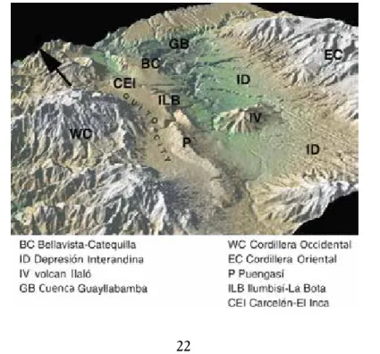
Forming part of this mega fault is a system of blind inverse faults spanning the city of Quito, which can be seen in figure 1, and from south to north are the inver-se faults of: Puengasí (P), Llumbisí-La Bota (ILB), Carcelén-El Inca (CEI) and Bella Vista-Catequilla (BC).

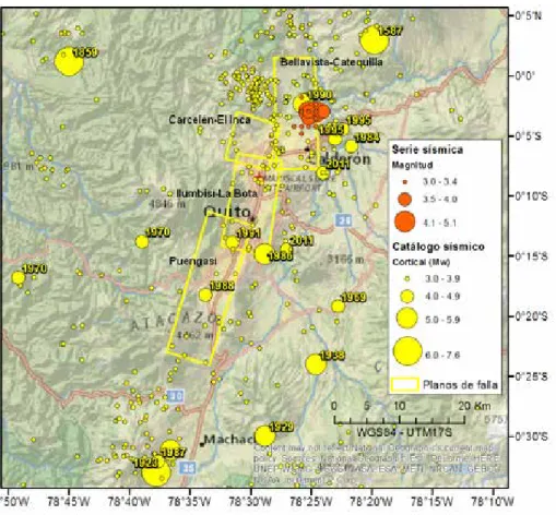
Figure 2 shows a numerical calculation model of possible fault planes that could be generated in the case of earthquakes occuring with a burst length equal to the maxi-mum distance of each of the fault segments. The model assumes that these events are not produced simultaneously (Alvarado et al. 2014; Rivas et al. 2014). The fault planes are shown projected in a horizontal plane.

The largest recorded earthquake associated with the blind faults is that of 1587 which had a magnitude of 6.4, with a shallow focal point (Beuval et al. 2010). This is very worrying as much of the city lies on the same faults (on the slopes of the moun-tains) and hopefully their foundations are well anchored to the ground, because the ver-tical component will be very high, as happened in the earthquake of Christchurch, New Zealand (2011), to cite one of the most recent associated with blind faults under a city.

Figure 1: Quito bounded on the west by the western mountains and east by the fault system: Puengasí (P), Ilumbisí-La Bota (ILB) and crossed by the Inca Carcelén (CEI). (Alvarado et al. 2014).

22

1 Introduction

The constant movement of the Nazca plate situated opposite the American plate, in Ecuador, has given rise to the Carnegie ridge located in the Pacific Ocean, to the subduction trench, and to the mega faults which begin in the Gulf of Guayaquil, pass through Colombia by the Romeral faults and end in Venezuela, in the Boconó faults.

Forming part of this mega fault is a system of blind inverse faults spanning the city of Quito, which can be seen in figure 1, and from south to north are the inver-se faults of: Puengasí (P), Llumbisí-La Bota (ILB), Carcelén-El Inca (CEI) and Bella Vista-Catequilla (BC).

Figure 2 shows a numerical calculation model of possible fault planes that could be generated in the case of earthquakes occuring with a burst length equal to the maxi-mum distance of each of the fault segments. The model assumes that these events are not produced simultaneously (Alvarado et al. 2014; Rivas et al. 2014). The fault planes are shown projected in a horizontal plane.

The largest recorded earthquake associated with the blind faults is that of 1587 which had a magnitude of 6.4, with a shallow focal point (Beuval et al. 2010). This is very worrying as much of the city lies on the same faults (on the slopes of the moun-tains) and hopefully their foundations are well anchored to the ground, because the ver-tical component will be very high, as happened in the earthquake of Christchurch, New Zealand (2011), to cite one of the most recent associated with blind faults under a city.

Figure 1: Quito bounded on the west by the western mountains and east by the fault system: Puengasí (P), Ilumbisí-La Bota (ILB) and crossed by the Inca Carcelén (CEI). (Alvarado et al. 2014).

(3)

Figure 2: Seismicity associated with the blind faults of Quito, excluding that of 1859. Desing spectrums for the central north of quito and seismic analysis of steel structures...

Figure 2: Seismicity associated with the blind faults of Quito, excluding that of 1859.

The Christchurch earthquake of 2011, had a magnitude of 6.2, a deep focal point of 5 km, was associated with an oblique inverse fault with an inclination 700 and the city floor had shear wave speeds that were around 300 m/s2. The maximum recorded

acceleration in the zone of the epicenter was nearly double the maximum

hori-zontal acceleration. (Elwood, 2013; Kam and Pampanin, 2011). This earthquake may give us light as to how to be more careful in the design of structures situated around of the blind inverse faults.

Table 1 indicates the periods of recurrence found for each one of the sectors of Quito’s blind faults, found for different magnitude ranges, using the modified model of Gutenberg and Richter, it can be seen that for earthquakes of the highest magnitude

or equal to 6 and less than the maximum expected magnitude the periods of

recurrence are found between 164 and 290 years. (Rivas et al. 2014)

The Christchurch earthquake of 2011, had a magnitude of 6.2, a deep focal point of 5 km, was associated with an oblique inverse fault with an inclination 700 and the city floor had shear wave speeds that were around 300 m/s2. The maximum recorded acceleration in the zone of the epicenter was 2.2 g nearly double the maximum horizon-tal acceleration. (Elwood, 2013; Kam and Pampanin, 2011). This earthquake may give us light as to how to be more careful in the design of structures situated around of the blind inverse faults.

Table 1 indicates the periods of recurrence found for each one of the sectors of Quito’s blind faults, found for different magnitude ranges, using the modified model of Gutenberg and Richter, it can be seen that for earthquakes of the highest magnitude or equal to 6 and less than the maximum expected magnitude ([6,0 <) the periods of recurrence are found between 164 and 290 years. (Rivas et al. 2014)

(4)

24 Range of

magnitude

Period of recurrence (years)

PUESGASÍ ILB CEI BC Tangahuilla

[5,0 - 5,5) 20 - 35 18 - 30 27 - 39 18 - 31 23 - 34

[5,5 – 6.0) 62 - 87 56 - 75 85 - 130 58 - 78 65 - 97

[6,0 < 164 - 262 179 - 279 169 - 279 179 - 290

Mmax 1224 - 2190 _(Mw6,4) 610 - 981 _(Mw6,2) 549 - 952 _(Mw5,9) 908 - 1630 _(Mw6,3) 579 - 1016 (Mw6,0)

The last row of Table 1, shows the maximum expected magnitude in each segment, found by applying the equations of Leonard (2010) and the period of recurrence is ex-pressed as a time interval; the lower intervals are given in the earthquakes of lower magnitude and the one which has the highest floating population density is Ilumbisí--La Bota with around 500 habitants per hectare, for this reason a seismic microzoning study was carried out for north central Quito since many of their constructions are situated in this fault segment.

2 Microzoning of North Central Quito

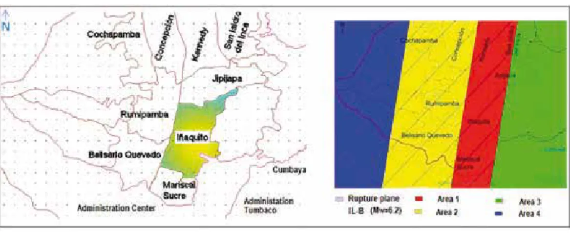
On the left of figure 3 are the north central boroughs and a calculation grid. At each point three spectra associated with an earthquake of magnitude 6.2 were found, which are thought to be located directly in the center of gravity of the fault Ilumbisi-La Bota (ILB); the fault plane can be seen on the right of the figure, with slanted stripes. The spectra were found to match the models of strong movement of Campbell and Bor-zognia (2013), Abrahamson, Silva and Kamai (2013) and Zhao et al. (2006), in short form identified as A & B, A,S & K, and Zhao.

Figure 3: Grid of study and microzoning of North Central Quito

Table 1: Period of recurrence, found using the modified model of Gutenberg and Richter. Range of

magnitude _PUESGASÍ _ILB Period of recurrence (years)_CEI _BC _Tangahuilla

[5,0 - 5,5) 20 - 35 18 - 30 27 - 39 18 - 31 23 - 34

[5,5 – 6.0) 62 - 87 56 - 75 85 - 130 58 - 78 65 - 97

[6,0 < 164 - 262 179 - 279 169 - 279 179 - 290

Mmax 1224 - 2190 _(Mw6,4) 610 - 981 _(Mw6,2) 549 - 952 _(Mw5,9) 908 - 1630 _(Mw6,3) 579 - 1016 (Mw6,0)

The last row of Table 1, shows the maximum expected magnitude in each segment, found by applying the equations of Leonard (2010) and the period of recurrence is ex-pressed as a time interval; the lower intervals are given in the earthquakes of lower magnitude and the one which has the highest floating population density is Ilumbisí--La Bota with around 500 habitants per hectare, for this reason a seismic microzoning study was carried out for north central Quito since many of their constructions are situated in this fault segment.

2 Microzoning of North Central Quito

On the left of figure 3 are the north central boroughs and a calculation grid. At each point three spectra associated with an earthquake of magnitude 6.2 were found, which are thought to be located directly in the center of gravity of the fault Ilumbisi-La Bota (ILB); the fault plane can be seen on the right of the figure, with slanted stripes. The spectra were found to match the models of strong movement of Campbell and Bor-zognia (2013), Abrahamson, Silva and Kamai (2013) and Zhao et al. (2006), in short form identified as A & B, A,S & K, and Zhao.

(5)

The study conducted (Trujillo 2014, Aguiar et al. 2015) obtained four micro zones which are indicated at the right of figure 4. Zone 1 is the most dangerous because it is in the hanging wall and is on the ILB segment. The least dangerous is that found outside the fault plane.

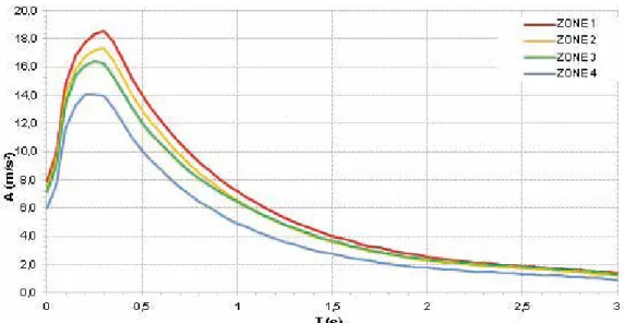
Elastic response spectra were found for a level of reliance of 84% and were obtai-ned by weighing up the following: 35% of the model of C & B; 35% of the model of A, S & K and 30% of the model of Zhao. The spectra found are shown in figure 4.

Figure 4: Elastic response spectra for each earthquake micro zone.

The study conducted (Trujillo 2014, Aguiar et al. 2015) obtained four micro zones which are indicated at the right of figure 4. Zone 1 is the most dangerous because it is in the hanging wall and is on the ILB segment. The least dangerous is that found outside the fault plane.

Elastic response spectra were found for a level of reliance of 84% and were obtai-ned by weighing up the following: 35% of the model of C & B; 35% of the model of A, S & K and 30% of the model of Zhao. The spectra found are shown in figure 4.

Figure 4: Elastic response spectra for each earthquake micro zone.

3 NEC-11 And ERN-12 Response Spectrums

For the area of short periods, less than 0.5 seconds, the ordinates of the spectra associated with the ILB fault are higher than those reported by The Ecuadorian Cons-truction Regulations (Norma Ecuatoriana de la Construcción, NEC-11), or those that are obtained based on site factors found in the earthquake microzoning study of ERN-12 (Aguiar 2013). However, for intermediate periods and larger, they are less than those found with the NEC-11 or ERN-12.

3 NEC-11 And ERN-12 Response Spectrums

For the area of short periods, less than 0.5 seconds, the ordinates of the spectra associated with the ILB fault are higher than those reported by The Ecuadorian Cons-truction Regulations (Norma Ecuatoriana de la Construcción, NEC-11), or those that are obtained based on site factors found in the earthquake microzoning study of ERN-12 (Aguiar 2013). However, for intermediate periods and larger, they are less than those found with the NEC-11 or ERN-12.

(6)

26

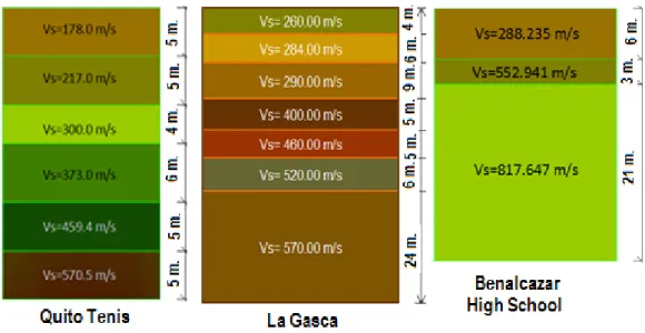
Figure 5: Shear wave velocities in three areas of North Central Quito.

Figure 5 shows the shear wave velocity V_S in three sectors of north central Quito,

which are the old Quito Tenis, which is located in zone 2; La Gasca which can be found in zone 1 and Benalcazar High School which is situated in zone 2, of the microzoning. For these three sites it is subsequently considered that they all have steel structures from one to nine storeys.

The site factors of the NEC-11 are at the macro level, valid and applicable to all of Ecuador. However, those of ERN-12 correspond to the land type of the city of Quito but were calibrated to use the same equations of NEC-11.With this in mind, table 2 presents the site factors for the three sites of figure 5; furthermore, indicating in which zone they are in accordance with figure 3.

Table 2: Site factors for the sites of North Central Quito following NEC-11 and ERN-12 Site

Factors

“Quito Tenis” “La Gasca” “Benalcazar” High school

NEC11 ERN12 ILB NEC11 ERN12 ILB NEC11 ERN12 ILB

Fa 1.20 1.155 Zone2 1.20 1.055 Zone1 1.20 1.255 Zone2 Fd 1.40 0.575 1.40 1.505 1.30 1.105 Fs 1.50 1.790 1.50 0.740 1.30 1.225

The spectra obtained with the data in table 2 is shown in figure 6, where it is clear that, for all cases, in the area of short periods, the spectral ordinates that are generated from the earthquake of 6.2 magnitude in fault ILB is considerably higher than those found with NEC-11 or ERN-12; this may lead one to think that it is safer to calculate

(7)

all of the structures located in north central Quito with the spectrum of ILB, which is actually false, as you will see later.

Figure 6: Spectra found with NEC-11, ERN-12 and ILB for three sectors of north central Quito.

4 Seismic analysis of steel structures.

It was deemed that all of the frames of the steel structures of 1 to 9 storeys have three bays each, with 7.315 m. lights, and mezzanine heights of 3.81 m., equal in all the storeys; the uniform load in each storey is 3.269 T/m. Also indicated are the sections of the “I” steel profiles; it is clear that the exterior columns have a larger transversal section than the interior columns.

Figure 7: Geometry and loads of the buidings of a 4 storey and a 2 storey.

3 @ 7.315 m = 21.945 4 @ 3 .8 10 m = 1 5. 240 3 @ 7.315 m = 21.945 2 @ 3. 81 0 m = 7. 62 0 3.269 T/m W14X 193 W14X 193 W30X99 W30X99 W30X99 W30X99 W30X99 W30X99 W30X 173 W30X 173 3.269 T/m W30X99 W30X99 W30X99 W30X99 W27X94 W30X99 W30X99 W27X94 W27X94 W27X94 W27X94 W27X94 3.269 T/m 3.269 T/m 3.269 T/m 3.269 T/m W14X 193 W30X 173 W30X 173 W14X 159 W27X 146 W14X 193 W27X 146 W14X 159

Figure 7 serves to explain the sections used, for all of the structures analysed and presented in table 3. The 2 storey structure has columns with W14X193 profiles in the exterior part and W30X173; these sections remain in all of the analysed 1 to 9 storey structures. Therefore, they can be seen in the first two storeys of the four storey frame whilst in the third and fourth storeys W14X159 and W27X146 profiles are shown. For those of six storeys the structures remain the same for the first four storeys and for the fifth and sixth appear as W14X109 y W24X104 profiles. A similar pattern is followed for beams.

(8)

28

On the other hand, working with symmetrical sections and uniform sections, the moment curvature diagram, in the initial node, is equal to that of the center of light and the final node; furthermore, these values are equal if there is traction on the lower fibers or the upper fibers, in the case of beams; and it is a similar thing for columns.

Therefore, in table 3 the yield moment indicated My and its associated curvature y

and the moment formed by the plastic ball-and-socket Mu and its associated curvature

Øu need no further explanation. In the case of columns, the third column indicates the

movement of the axial load.

Table 3: Sections, the moment curvature diagram and axial stiffness of columns Floors Section P (T.) My (Tm.) Mu (Tm.) _y (1/m) _u (1/m) EA (T.) 1 & 2 W14X193 927.12 147.18 176.62 0.00702 0.07718 769546.85 1 & 2 W30X173 832.45 251.66 301.99 0.00350 0.03848 690966.36 3 & 4 W14X159 762.26 118.99 142.79 0.00716 0.07881 632708.41 3 & 4 W27X146 703.50 192.37 230.85 0.00389 0.04277 583934.32 5 & 6 W14X109 522.32 79.60 95.52 0.00734 0.08079 433547.52 5 & 6 W24X104 499.47 119.82 143.78 0.00442 0.04864 414579.82 7 & 8 W14X99 474.99 71.72 86.07 0.00739 0.08132 394257.28 9 W14X82 391.74 57.63 69.15 0.00748 0.08232 325160.62

Table 4: Sections, the momentum curvature diagram and axial stiffness of beams

Floors Section My (Tm.) (Tm.)Mu (1/m)y (1/m)u (T.)EA 1 & 2 W30X99 129.35 155.22 0.00371 0.04080 394257.28 3 & 4 W27X94 115.26 138.31 0.00403 0.04436 375289.57 5 & 6 W24X76 82.92 99.50 0.00452 0.04969 303483.26 7 & 8 W24X62 63.43 76.12 0.00468 0.05150 246580.15 9 W21X48 44.36 53.23 0.00529 0.05821 191031.88

(9)

Figure 8: Bilinear model of the moment curvature diagram.

Øy Øu EI EI Øy Øu My Mu e e p p Y U Y U M Ø EI EI Mu My

Figure 8 shows the bilinear model of the moment curvature diagram that was worked with. For the calculation of the elastic stiffness Ele it was deemed that a

modu-lus of elasticity of steel was equal to 21000000T/m2_{. The yield moment was obtained}

with the following equation.

M_Y = Z_X fy (1)

Where Z_X is the plastic section modulus that is equal to the static moment of the

areas of tension and compression in respect to its neutral axis (Zx = ∫ y dA); y is the yield stress of the steel, the steel used was ASTM A36 with.

With the elastic rigidity Ele; and the yield moment MY the curvature of yield is

determined ( = My/Ele). On the other hand, the rigidity in the inelastic range Elp has the following expression.

Elp = a Ele (2)

It is calculated with the value a = 0,02, which is a conservative value, much as

Mu = 1.2 My, which was the way that the plastic moment was obtained, is also

consi-dered a conservative value. Finally, the curvature u was obtained from the bilinear model shown in figure 8, with the following equation.

Figure 8: Bilinear model of the moment curvature diagram.

Øy Øu EI EI Øy Øu My Mu e e p p Y U Y U M Ø EI EI Mu My

Figure 8 shows the bilinear model of the moment curvature diagram that was worked with. For the calculation of the elastic stiffness Ele it was deemed that a

modu-lus of elasticity of steel was equal to 21000000T/m2_{. The yield moment was obtained}

with the following equation.

M_Y = Z_X fy (1)

Where Z_X is the plastic section modulus that is equal to the static moment of the

areas of tension and compression in respect to its neutral axis (Zx = ∫ y dA); y is the

yield stress of the steel, the steel used was ASTM A36 with.

With the elastic rigidity Ele; and the yield moment MY the curvature of yield is

determined ( = My/Ele). On the other hand, the rigidity in the inelastic range Elp has the following expression.

Elp = a Ele (2)

It is calculated with the value a = 0,02, which is a conservative value, much as

Mu = 1.2 My, which was the way that the plastic moment was obtained, is also

consi-dered a conservative value. Finally, the curvature  u was obtained from the bilinear model shown in figure 8, with the following equation.

(3) All of the variables shown in equation (3) have been defined.

(10)

5 Capacity spectrum method

The resistant seismic capacity curve that relates to the base shear V with a late-ral displacement at the top of the structure Dt is found, by means of non-lineal sta-tic analysis working with the concentrated plassta-ticity model of Giberson (1969) and applying the lateral load increments in each storey, proportional to the first mode of vibration, employing the following equation. (ATC-40, 1996)

5 Capacity spectrum method

(4) Where the subindex i makes reference to the storey i; with this noted F is the late-ral force; w the weight,  is the first mode of vibration and Vo is the base shear that is imposed on each one of the load cycles.

In Aguiar et al. (2015) the theoretical framework of resistant seismic capacity cur-ves V – Dt is well detailed, as well as the way that the capacity spectrum is obtained

Sa – Sd, by means of the following equations:

(5)

(6) Where Dti Vi are the coordinates of a point on the resistant seismic capacity curve for which the displacement and spectral acceleration are determined Sdi; Sai; Mt is the

total mass of the tructure; a₁ is the modal mass ratio of the first mode; FP₁ is the modal

participation factor of the first mode.

(7)

(8) The variables still not indicated are: M is the mass matrix; J is the vector of inci-dence of land movement with the lateral coordinates of the structure; in two dimensions

J is a unitary vector. It is highlighted that the modal participation factor is obtained in

30

5 Capacity spectrum method

(5)

total mass of the tructure; a1 is the modal mass ratio of the first mode; FP1 is the modal

(7)

(5)

5 Capacity spectrum method

(5)

(7)

5 Capacity spectrum method

(5)

(7)

5 Capacity spectrum method

(5)

(7)

(11)

an absolute value. On the other hand, using the pseudo spectrum definition, the sought for spectra are found in the format Sd – Sa. Being Sa the spectral acceleration and Sd the spectral displacement. Finally, the Capacity Spectrum Method is applied which is very well detailed in Aguiar et al. (2015). However, it is indicated that the damping factor, for when the structure works in the non-linear range, is obtained employing a bilinear hysteresis model with the equation proposed by Jennings (1968)

(9)

Where E_D the energy is dissipated per cycle in hysteretic behavior; E_S is the strain

energy stored elastically; a is the relationship between the post yield stiffness with

respect to the elastic stiffness of the bilinear model; μ is the ductility demand.

The ATC-40 considering the imperfections of the hysteresis curves, in the sense that they are not straight as they were expected to be in the bilinear model without

curves, introduces a correction factor K in accordance with the standard of the structural

de-sign. Such that the effective viscous absorption is:

(10) Where 𝜉𝜉 is the inherent equivalent viscous damping of the structure. Once the damping factor is obtained 𝜉𝜉 e  the respective inelastic spectrum is found by dividing the ordinates of the elastic spectrum by B.

(11) The interception of the capacity spectrum of the structure with the seismic de-mand spectrum determines the performance point, it should comply with the ductility demand by which the effective damping factor value is obtained and, subsequently, factor B is approximately equal to the ductility demand of the performance point, if not so, the calculation is repeated.

When the structure works in the elastic range, the interactive calculation is not made; in this case the performance point as well as the section point of the demand and capacity spectrum are obtained directly. But when the linear range is exceeded, the performance point is obtained interactively; in this case, in the graphs presented in the following section, the spectrum of initial seismic demand (elastic range) is shown and final with/ending whatever verifies the equality of ductilities, they are the graphs which are divided by B. Intermediate positions of calculation are not indicated.

(9)

energy stored elastically; a is the relationship between the post yield stiffness with respect to the elastic stiffness of the bilinear model; μ is the ductility demand.

(9)

(10) Where 𝜉 is the inherent equivalent viscous damping of the structure. Once the damping factor is obtained 𝜉 e  the respective inelastic spectrum is found by dividing the ordinates of the elastic spectrum by B.

(9)

(12)

32

6 Performance results point

Figure 8 shows 8 graphs; those in the first row correspond to the structures with 1 to 3 storeys; the second, to those with 4 to 6 storeys and the last three to those of 7 to 9 storeys. These graphs show the performance point of the structures situated in old Quito Tenis, i.e. using the spectrum found on the left in figure 6.

In figure 8 it is appreciated that the structures with 1 to 5 storeys work in the elastic range and, for these, the largest displacement of the point of demand is found with the spectrum associated with the fault Ilumbisi-La Bota (ILB). In contrast, for the structures with 6 to 9 storeys the largest displacements are found with the spectrum of the NEC-11.

(13)

7 Storey displacement

Presented in the previous section, was the performance point of the structures with 1 to 9 storeys, situated in the old Quito Tenis; the structures situated at the other two sites have similar behavior. Therefore, a presentation of these is not included and in its place is a presentation of the lateral displacements in each storey that are obtai-ned from the performance point considering that the structure works in the first mode of vibration.

It is noted that the displacement corresponding with the performance point S_d is

not the maximum displacement of the structure, it is a displacement associated with a

system of one degree of freedom, in order to position the displacement at the top D_y the

equation (6) is used, i.e. S_d is multiplied by the factor of modal participation FP at the

performance point. Finally, the displacements in each storey are found multiplying D_t

by the first mode of vibration that was normalized to the unit at the top.

These results are shown for the structures situated in La Gasca, in the same for-mat as figure 8, i.e. the graphs of the first row correspond to the lateral displacements of the structures with 1 to 3 storeys; in the second row come the lateral displacements of the structures with 4 to 6 storeys and the third row corresponds to the structures with 7 to 9 storeys.

In the structures with 1 to 6 storeys, the largest lateral displacements arise from the spectrum of Ilumbisí (ILB). For the structures with 7 to 9 storeys the maximum displacements are found applying the spectrum of the NEC-11. It is a result similar to that obtained in the previous section when working with the performance point.

(14)

34

Figure 9: Storey Displacement with NEC11, ERN12 and ILB Spectrums “La Gasca”

8 Interstorey drifts

Another indicator of structural damage is the interstorey drift, figure 10 shows the interstorey drift found in the steel structures with 1 to 9 storeys, assuming that the buildings are located in the Benalcazar High school. For the structures with 1 to 5 storeys the largest values are found with the spectrum of Ilumbisi.

In the structures of 6 storeys the largest interstorey drifts are found with the spectrum ERN-12, this is the only case of those studied in which the largest seismic demands are found with this spectrum. In the structures with 7 to 9 storeys, the máxi-mum interstorey drifts are found with the spectrum of the NEC-11.

Table 5 shows the fundamental periods of vibration of each one of the steel struc-tures. Furthermore, as indicated, the structures with 1 to 5 storeys work in the elastic range, and those with 6 to 9 storeys had a small incursion in the inelastic range so that the vibration period in the performance point was practically the same as in the elastic range. The above is confirmed by the values of B (equation 11) seen/used with those that were obtained by the performance point of the structures situated in the old Quito Tenis. These values are shown in table 6

(15)

Table 5: Elastic periods in each steel structure

Floor 1 2 3 4 5 6 7 8 9

T(s) 0.09 0.18 0.27 0.37 0.48 0.59 0.72 0.86 1.01

Figure 10: Interstorey drift with NEC11, ERN12 and ILB Spectrums “Benalcazar” High school

Table 6: Values of Bwith which the elastic spectrum is reduced, for the structures situated

in the old Quito Tenis.

Floor 1 2 3 4 5 6 7 8 9

NEC 1 1 1 1 1 1.04 1.18 1.29 1.41

ERN 1 1 1 1 1 1 1 1 1

(16)

36

9 Comments and conclusions

The periods of recurrence that are expected in each of the segments of the blind in-verse faults of Quito have been presented, for different ranges of magnitude, employing Gutenberg and Richter’s model, modified and truncated. Subsequently, the microzo-ning found in North Central Quito is presented in the face of a probable earthquake of 6.2 magnitude, in the fault of Ilumbisí-La Bota.

For North Central Quito there are three spectra and they are those of the Ecuado-rian Construction Regulations (Norma EcuatoEcuado-riana de la Construcción NEC-11); that found in the study of seismic microzoning, ERN-12 and that obtained from an earth-quake in the fault Ilumbisi-La Bota which has been referred to as ILB. The big ques-tion is to find out with which spectrum, of the three, a structure should be designed. To answer the question, a seismic analysis was carried out of nine steel structures of 1 to 9 storeys, using the Capacity Spectrum Method and assuming that they are on three different sites in North Central Quito. The performance points found were obtained with the Capacity Spectrum Method/MEC, as well as the lateral displacements and the interstorey drifts, for the 27 cases of the study.

In order not to make the presentation too long, the performance point found in the Capacity Spectrum Method/MEC for the structures situated in the old Quito Tenis was presented; the maximum lateral displacements found in the structures of La Gasca and the interstorey drifts found in the structures situated in Colegio Benalcazar were also presented. It is noted that the lateral displacements and the interstorey drifts were obtained from the performance point.

From the study carried out, it can be concluded that for structures with periods less than 0.5 seconds the spectrum ILB should be used. In the study, these structures have 1 to 5 storeys. For structures with periods more than 0.5 seconds it cannot be said categorically that the spectrum of NEC-11 should be used because there was a case in which the largest responses were found with the spectrum ERN-12.

Considering that programs are currently available that facilitate seismic analysis, it is recommended that any structures that are going to be projected in North Central Quito be analyzed with the three spectra: NEC-11, ERN-12, and ILB.

10 References

Abrahamson N., Silva W., Kamai R. (2013), Update of the AS08 Ground-Motion Prediction Equa-tions Based on the NGA-West2 Data Set. Pacific Earthquake Engineering Research Center, PEER, 143 p.

Abrahamson N., Silva W., Kamai R., (2014), “Summary of the ASK14 ground motion relation for active cristal regions”, Earthquake Spectra, 30 (3), 1025-1055.

Aguiar Roberto, (2013), Microzonificación sísmica de Quito, Centro de Investigaciones Científi-cas. Universidad de Fuerzas Armadas, ESPE, Primera Edición, 212 p.

(17)

Aguiar Roberto, (2010), “Peligrosidad sísmica del Ecuador y descripción de los puentes construi-dos sobre el estuario del río Esmeraldas con aisladores de base FPS’, Revista Internacional de Ingeniería de Estructuras, 15 (1), 85-118.

Aguiar Roberto, Mora David, Morales Enrique, (2015), “Peligrosidad sísmica de Quito y el Mé-todo del Espectro de Capacidad con CEINCI-LAB”, Revista Internacional de Ingeniería de Es-tructuras, 20 (1), 1-39.

Aguiar Roberto, (1998), Acciones para el diseño sísmico de estructuras, Centro Internacional de Métodos Numéricos, CIMNE. Monografías de Ingeniería Sísmica, IS-30, 122 p.

Alvarado A., Audin L., Nocquet M., Lagreulet S., Segovia M., Font Y., Lamarque G., Yepes H., Mothes P., Rolandone F., Jarrín P., and Quidelleur X., (2014), “Active tectonics in Quito, Ecuador, assessed by geomorpholigical studies, GPS data, and crustal seismicity”, Tectonics, AGUPLICA-TIONS, 17 p., Article online.

Bozorgnia, Y., Abrahamson, N., Al Atick, L., Ancheta, T., Atkinson, G., Baker, J., Rezaeian. (2014). NGA-West2 Research Project. Pacific Earthquake Engineering Research Center, Univer-sity of California, Berkeley, CA.

Beauval C., Yepes H., Bakun W., Egred J., Alvarado A., and Singaucho C., (2010), “Locations and magnitudes of historical earthquakes in the Sierra of Ecuador (1586- 1996), Geophys. Journal International, 181, 1613-1633.

Campbell K., Bozorgnia Y., (2013), NGA-West2 Campbell-Bozorgnia ground motion model for the horizontal components of PGA, PGV and 5%-Damped elastic Pseudo-Acceleration response spectra for periods ranging fro 0.01 to 10 sec, Pacific Earthquake Engineering Research Center, PEER, 75 p.

Elwood, K. (2013). Performance of concrete buildings in the 22 February 2011 Christchurch earthquake and implications for Canadian codes. Canadian Journal of Civil Engineering 40, 759-776.

ERN-2012, Microzonificación sísmica del distrito metropolitano de Quito: Estudio de la amenaza sísmica a nivel local. Programa para la reducción de riesgos urbanos. Distrito Metropolitano de Quito.

Leonard M., (2010), “Earthquake fault scaling: Self consistent relating of rupture length width, average displacement, and moment release”, Bulletin of the Seismological Society of America, 100 (SA), 1971-1988.

Kam, W.Y., Pampanin, S. (2011). The seismic performance of RC buildings in the 22 February 2011 Christchurch earthquake. Structural Concrete 12 (4), 223-233.

NEC-11 (2014) Norma Ecuatoriana de la Construcción, Ministerio de Desarrollo Urbano y Vi-vienda, MIDUVI.

Rivas A., Aguiar R., Benito M. B., Gaspar J., Parra H., (2014), Determinación del período de recurrencia y magnitud máxima para el control de las estructuras en el rango elástico ante un sismo asociado a las fallas inversas de Quito, Revista Internacional de Ingeniería de Estructu-ras, 19 (2), 201-217.

Trujillo Santiago (2014), Espectro de Control para el Centro Norte de Quito, Tesis de Grado para obtener título de Ing. Civil. Universidad de Fuerzas Armadas ESPE, 95 p. Quito.

(18)

38

Espectros de diseño para el centro norte de quito y análisis

sísmico de estructuras de acero por el método del espectro de

capacidad

RESUMEN

La ciudad de Quito se halla sobre fallas geológicas, que no tienen afloramiento super-ficial pero están en movimiento con una velocidad de 2 a 4 mm., por año. El último sismo fuerte, asociado a estas fallas inversas, se registró en 1587 y tuvo una magnitud de 6.4; de tal manera que ha transcurrido más de 400 años con lo que la acumulación de energía es muy grande y la probabilidad de ocurrencia de un sismo es muy alta por lo que en este artículo se presenta en primer lugar los períodos de recurrencia de estas fallas; luego una microzonificación del Centro Norte de la ciudad y los espectros de respuesta elásticos para 5% de amortiguamiento asociados al segmento de falla Ilum-bisí-La Bota, ILB. Posteriormente se analizan 9 estructuras de acero de 1 a 9 pisos, que se suponen están situadas en 3 diferentes suelos del Centro Norte de Quito y son los siguientes barrios: antiguo Quito Tenis; La Gasca; El Colegio Benalcazar. Se halla la respuesta sísmica, empleando el Método del Espectro de Capacidad MEC, ante tres espectros y son el prescrito en la Norma Ecuatoriana de la Construcción NEC-11; el recomendado en el estudio de microzonificación sísmica de Quito ERN-12 y los hallados en la micro zonificación sísmica asociados a la falla ILB. Para las estructuras ubicadas en el antiguo Quito Tenis se presenta el punto de desempeño hallado en el MEC; para las que se hallan en La Gasca se indican los desplazamientos laterales máximos en cada piso y para las estructuras ubicadas en el Colegio Benalcazar se presenta las derivas máximas de piso. Se destaca que a partir del punto de desem-peño se hallan los desplazamientos laterales y derivas de piso, de tal manera que las conclusiones que se hallan en este estudio sobre con que espectro se tienen las máxi-mas respuestas se pueden inferir con cualquiera de los tres parámetros estructurales.

Comentarios y conclusiones

Se ha presentado los períodos de recurrencia, que se esperan en cada uno de los segmentos de las fallas ciegas inversas de Quito, para diferentes rangos de magnitud, empleando el modelo de Gutenberg y Richter modificado y truncado. Posteriormente se presenta la micro zonificación encontrada en el Centro Norte de Quito ante un probable sismo de magnitud 6.2, en la falla de Ilumbisí-La Bota.

Para el Centro Norte de Quito se tienen tres espectros y son el de la Norma Ecuato-riana de la Construcción NEC-11; el hallado en el estudio de micro zonificación sísmica ERN-12 y el obtenido a partir de un sismo en la falla Ilumbisi-La Bota que se ha deno-minado ILB. La gran interrogante que se tiene es saber con que espectro, de los tres, se debe diseñar una estructura. Para contestar esta pregunta se realizó el análisis sísmico de 9 estructuras de 1 a 9 pisos de acero, por el Método del Espectro de Capacidad supo-niendo que están situadas en tres sitios diferentes del Centro Norte y se obtuvieron los

(19)

puntos de desempeño hallados con el MEC, los desplazamientos laterales y las derivas de piso, para los 27 casos de estudio.

Para no alargar la presentación de resultados se presentó el punto de desempeño hallado en el MEC para las estructuras situadas en el antiguo Quito Tenis; los despla-zamientos laterales máximos encontrados en las estructuras ubicadas en La Gasca y las derivas de piso halladas en las estructuras situadas en el Colegio Benalcazar. Se destaca que a partir del punto de desempeño se obtienen los desplazamientos laterales y las derivas de piso.

Del estudio realizado se concluye que para estructuras con períodos menores a 0.5 seg., se debe utilizar el espectro ILB. En el estudio estas estructuras son de 1 a 5 pisos. Para estructuras con períodos mayores a 0.5 seg., no se puede decir en forma categórica que se debe utilizar el espectro del NEC-11 porque hubo un caso en que las mayores respuestas se hallaron con el espectro ERN-12.

Considerando que actualmente se disponen de programas, que facilitan el análisis sísmico, se recomienda que las estructuras que se van a proyectar en el Centro Norte de Quito sean analizadas con los tres espectros: NEC-11, ERN-12, ILB.