www.scielo.br/aabc
Stoichiometry-based estimates of ferric iron in calcic, sodic-calcic
and sodic amphiboles: A comparison of various methods
GUILHERME A.R. GUALDA∗ and SILVIO R.F. VLACH
Departamento de Mineralogia e Geotectônica, Instituto de Geociências, Universidade de São Paulo Rua do Lago, 562, Cidade Universitária, 05508-080, São Paulo, SP, Brasil
Manuscript received on July 9, 2004; accepted for publication on January 12, 2005; presented byAntonio C. Rocha-Campos
ABSTRACT
An important drawback of the electron microprobe is its inability to quantify Fe3+/Fe2+ratios in routine work. Although these ratios can be calculated, there is no unique criterion that can be applied to all amphiboles.
Using a large data set of calcic, sodic-calcic, and sodic amphibole analysis from A-type granites and syenites from southern Brazil, we assess the choices made by the method of Schumacher (1997, Canadian Mineralogist, 35: 238-246), which uses the average between selected maximum and minimum estimates. Maximum estimates selected most frequently are: 13 cations excluding Ca, Na, and K (13eCNK – 66%); sum of Si and Al equal to 8 (8SiAl – 17%); 15 cations excluding K (15eK – 8%). These selections are appropriate based on crystallochemical considerations. Minimum estimates are mostly all iron as Fe2+(allFe2 – 71%), and
are clearly inadequate. Hence, maximum estimates should better approximate the actual values.
To test this, complete analyses were selected from the literature, and calculated and measured values were compared. 13eCNK and maximum estimates are precise and accurate (concordance correlation coefficient – rc≈0.85). As expected, averages yield poor estimates (rc= 0.56).
We recommend, thus, that maximum estimates be used for calcic, sodic-calcic, and sodic amphiboles.
Key words:amphiboles, stoichiometry, ferric iron, EPMA.
INTRODUCTION
The electron microprobe analyzer (EPMA) has be-come the standard instrument for the chemical anal-ysis of minerals. It allows for very good spatial res-olution and reasonable detection limits for the vast majority of the materials of interest to Earth scien-tists. However, one of the most crucial problems is its inability, at least in routine work, to
discrimi-Correspondence to: Guilherme Augusto Rosa Gualda E-mail: [email protected]
*Present address: Department of the Geophysical Sciences, The University of Chicago, Chicago, IL 60637, U.S.A.
nate between different oxidation states of chemical elements.
Due to the mineralogical and petrologic rele-vance of such determinations, particularly the im-portance of the Fe3+/Fe2+ratio as an indicator of in-tensive and exin-tensive parameters of crystallization, several techniques have been applied in order to es-timate them.
time-consuming and its applicability may be ques-tioned in most cases due to the presence of inclusions and chemical zoning.
Recently, there has been an effort to develop microanalytical methods sensitive to these vari-ations. Yet, although some techniques have been successful, none of them became widespread until now. Some of them depend on the availability of very specialized equipment (e.g. microXANES – cf. Sutton et al. 1993, Delaney et al. 1996), while other potential methods employing the EPMA (e.g. flank method – cf. Enders et al. 2000, and ref-erences therein) require much more care and time than it is usually possible in routine work.
In this sense, estimates based on stoichio-metric considerations are still the best choice for or-dinary analyses. For several minerals with relatively simple structures and in which only one element is present in two valence states (e.g. pyroxene, garnet), these calculations are sufficiently good, provided the analyses are of high quality (Droop 1987).
Amphiboles, however, have long challenged researchers and, consequently, an extensive litera-ture has developed on the subject (e.g. Papike et al. 1974, Robinson et al. 1982, Hawthorne 1983, Schumacher 1991, 1997).
The presence of vacancies in the A-site and the potential substitution of (OH)–, F–and Cl– for
O2–prevent the determination of a unique
crystallo-chemical criterion on which to base the calculations. It has been recognized that different criteria may ap-ply to different amphibole groups (cf. Robinson et al. 1982). Accordingly, the IMA has recently pro-posed a method to choose from among the various criteria (Leake et al. 1997, Schumacher 1997) that is very similar to that of Holland and Blundy (1994). However, some recent studies suggest this method may yield unsatisfactory results (Enders et al. 2000, Martins 2001).
In this paper, we use a large dataset of cal-cic, sodic-calcal-cic, and sodic amphibole compositions obtained along the study of the mineralogy of the Graciosa A-type Granites, southern Brazil (Gualda 2001), to critically evaluate the choices made by the
method of Schumacher (1997). Also, we compare the results obtained from published complete anal-yses with the calculated Fe3+and Fe2+contents in
order to assess the quality of the estimates. Finally, we propose that a variation of the method of Schu-macher (1997) be used for calcic, sodic-calcic, and sodic amphiboles.
BACKGROUND
Methods for the calculation of Fe2+ and Fe3+ con-tents from total Fe are based on an assumption of electroneutrality (Hawthorne 1983). In fact, the same approach may be applied for any other el-ement, provided it is the only one present in two different oxidation states. The solution consists in distributing total Fe contents in a way that the pos-itive charges equal the negative ones. However, the analytical determination of the number of negative charges is seldom viable. Although the measure-ment of oxygen concentrations with the EPMA is possible in some cases, it is usually problematic, at least in routine work with silicates.
If a group of cations is restricted to one or more crystallographic sites, it becomes possible to con-vert the measured cation proportions into absolute cations per unit formula. This is done by normaliz-ing all cations so that the sum of the selected group equals the expected value (for example, in pyrox-enes, the sum of all cations should be normalized to 4). The positive charges can then be balanced to the expected number of negative charges in the same unit cell (in the case of pyroxenes, total Fe is split into Fe3+ and Fe2+ so that the sum of positive
charges equals twelve, equivalent to the 6 oxygen anions). This general formalism was presented by Droop (1987), and is an exact solution to the iterative method of Papike et al. (1974).
In the case of the amphiboles, however, the presence of vacancies in the A site precludes the normalization to 16 total cations. Likewise, the po-tential presence of Al in both T and C sites, of Fe2+,
any of these partial sums to normalize the cationic contents.
Although no single criterion is suitable for all possible amphibole compositions (Hawthorne 1983), it has been argued that each criterion may be applicable to some specific amphibole groups (Robinson et al. 1982), in which case, site occupancy considerations show that corrected analyses tend to be more satisfactory than uncorrected ones (Schu-macher 1991). The distribution of elements present among multiple sites is not reliable, though. Con-sequently, the challenge is to choose, from among the possible criteria, the best suited for a given am-phibole analysis. The IMA recently recommended the adoption of a method to make such a decision (Schumacher 1997).
Each of the nine crystallochemical criteria considered by Schumacher (1997) leads to a differ-ent estimate of Fe3+. Four of them result in
minimum Fe3+estimates:
(a) 8 Si cations (8Si);
(b) 16 total cations (16Cat);
(c) 15 total cations excluding Na and K (15eNK);
(d) all Fe as bivalent (allFe2);
whereas five result in maximum estimates:
(e) 8 (Si+Al) cations (8SiAl);
(f) 15 total cations excluding K (15eK);
(g) 13 total cations excluding Ca, Na and K (13eCNK);
(h) all Fe as trivalent (allFe3);
(i) all tri- and tetravalent cations in the M2 sites (10SFe3).
The actual value of Fe3+ should lie between
the larger Fe3+value among the minimum estimates
and the smaller one among the maximum es-timates. Schumacher (1997) proposes that the final Fe3+ result be calculated based on the average
be-tween these two values. It is pointed out, however, that this last recommendation is a rather arbitrary one, because the actual values may lie anywhere between the two estimates.
ANALYTICAL PROCEDURES
Amphibole analysis (wavelength-dispersive spec-trometry, WDS) were obtained at the Instituto de Geociências, Universidade de São Paulo, using stan-dard carbon-coated thin sections on a JEOL-8600S EPMA with five WD spectrometers, a Noran EDS (energy-dispersive spectrometry) detector, and a Voyager (v. 3.6.1) automation and data reduction system.
A total of 20 samples from alkaline and other 19 from aluminous A-type granite associations cov-ering the observed petrographic variation within the Graciosa granites and syenites were selected for this work.
Analytical conditions were 15 kV, 20 nA, and 5µm for accelerating voltage, current, and beam di-ameter, respectively. Si, Ti, Al, Fe, Mn, Mg, Zn, Ca, Na, K, Cl, and F Ka line intensities were quantified along core to rim traverses and/or over areas with contrasted patterns as revealed in transmitted light or back-scattered electron compositional images. Zr (Lα line) contents were below detection limits (ca.
400 ppm) in most analysis. Total counting times were between 20s (major elements) and up to 80s (minor elements, < 1wt.%), equally distributed for peak and background measurements.
Analytical standards included both natural and synthetic compounds: wollastonite (Si, Ca), Are-nal hornblende (Al), synth rutile (Ti), Mn-olivine (Fe, Mn), diopside (Mg), zircon (Zr), Amelia Al-bite (Na), Asbestos microcline (K), synth Cl-apatite (Cl), fluorite/F-apatite (F), synth ZnO (Zn). Ele-mental calibrations were checked against the Arenal and Kakanui hornblende standards in all runs. The PROZA scheme (e.g. Bastin et al. 1984) was used for matrix corrections and data reduction.
THE AMPHIBOLES OF THE GRACIOSA A-TYPE GRANITES
miner-alogical evolution of the Graciosa A-type Granites, which crop out in the Serra do Mar Granitic Province, Southern Brazil (Gualda 2001).
The studied amphiboles show a broad range of compositions, varying from calcic to sodic-calcic to sodic (Figure 1). Calcic amphiboles are present in metaluminous to slightly peraluminous granites that formaluminousA-type associations (Vlach et al. 1990, King et al. 1997). Calcic, sodic-calcic, and sodic amphiboles are present in metaluminous to peralkaline varieties that composealkalineA-type associations (Lameyre and Bowden 1982; for de-tails, see Gualda 2001).
0.0 0.5 1.0 1.5 2.0
0.0 0.5 1.0 1.5 2.0
0.0 0.5 1.0 1.5 2.0
0.0 0.5 1.0 1.5 2.0
[Ca+Na]B Sodic-calcic Sodic Calcic Magnesium-iron-manganese-lithium Na B
Fig. 1 – NaBversus [Ca+Na]Bclassification plot (after Leake et
al. 1997) showing the array variation from calcic to sodic-calcic, and sodic among the amphiboles of the Graciosa A-type Granites, southern Brazil. Calculated on the basis of 23O anions. Fe2+and Fe3+corrected using the method of Schumacher (1997).
Both the presence of widespread chemical zoning patterns and, in many samples, the post-magmatic replacement of sodic-calcic amphibole by sodic varieties prevented the determination of Fe3+/ Fe2+ratios from concentrates. The existence
of a whole range of calcic to sodic amphibole com-positions in our dataset makes it possible to criti-cally assess the adequacy of the method proposed by Schumacher (1997).
The chosen approach was to consider the crys-tallochemical criteria selected by the method (i.e. which minimum and maximum estimates were se-lected, denoted hereafter as minimum and maxi-mum estimates, respectively), which is possible
us-ing the program MINCAL developed by us. Figures 2 and 3 summarize the results. Figure 2 shows the relative frequencies with which each crys-tallochemical criterion was selected by the method, while Figure 3 details the relative frequencies of se-lection of each possible combination of minimum and maximum estimates, for the different amphibole groups from the Graciosa granites and syenites.
0.71 0.17 0.00 0.66 0.26 0.08 0.01 0.00 0.12 0.0 0.2 0.4 0.6 0.8 all Fe2 8Si 15eNK 16Cat 13eCNK 8SiAl 15eK 10SFe3 all Fe3 0.71 0.17 0.00 0.66 0.26 0.08 0.01 0.00 0.12 0.0 0.2 0.4 0.6 0.8 Relative frequency all Fe2 8Si 15eNK 16Cat 13eCNK 8SiAl 15eK 10SFe3 all Fe3 3+
Minimum Fe Maximum Fe3+
Fig. 2 – Histogram of the relative frequencies with which the crys-tallochemical criteria were selected by the method of Schumacher (1997), for the amphiboles of the Graciosa A-type Granites.
MINIMUM Fe3+ESTIMATES
Among the minimum Fe3+estimates, 16Cat was
se-lected only once in the whole set, and hence, there is no need to discuss its applicability. Meanwhile,all
Fe2, 8Si and 15eNK were chosen a significant num-ber of times. TheallFe2 estimates, selected on 71% of the times, are too unrealistic, as there is abundant evidence that Fe3+is present in calcic, sodic-calcic,
and sodic amphiboles (e.g. Hawthorne 1983, Deer et al. 1997, Enders et al. 2000).
Similarly, Al is present in tetrahedral coor-dination in almost every amphibole, with the possi-ble exception of compositions very close to Al-free end-members (Robinson et al. 1982), especially Al-poor sodic amphiboles (e.g. glaucophane-riebe-ckite). The data of Enders et al. (2000) demonstrate, however, that IVAl is commonly present even in
0.0 0.2 0.4 0.6 0.8
0.51
0.27
0.15
0.03 0.010.03 0.00
0.61
0.26
0.060.04 0.02 0.01
0.24
0.06
0.03 0.02 0.02 0.01 0.01 0.60
0.0 0.2 0.4 0.6 0.8
Sodic (N = 87) Sodic-calcic
(N = 115) Calcic
(N = 365)
all
Fe2-13eCNK all
F
e2-8SiAl
15eNK-13eCNK
15eNK-8SiAl
8Si-15eK
all
Fe2-15eK
15eNK-15eK
all
Fe2-13eCNK all
F
e2-8SiAl
8Si-13eCNK allFe2--15eK
8Si-15eK
16Cat-13eCNK
8Si-13eCNK
8Si-15eK 8Si-8SiAl 8Si-10SFe3 allFe2-15eK allFe2-8SiAl
all
Fe2-13eCNK
all
Fe2-10SFe3
Relative
frequency
Fig. 3 – Histogram of the relative frequencies with which the combinations of crystallochemical criteria were selected by the method of Schumacher (1997), for the amphiboles of the Graciosa A-type Granites. Calcic, sodic-calcic, and sodic amphibole groups (classification according to Leake et al. 1997) are presented separately. Combinations with frequencies lower than 0.01 were omitted.
As already pointed out by Robinson et al. (1982), 15eNK estimates – which exclude all Na from the B positions – may be appropriate only for Fe-Mg-Mn amphiboles and possibly for those of the tremolite-ferro-actinolite series, but there is no rep-resentative of these groups in our dataset. Conquently, there seems to be no justification to the se-lection of these estimates.
MAXIMUM Fe3+ESTIMATES
Among the maximum estimates, 10SFe3 was se-lected only four times, while allFe3 was not se-lected (Figure 2). Therefore, these criteria need not be considered here. 13eCNK estimates (66% of the selections) are certainly the most recommended ones for calcic, sodic-calcic, and sodic amphiboles (Robinson et al. 1982, Enders et al. 2000). However, they exclude all Mn, Fe, and Mg from the B sites, and there is strong evidence that these elements may be present in this position (Hawthorne 1983).
In some of the studied amphiboles, the 13eCNK estimates led to partially occupied tetrahe-dral positions, in which cases, the 8SiAl estimates
were selected (17%). Although Hawthorne (1983) strongly discourages the use of these estimates, it seems rather improbable that vacancies exist in these positions, and the approximation made by the 8SiAl estimates results, at least apparently, more reason-able (cf. also section ‘‘The oxy-amphibole substitu-tion’’). Only in these cases, though, the use of 8SiAl estimates is justified, since octahedral Al is expected to be present in the majority of the cases.
Finally, apart from Fe-Mg-Mn amphiboles, 15eK estimates (8%) are reasonable only for cal-cic, sodic-calcal-cic, and sodic amphiboles without Na in the A position (e.g. tremolite, hornblende, win-chite, barroisite, glaucophane-riebeckite ideal com-positions). It should be noted that some of the sodic and sodic-calcic amphiboles on our dataset show compositions very close to these ones, and the se-lection of this criterion would be justified for them.
AVERAGE ESTIMATES
es-timates among the maximum ones may lead to rea-sonable estimates for calcic, sodic-calcic, and sodic amphiboles from the Graciosa granites and syenites. In this context, the use of averages between 15eNK and the maximum estimates may be supported. It should be pointed out that the use of the average be-tween 15eNK and 13eCNK has been proposed quite long ago by Stout (1972).
Yet, in only 10% of our cases was this the se-lected combination (Figure 3), whereas the 15eNK-15eK combination corresponded to only 1% of the cases.
As evident in Figures 2 and 3, approximately 88% of the combinations includeallFe2 or 8Si as the minimum estimates. It is clear, thus, that the use of averages in these cases is not recom-mended as the actual Fe3+ values should be much
closer to the maximum estimates than to the min-imum ones for calcic, sodic-calcic, and sodic am-phiboles. The maximum estimates, consequently, should yield more reliable results.
A Note on the
Tremolite-Ferro-Actinolite Series
The use of the 15eNK-13eCNK average may be relevant for minerals of the tremolite-ferro-actinolite series, since the 15eNK estimates allow Fe, Mg, and Mn and exclude Na in the B-site, whereas the 13eCNK estimates do the reverse. Most probably, natural compositions lie somewhere between these extremes; however, the above dis-cussion should be sufficient to warn about the risks inherent to the use of averages. In this sense, if Deer et al. (1992) are correct in their statement that min-erals of the tremolite-ferro-actinolite series show more extensive solid solution with the richterite-ferro-richterite series than with the glaucophane-riebeckite series, natural compositions should also be closer to 13eCNK estimates.
CALCULATEDVERSUSMEASURED Fe3+VALUES
In order to test the validity of the above conclu-sion that the maximum estimates should be a better
approximation than the averages, three previously published datasets that included complete analyses of calcic, sodic-calcic, and sodic amphiboles were selected from the literature.
The first one (Cosca et al. 1991) consists of 22 metamorphic hornblendes, while the second one (Enders et al. 2000) consists of 11 metamorphic am-phiboles of the glaucophane-riebeckite join. Not only were these datasets carefully prepared, but also the results were tested against microprobe determi-nations of Fe3+/Fe
T(Delaney et al. 1996, Enders et
al. 2000). Moreover, as part of the determinations (e.g. Fe2+/Fe
T, H2O+) was performed on
concen-trates, the use of more homogeneous metamorphic minerals is clearly more appropriate than usually zoned igneous ones. As a similar dataset of sodic-calcic amphibole analyses was not found in the lit-erature, superior complete analyses were selected from Deer et al. (1997).
For all these analyses, Fe3+ estimates were
computed using the nine criteria discussed above, as well as the maximum, minimum, and average of the method of Schumacher (1997). The results are compared on Figure 4.
It is evident that the Fe3+ contents are in
al-most every case much closer to the maximum es-timates than to either the average or the minimum ones. Only in very few cases (e.g. Sample 1298), the average estimates may be considered better than the maximum ones (Figure 4).
In general, 13eCNK has been selected as the maximum estimate. That is the case for all calcic amphiboles (22 out of 22), 91% of the sodic (10 out of 11), and 43% of the sodic-calcic ones (3 out of 7) (Figure 4). To test the quality of the calculation pro-cedures, concordance correlation coefficients (Lin 1989) between the estimated (13eCNK, maximum and average) and the measured values were calcu-lated, considering both all the data and each group independently (Table I).
In Table I, rcis the concordance correlation
0.0 0.5 1.0 1.5
Cosca et al. 1991 (Calcic)
Enders et al. 2000 (Sodic)
Deer et al. 1997 (Sodic-calcic)
SSA-5
HL862C HL86-3
HL86-6 SSA-13 MR86-8 HL8610 PSM4-1 SSA-7 MR865A HL861
1
FKL-6
F
A
8610
SSA-4 FA
8
6
-1
SSA-10 MR86-1 FA
8
6
-6
MIN864 SSA-8 FA
8
6
-3
MIN863
667 59 1298 662 706 1321 118 119 516 728 965 26-1 23-6 23-10 24-6 25-9 22-8 22-6
Complete Maximum Average Minimum 16Cat 15eNK 8Si 13eCNK 8SiAl 15eK
3+
Fe
(cations
per
formula)
Fig. 4 – Diagram comparing the Fe3+values calculated according to the various stoichiometry-based methods and the measured values for selected amphiboles from the literature (Cosca et al. 1991, Enders et al. 2000, Deer et al. 1997). Complete analysis calculated on the basis of 24 [O, OH, F, Cl]. Most 8SiAl and some 15eK results with cations per formula greater than 1.5 were omitted.
correlation); also shown is the Pearson correlation coefficient (r). This latter assesses only the preci-sion, while coefficients u and v measure the accu-racy of the estimates, namely the location and scale shifts (u=0: no location shift; v=1: no scale shift), respectively (cf. Lin 1989).
Both 13eCNK and maximum estimates are in good agreement (rc> 0.8) with the measured Fe3+
values, which attest the validity of these calculation procedures. Moreover, the confidence intervals of rccalculated for the 13eCNK and the maximum
es-timates are found to be statistically equal (P=0.84), the same being true when each group is considered separately. In other words, it is not possible to sta-tistically distinguish 13eCNK and maximum esti-mates.
For the sodic amphiboles, the correlation is ex-tremely good, in terms of both precision and
accu-racy; indeed, parameters are slightly better for the maximum estimates (Table I).
Estimates for the sodic-calcic amphiboles show reasonably good correlation as well, but the maxi-mum estimates are somewhat more precise but less accurate (i.e. greater location shift) than 13eCNK ones. This leads to similar concordance correlation coefficients (Table I).
A much poorer correlation is observed in the calcic amphiboles. In general, the estimates are smaller than the measured values, yielding relatively large location shifts (Table I). It is clear, however, that 13eCNK estimates are certainly the best ones also for these amphiboles (Figure 4).
It should be also noted that all deviations in the hornblendes of Cosca et al. (1991) are towards higher Fe3+ values (Figure 4), suggesting that
TABLE I
Relevant statistical parameters to evaluate the correlation between the measured Fe3+ values and those calculated by selected stoichiometry-based methods for selected am-phiboles from the literature (Cosca et al. 1991, Enders et al. 2000, Deer et al. 1997). Complete analysis calculated on the basis of 24 [O, OH, F, Cl]. See text for discussion.
13eCNK Maximum Average Maximum (Ti-corrected)
All
rc 0.845 0.832 0.560 0.831
CI (95%) (0.736, 0.911) (0.707, 0.906) (0.403, 0.685) (0.701, 0.907)
r 0.884 0.887 0.825 0.855
u 0.196 0.341 0.974 0.221
v 0.793 0.875 0.974 0.911
Calcic
rc 0.361 0.361 0.114 0.123
CI (95%) (0.056, 0.604) (0.056, 0.604) (0.023, 0.203) (–0.242, 0.458)
r 0.522 0.522 0.533 0.146
u 0.945 0.945 2.665 0.574
v 1.006 1.006 1.601 1.240
Sodic-calcic
rc 0.773 0.790 0.394 0.797
CI (95%) (0.226, 0.950) (0.385, 0.940) (0.004, 0.680) (0.349, 0.948)
r 0.806 0.939 0.777 0.925
u –0.091 0.570 1.387 0.492
v 0.760 0.792 0.863 0.755
Sodic
rc 0.962 0.970 0.930 0.970
CI (95%) (0.888, 0.987) (0.917, 0.990) (0.804, 0.976) (0.917, 0.990)
r 0.975 0.982 0.978 0.982
u –0.058 –0.039 0.316 –0.039
v 0.859 0.864 0.940 0.864
rc: concordance correlation coefficient; CI (95%): 95% confidence interval of rc; r: Pearson
correlation coefficient; u: location shift coefficient and v: scale shift coefficient.
samples. In this sense, it is worth noting that Fe-oxide inclusions were identified by Delaney et al. (1996) in sample MIN864, and that this sample shows one of the largest differences between cal-culated and measured values.
The preceding discussion leads to the
and the measured values, on the other hand, is much poorer (rc=0.56; cf. Table I). More specifically, the
location shift is significant (u=0.94), revealing a rel-atively large systematic error in the estimates.
THE OXY-AMPHIBOLE SUBSTITUTION
Hawthorne et al. (1998) have recently shown that a substitution of the type Ti4++ 2 O2–↔(Mg, Fe2+) + 2 (OH)–may explain the entrance of Ti in the am-phibole structure. In their amam-phiboles, this substitu-tion mechanism operated when Ti was in excess of 0.13 cpfu, in which case, Ti entered the M1 (instead of the M2) site.
The operation of such a mechanism has im-portant implications for the estimation of Fe3+from
EPMA data, as it raises the total number of negative charges in the unit cell.
Using the method of Papike et al. (1974), Haw-thorne et al. (1998) concluded that analyses of Ti-rich amphiboles mistakenly revealed low sums for the T and C sites, and underestimated Fe3+values.
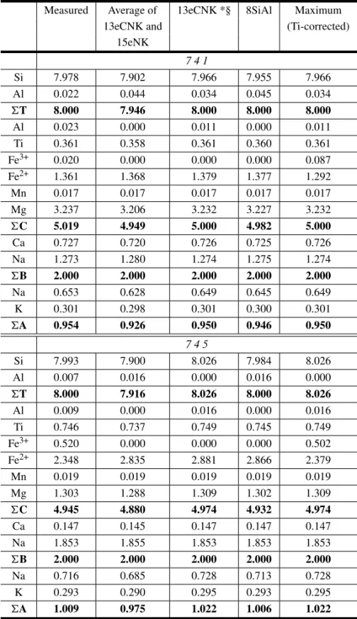
The same four analyses presented by Haw-thorne et al. (1998) were recalculated using the av-erage between 15eNK and 13eCNK, 13eCNK and 8SiAl methods. The results, as well as the measured values, are summarized in Table II.
The comparison reveals that the cation dis-tributions resulting from both 13eCNK and 8SiAl methods are good approximations of the measured values, while 15eNK-13eCNK averages are poor ones. These results nicely show that the choice of the recalculation method is not only important for the determination of Fe2+and Fe3+contents, but also
for the appropriate normalization of the other ions (see also Schumacher 1991).
Either 13eCNK or 8SiAl were selected as the maximum estimates by the method of Schumacher (1997), as indicated on Table II. In the case of sample 745, the choice seems inappropriate, but this is a consequence of the relatively high Li content on the analysis, not considered in a first calculation. When Li is considered, the selected method changes to 8SiAl, a much closer match to
the measured values (Table II).
Although the overall cation distributions are calculated correctly, the Fe3+estimates are clearly
underestimated (Table II). This results from the fact that the actual negative charges sum to more than 46, as considered in the computations.
A correction based on the results of Hawthorne et al. (1998) was devised. The actual number of negative charges is 46 + 2 * (Ti – 0.13); hence, the number of equivalent O is half of this value. Fe3+may then be more adequately estimated using
the equation of Droop (1987). A modification of the method of Schumacher (1997) is also possible. There is no essential alteration in the calculation process, except that, when selecting the minimum and maximum estimates, it is necessary to compare the estimated Fe3+ values instead of the correction
factors, since the Fe3+estimates are no longer a
func-tion of the correcfunc-tion factors alone.
The corrected values for the data of Hawthorne et al. (1998) are depicted on Table II. While one of the values is a good approximation (sample 745), the other (sample 741) is overestimated. It should be noted however, that the Fe3+contents of this latter
sample is rather low, what leads to larger errors. Ti-corrected results are also shown on Table II, as computed for the selected complete analytical data of the preceding section. It is clearly seen that the corrected results, at least in general, are not better than the uncorrected ones. Specifically in the case of the calcic amphiboles, the corrections worsened the correlation.
Naturally, it is yet to be proven whether the correlation between Ti4+ and O2– deducted for the
Coyote Peak amphiboles (Hawthorne et al. 1998) is of general applicability. Consequently, this correc-tion should be used with caucorrec-tion, only when there is additional, independent evidence of the presence of oxy-amphibole components. In these cases, it is suggested that factor (i) (10SFe3) of the method of Schumacher (1997) be calculated with a maximum of 0.13 Ti cpfu.
TABLE II
Comparison of cationic distributions calculated (basis of 24 [O, OH, F, Cl]) from selected complete analysis of Hawthorne et al. (1998) and those obtained after calculation of Fe3+by selected stoichiometry-based methods
(basis of 23 O).
Measured Average of 13eCNK *§ 8SiAl Maximum
13eCNK and (Ti-corrected)
15eNK
7 4 1
Si 7.978 7.902 7.966 7.955 7.966
Al 0.022 0.044 0.034 0.045 0.034
T 8.000 7.946 8.000 8.000 8.000
Al 0.023 0.000 0.011 0.000 0.011
Ti 0.361 0.358 0.361 0.360 0.361
Fe3+ 0.020 0.000 0.000 0.000 0.087
Fe2+ 1.361 1.368 1.379 1.377 1.292
Mn 0.017 0.017 0.017 0.017 0.017
Mg 3.237 3.206 3.232 3.227 3.232
C 5.019 4.949 5.000 4.982 5.000
Ca 0.727 0.720 0.726 0.725 0.726
Na 1.273 1.280 1.274 1.275 1.274
B 2.000 2.000 2.000 2.000 2.000
Na 0.653 0.628 0.649 0.645 0.649
K 0.301 0.298 0.301 0.300 0.301
A 0.954 0.926 0.950 0.946 0.950
7 4 5
Si 7.993 7.900 8.026 7.984 8.026
Al 0.007 0.016 0.000 0.016 0.000
T 8.000 7.916 8.026 8.000 8.026
Al 0.009 0.000 0.016 0.000 0.016
Ti 0.746 0.737 0.749 0.745 0.749
Fe3+ 0.520 0.000 0.000 0.000 0.502
Fe2+ 2.348 2.835 2.881 2.866 2.379
Mn 0.019 0.019 0.019 0.019 0.019
Mg 1.303 1.288 1.309 1.302 1.309
C 4.945 4.880 4.974 4.932 4.974
Ca 0.147 0.145 0.147 0.147 0.147
Na 1.853 1.855 1.853 1.853 1.853
B 2.000 2.000 2.000 2.000 2.000
Na 0.716 0.685 0.728 0.713 0.728
K 0.293 0.290 0.295 0.293 0.295
TABLE II (continuation)
Measured Average of 13eCNK *§ 8SiAl Maximum
13eCNK and (Ti-corrected)
15eNK
7 4 9
Si 7.905 7.814 7.907 7.934 7.934
Al 0.066 0.065 0.066 0.066 0.066
T 7.971 7.879 7.972 8.000 8.000
Al 0.000 0.000 0.000 0.000 0.000
Ti 0.438 0.433 0.438 0.439 0.439
Fe3+ 0.000 0.000 0.000 0.000 0.000
Fe2+ 1.557 1.539 1.557 1.563 1.563
Mn 0.032 0.032 0.032 0.032 0.032
Mg 3.000 2.965 3.000 3.011 3.011
C 5.027 4.969 5.028 5.045 5.045
Ca 0.854 0.845 0.855 0.857 0.857
Na 1.146 1.155 1.145 1.143 1.143
B 2.000 2.000 2.000 2.000 2.000
Na 0.659 0.628 0.660 0.669 0.669
K 0.277 0.274 0.277 0.278 0.278
A 0.936 0.902 0.936 0.947 0.947
7 5 0
Si 7.947 7.785 7.942 7.959 7.959
Al 0.041 0.040 0.041 0.041 0.041
T 7.988 7.825 7.982 8.000 8.000
Al 0.000 0.000 0.000 0.000 0.000
Ti 0.643 0.630 0.643 0.644 0.644
Fe3+ 0.000 0.000 0.000 0.000 –0.000
Fe2+ 2.144 2.101 2.143 2.148 2.148
Mn 0.042 0.041 0.042 0.042 0.042
Mg 2.191 2.147 2.190 2.194 2.194
C 5.020 4.919 5.018 5.029 5.029
Ca 0.767 0.751 0.766 0.768 0.768
Na 1.233 1.249 1.234 1.232 1.232
B 2.000 2.000 2.000 2.000 2.000
Na 0.664 0.610 0.662 0.668 0.668
K 0.288 0.282 0.287 0.288 0.288
A 0.952 0.891 0.950 0.956 0.956
significant, especially for igneous amphiboles. If this substitution is important, the preceding analy-sis suggests that Fe3+ will be underestimated, but
the overall cation distributions can be well approxi-mated by proper choice of calculation procedure.
CATION DISTRIBUTIONS AND IMPLICATIONS FOR THE IMA CLASSIFICATION
It has been conclusively demonstrated (Schumacher 1991) that cation distributions including Fe3+ and Fe2+estimates result in much better approximations to the expected values than the uncorrected results. The resulting partitioning of elements occurring in more than one site (e.g. Al in T and C sites), on the other hand, is very sensitive to the calculation procedure.
These two findings are nicely demonstrated by the results on Table II. For example, total Al con-tents in sample 741 are well predicted by all models. Nevertheless, none of them leads to good approxi-mations of the measuredIVAl-VIAl partitioning. The same is true for partial sums (e.g. C- and A-sum; Table II).
It should be noted that the parameters used in the IMA classification (Leake et al. 1997) are either the contents of an element present in more than one site, or partial sums:IVAl, Na
B, [Na+K]A,VIAl/Fe3+
ratio. In this sense, the classification is strongly model-dependent (see also Schumacher 1997), and it follows that a range of names is possible for any given analysis. Evidently, this difficulty will persist until a method that allows the determination of Fe3+
at the micrometer scale and can be used routinely is available.
CONCLUSIONS
Although several authors have strongly criticized the estimation of Fe3+and Fe2+through
stoichiomet-ric calculations (e.g. Hawthorne 1983, Czamanske and Dillet 1988), these kinds of calculation are not only desirable, but also necessary, considering the existing volume of available microprobe amphibole analyses and the general employment of the EPMA as the standard microanalytical tool.
It has been shown here that the quality of the results is strongly dependent on the choice of the crystallochemical criterion, and this choice depends primarily on the amphibole group of interest. This is in accordance with the conclusions of previous workers (Robinson et al. 1982, Schumacher 1997). For calcic, sodic-calcic, and sodic amphiboles, 13eCNK estimates are, in general, satisfactorily precise and accurate. In some instances, however, other crystallochemical criteria, namely 8SiAl and 15eK, lead to more appropriate results. In these cases, the method of Schumacher (1997) correctly identifies the best minimum and maximum es-timates. Yet, as the actual values are much closer to the maximum estimates than to the minimum ones, the use of the average between them is not adequate. It is recommended, thus, that for calcic, sodic-calcic, and sodic amphiboles, the maximum estimates of the method of Schumacher (1997) be used instead of the average ones.
Fe3+ is underestimated when the
oxy-amphi-bole component is present, even though the overall cationic distribution is correctly calculated. A cor-rection procedure is proposed here, but it should be applied with caution, since it is based on data on a single suite of rocks of very particular origin (Cza-manske and Atkin 1985, Hawthorne et al. 1998).
The program MINCAL may be obtained from the authors.
ACKNOWLEDGMENTS
We are indebted to V. Janasi, L. Martins and M. Ulbrich for their comments and suggestions. Com-ments by J. Schumacher and R. Dymek helped im-prove the manuscript. G. Gualda benefited from a M.Sc. scholarship from the Fundação de Ampa-ro à Pesquisa do Estado de São Paulo (FAPESP-98/15656-7).
RESUMO
calcu-ladas, não existe critério único que possa ser usado para anfibólios.
Um grande número de análises de anfibólios cálcicos, sódico-cálcicos e sódicos de granitos e sienitos Tipo-A aflorantes no Sul do Brasil foi utilizado para avaliar as escolhas feitas pelo método de Schumacher (1997, Cana-dian Mineralogist, 35: 238-246), que utiliza a média entre estimativas máximas e mínimas selecionadas. As estima-tivas selecionadas com maior freqüência são: 13 cátions excluindo Ca, Na e K (13eCNK – 66%); soma de Si e Al igual a 8 (8SiAl – 17%); 15 cátions excluindo K (15eK – 8%). Estas estimativas são apropriadas tomando por base critérios cristaloquímicos. Estimativas mínimas são principalmente todo ferro como Fe2+(allFe2 – 71%) e se mostram claramente inadequadas. Portanto, estimativas máximas devem aproximar melhor os valores verdadeiros.
Como teste, análises completas foram selecionadas da literatura, e valores calculados e medidos foram com-parados. Estimativas 13eCNK e máximas são precisas e exatas (coeficiente de concordância – rc≈ 0.85). As médias, em contrapartida, aproximam mal os valores me-didos (rc= 0.56).
Recomenda-se, portanto, que as estimativas máximas do método de Schumacher sejam utilizadas para anfibólios cálcicos, sódico-cálcicos e sódicos.
Palavras-chave:anfibólios, estequiometria, ferro férrico, EPMA.
REFERENCES
Bastin GV, van Loo FJJ and Heijligers HJM.1984.
Evaluation and use of Gaussianφ (ρz)curves in quan-titative electron probe microanalysis: a new opti-mization. X-ray Spectr 13: 91–97.
Cosca MA, Essene EI and Bowman JR.1991.
Com-plete chemical-analyses of metamorphic hornblendes – implications for normalizations, calculated H2O activities, and thermobarometry. Contrib Mineral Petrol 108: 472–484.
Czamanske GK and Atkin SA. 1985.
Metasoma-tism, titanian acmite, and alkali amphiboles in lithic-wacke inclusions within the Coyote Peak diatreme, Humboldt-county, California. Amer Mineral 70: 499–516.
Czamanske GK and Dillet B.1988. Alkali amphibole,
tetrasilicic mica, and sodic pyroxene in peralkaline siliceous rocks, Questa Caldera, New Mexico. Amer J Sci 288A: 358–392.
Deer WA, Howie RA and Zussman MA.1992. An
introduction to the rock-forming minerals, 2nd ed., London: Longman, 696 p.
Deer WA, Howie RA and Zussman MA.1997.
Rock-forming minerals: Double-Chain Silicates, 2nded., London: Logman, v. 2B, 668 p.
Delaney JS, Bajt S, Sutton SR and Dyar MD.1996.
In situmicroanalysis of Fe3+/σFe in amphibole by
x-ray near edge structure (XANES) spectroscopy. In: Dyar MD, McCammon C and Shaeffer MW
(Eds), Mineral spectroscopy: A tribute to Roger E. Burns. Geochem Soc Spec Public 5: 165–171.
Droop GTR.1987. A general equation for
estimat-ing Fe3+in ferromagnesian silicates and oxides from microprobe analysis, using stoichiometric criteria. Mineral Mag 51: 431–437.
Dyar MD, Mackwell SJ, Mcguire AV, Cross LR and
Robertson JD.1993. Crystal-chemistry of Fe3+and H+ in mantle kaersutite – implications for mantle metasomatism. Amer Mineral 78: 968–979.
Enders M, Speer D, Maresch WV and McCammon
CA. 2000. Ferric/ferrous iron ratios in sodic
am-phiboles: Mössbauer analysis, stoichiometry-based calculations and the high-resolution microanalytical flank method. Contrib Mineral Petrol 140: 135–147.
Gualda GAR.2001. Evolução petrográfica e
mineraló-gica das associações alcalina e aluminosa dos Grani-tos Tipo-A da Graciosa, PR. MSc dissertation, Insti-tuto de Geociências, Universidade de São Paulo, SP, Brasil, 271 p.
Hawthorne FC. 1983. The crystal-chemistry of the
amphiboles. Can Mineral 21: 173–480.
Hawthorne FC, Oberti R, Zanetti A and
Cza-manske GK. 1998. The role of Ti in
hydrogen-deficient amphiboles: Sodic-calcic and sodic amphi-boles from Coyote Peak, California. Can Mineral 36: 1253–1265.
Holland Y and Blundy J. 1994. Non-ideal
inter-actions in calcic amphiboles and their bearing on amphibole-plagioclase thermometry. Contrib Min-eral Petrol 116: 433–447.
King PL, White AJR, Chappel BW and Allen CM.
Lameyre J and Bowden P.1982. Plutonic rock type
series: discrimination of various granitoid series and related rocks. J Volcan Geoth Res 14: 169–189.
Leake BE, Wooley AR, Arps CES, Birch WD,
Gil-bert MC, Grice JD, Hawthorne FC, Kato A,
Kisch HJ, Krivovichev VG et al. 1997.
Nomen-clature of amphiboles: report of the Subcommittee on Amphiboles of the International Mineralogical Asso-ciation Commission on New Minerals and Mineral Names. Can Mineral 35: 219–237.
Lin LI.1989. A concordance correlation-coefficient to
evaluate reproducibility. Biometrics 45: 255–268.
Martins L.2001. Condições de cristalização de granitos
sin- e tardi-orogênicos da porção central do Batóli-to Agudos Grandes, SP, com base em geoquímica de minerais e rochas. MSc dissertation, Instituto de Geociências, Universidade de São Paulo, SP, Brasil, 132 p.
Papike JJ, Cameron KL and Baldwin K.1974.
Amphi-boles and pyroxenes; characterization of other than quadrilateral components and estimates of ferric iron from microprobe data. Geol Soc Amer Abs Prog 6: 1053–1054.
Robinson P, Spear F, Schumacher JC, Laird J, Klein
C, Evans BW and Dooland BL.1982. Phase
re-lations of metamorphic amphiboles: natural occur-rences and theory. Rev Mineral 9B: 69–76.
Schumacher JC.1991. Empirical ferric iron
correc-tions: necessity, assumptions and effects on selected geothermobarometers. Mineral Mag 55: 3–18.
Schumacher JC.1997. Appendix 2: the estimate of
ferric iron in electron microprobe analysis of amphi-boles. Can Mineral 35: 238–246.
Stout JH.1972. Phase petrology and mineral chemistry
of coexisting amphiboles from Telemark, Norway. J Petrol 13: 99–146.
Sutton SR, Delaney JS, Bajt S, Rivers ML and
Smith JV. 1993. Microanalysis of iron oxidation
state in iron oxides using X-ray absorption near edge structure (XANES). In: Lunar and Planetary Science, Lunar and Planetary Institute 24: 1385–1386.
Vlach SRF, Janasi VA and Vasconcellos ACBC.
1990. The Itu Belt: associated calc-alkaline and alu-minous A-type late Brasiliano granitoids in the States of São Paulo and Paraná, southern Brazil. In: Con-gresso Brasileiro de Geologia, 36, Natal, RN,
![Fig. 1 – Na B versus [Ca+Na] B classification plot (after Leake et al. 1997) showing the array variation from calcic to sodic-calcic, and sodic among the amphiboles of the Graciosa A-type Granites, southern Brazil](https://thumb-eu.123doks.com/thumbv2/123dok_br/15968687.686852/4.918.476.831.376.614/classification-showing-variation-amphiboles-graciosa-granites-southern-brazil.webp)