Close range ship noise cross correlations with a vector sensor in view of geoacoustic inversion

Close range ship noise cross correlations with a

vector sensor in view of geoacoustic inversion

Yanqun Wu

1,2

1 _{Laboratory of Robotics and Systems in Engineering and} Science (LARSyS), University of Algarve, Campus de Gambelas, 8005-139 Faro, Portugal

2 _{Academy of Ocean Science and Engineering, National} University of Defense Technology, Changsha 410073, P.R. China

Ana Bela Santos, Paulo Felisberto, Sergio M. Jesus

Laboratory of Robotics and Systems in Engineering and Science (LARSyS), University of Algarve, Campus de

Gambelas, 8005-139 Faro, Portugal

Abstract—Distant ship noise has been utilized for geoacoustic

inversion and ocean monitoring for many years. In a shallow water experiment, Makai 2005, a 4-element acoustic vector sensor array was deployed at the stern of the research vessel R/V Kilo Moana. The recorded engine noise of R/V Kilo Moana during its dynamical positioning was analyzed by the DEMON (Detection of Envelope Modulation on Noise) method. The strongest modulation frequency band of the ship noise was found by a group of band-pass filters for further data processing. Multipath arrivals in the vertical particle velocity have higher signal-to-noise ratios than those in the horizontal particle velocities because of steep arrival directions. By exploiting this advantage, the cross correlation of the broadband ship noise between the pressure and the vertical particle velocity can be used for multipath information exploration. Since the ship noise is often characterized as continuous broadband noise plus strong tonal noise, the cross correlation of the tonal noise would dominate that of the broadband noise, and consequently cover the multipath arrival pattern. Therefore, the spectral weighting functions are applied to reduce the noise contamination and ensure sharp multipath peaks in the cross correlation. For the engine noise emitted by the dynamically positioned ship, a short correlation time of 0.4s was used in order to keep the time delay fluctuation details of multipath arrivals. Clear multiple arrivals are seen in the cross correlation of different arrivals, and verified by the ray tracing program TRACEO. The results demonstrate the potentials of only one acoustic vector sensor in applications of source localization and geoacoustic inversion.

Keywords—vector sensor, cross correlation, geoacoustic inversion, ship noise

I. INTRODUCTION

Geoacoustic inversion of the ocean bottom is of great interest nowadays due to its economy and low consumption in time. An acoustic vector sensor (AVS), manifesting itself great potential for underwater measurements, is a combined sensor with one pressure sensor and one two or three dimensional particle velocity or accelerometer. It has been demonstrated the great potential of AVSs in underwater acoustic measurements because of its inherent directivity to resolve directional ambiguity and increased gain against isotropic and directional noise over the pressure sensor [1],[2],[3], etc. Furthermore, source localization and geoacoustic inversion can be realized

by a single AVS or an AVS array, which is a great benefit for space limited vehicles, and the results were also improved compared to the pressure only array by utilizing the vertical particle velocity [2],[4]~[8].

Recent trends of utilizing passive acoustic sources, such as ambient noise and ships of opportunity noise, to infer seabed layering and seabed geoacoustic properties are increasing. Cross correlating ambient noise by separated hydrophones can extract the impulse response or Green's function from one hydrophone to the other [9],[10]. Furthermore, cross correlation of surface ship noises can also be used for the multipath time delay estimation and the ship localization by spatially spaced hydrophones [12]. An AVS samples the pressure and the three-dimensional particle velocity at one point, and thus gives four auto- correlations and twelve cross correlations which provide more information for source localization and geoacoustic inversion. As a matter of fact, the peaks of the cross correlation between the particle velocity and the pressure components includes the multipath time delays for the source positions and magnitudes for the bottom reflection coefficients.

The paper investigates the cross correlations of close range ship noise between the pressure and the particle velocity components for multipath information exploration. Ship noise was identified first by the DEMON (Detection of Envelope Modulation on Noise) spectrum, and then the weighting functions in the family of the generalized cross-correlation (GCC) are applied to emphasis the low SNR ship noise and sharp the multipath peaks in the cross correlation. Simulations are conducted to analyze the multipath arrivals and validate the benefit of the vertical particle velocity in the near field.

II. SHIP NIOSE IDENTIFICATION IN MAKAI 2005

A. Makai 2005

The Makai experiment took place from 15 Sep to 2 Oct 2005, near the coast of Kauai, Hawaii. Makai 2005 was the third experiment for high frequency ocean acoustic research, which involves high-resolution tomography, high frequency propagation modeling and acoustic communications. It was organized by HLS and sponsored by ONR, involved a large number of international teams both from government and

international labs, universities and private companies, such as HLS, UALg, UDEL, SPAWAR, NRL, NURC, etc[13]. During the Makai experiment, a four-element AVS array was vertically suspended close to the stern of the research vessel R/V Kilo Moana to collect data from towed and fixed acoustic sources. The AVS array of 10cm spacing consisted of TV-001 type sensors from the Wilcoxon company, which is a combined sensor with one omni-directional hydrophone and three uniaxial accelerometers arranged in a tri-axial configuration[8]. The length of the AVS array was 0.3m and it was deployed with the deepest sensor of depth 79.9m, as shown in Fig. 1. This selected environment has a deep mixed layer and negative sound speed profile, and the bathymetry at the site is range independent with a water depth of around 104 m.

Fig. 1. The AVS array configuration in Makai 2005

B. Ship noise identification by DEMON Spectrum

The vessel R/V Kilo Moana has an overall length of 57m and beam length of 27m, and full-load draft of 7.5m. She incorporates a sophisticated dynamic positioning system (DPS) which accepts data input from position and environmental sensors and automatically controls propulsion and steering to perform precise maneuvers. On the first day of the trial for the AVS array, that is Julian day 264, R/V Kilo Moana used the DPS to keep itself at the same location and thus its motor engine ran for a few seconds every few minutes, whose noise was heard in the recorded AVS array data.

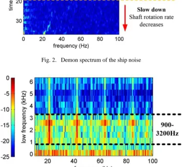
From the spectrogram of these data, there were a lot of tones below 1kHz and weak noise above 3.5kHz, which is not good for the cross correlation. Its DEMON (Detection of Envelope Modulation on Noise) spectrum is shown in fig. 2 that the modulation frequency increased when the engine speeded up, and decreased when the engine slowed down. At 7.8sec, the fundamental frequency is around 21.24Hz. In the specification sheet of R/V Kilo Moana, it is reported its bow thruster motor is rated 1150 HP, 1200 RPM, i.e. 20Hz [14]. This information verifies the demodulation result.

Since the propeller noise was modulated on the broadband ship noise, the frequency band of ship noise that is most strongly modulated can be estimated. The purpose here is to find the desired ship noise frequency band for the following analysis. In order to do that, the signal at 7.8sec is selected, and filtered by several band pass filters with the frequency band of 500Hz, that is frequency band from 100Hz to 600Hz, 600Hz to 1100Hz, etc. The DEMON spectrums were stacked along the

center frequencies of different filters as shown in fig. 3. It is seen that the demodulated signal in frequency band 900-3200Hz has the strongest amplitudes. Therefore, this frequency band is chosen as the desired ship noise band in the following sections.

Fig. 2. Demon spectrum of the ship noise

Fig. 3. DEMON spectrums stacked by the different bandpass filters with the bandwith of 500Hz and the vertical axis denotes the lower frequencies of the bandpass filters.

III. MULTIPATH CROSS CORRELATION WITH A VECTOR SENSOR FOR GEOACOUSTIC INVERSION

A. Multipath cross correlation with a vector sensor

Since the pressure and the particle velocity components of an AVS are co-located, each eigenray arrives at four components of the AVS at the same time. For a vertical AVS array without tilting or any movement, a point source can be viewed in the xoz or yoz plane of the AVS array, which means all eigenrays have the same azimuth angle



_s of the desired source but different elevation angles of rays from different launching angles.

Harmonic tones are always considered as a nuisance that destroy the broadband peaks in the cross correlation. At the same time, the high background colored noise makes the SNR of the received channels rather low and then the multipath peaks in the cross correlation are smeared. Therefore, before cross correlation, time and frequency normalization methods are utilized before the cross correlation as shown in fig.4 to reduce these harmonic noises and emphasize desired signals

Fig. 4. Flowchart of the whitened cross correlation

The absolute whitening (AW) or the spectral whitening (SW) method in the frequency domain is widely applied and demonstrated effective in seismology interferometry. It replaces the cross spectrum with a unit amplitude spectrum, that is [10]

 

 

 

n n n

Y



X



X



(1) where X_n

 



is the spectrum of the n nth( 1, 2,3, 4)

component in the AVS.

Let the q_th component of one AVS be the reference channel, the cross spectrum between the n_th and the q_th components is given by

 

   

*

nq n q

C



Y



Y



(2) Where  is the conjugation operator. After inverse Fourier transformation (IFT) of C_nq

 



, the new cross correlation

 

nq

c



can be obtained.

The generalized cross-correlation (GCC) method for time delay estimation (TDE) is a popular technique which reshapes the cross spectrum by frequency weighting functions [15]. The most well-known weighting functions in the GCC family are the Phase Transform (PHAT), the Smoothed Coherence Transform (SCOT), and the ROTH, etc. The purpose of these weighting functions is to reduce the noise contamination and ensure a large sharp peak in the cross correlation It is shown that GCC is quite successful in extracting time delays between different sensors in an open-field environment where no multipath or reverberation effect is present. In the multipath environment, we may apply these frequency weighting functions to emphasize the low SNR ship noise.

Let W

 



be the weighting function, the GCC is given by

[15]

 

   

nq nq

G



C



W



(3) Where W

 



1 Cnq

 



is for the PHAT method;

 

1 qq

 

W



 C



for the ROTH method;

 

1 nn

   

qq

W



 C



C



for the SCOT method.

The PHAT is free from the source signal and depends only on the channel responses, which is similar to the AW processor. The numerical differences between the AW of the time-series prior can be neglected [11]. The ROTH has a desirable effect of suppressing those frequency regions where the noise is large. The SCOT assigns weight according to signal and noise

characteristic, and is a compromise between the PHAT and ROTH preprocessors.

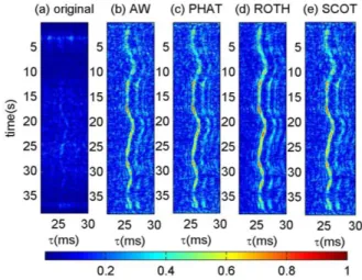
Fig. 5. Comparison of cross correlations between p and vz of the first AVS with different data preprocessing techniques: (a) orginal; (b)AW; (c)PHAT;

(d)ROTH; (e)SCOT.

(a) Normalized cross correlations between the pressure and the other components of the first AVS

(b) Normalized cross correlations between the pressure component of the first AVS and all the components of the second AVS

Fig. 6. Comparison of cross correlations between different components of one AVS and different AVSs using the ROTH method

In the data processing, the pressure component of the first AVS can be selected without loss of generality. As shown in fig. 5, all these whitening techniques are effective in improving the multipath peaks compared with the original cross correlation in

fig. 5(a). The ROTH has the lowest sidelobes among all the preprocessors since there is very strong harmonic ship noise in our data.

In the near field, the vertical particle velocity component of an AVS has higher signal-to-noise ratios than its horizontal components for multiple reflected arrivals because of steep elevation angles. Then the cross correlations between the pressure (p(1)) and the horizontal particle velocities vx (vx (1))

and vy (vy(1)) of the first AVS have smaller multipath peaks and

higher sidelobes than that between the pressure and vz (vz(1))

after the ROTH normalization, which is shown in fig. 6(a). The peak of the auto-correlation, that is p(1)-p(1) in fig. 6(a), is rather ambiguous due to the fact that the normalization process will destroy the multipath information in the auto-correlation. According to [4], the cross correlation peak will shift and its sign will change as well under the low SNR, and that is why the positions of peaks of the cross correlations between different components in fig. 6(a) are slightly different. Nevertheless, fig. 6(b) shows the normalized cross correlation between p(1) and the second vertical particle velocity (vz(2)) is

in phase with that between p(1) and the second pressure (p(2)), while the cross correlation between p(1) and vx(2) is in phase

with that between p(1) and vy (2).

B. Multipath time delay identification in Makai 2005

Since the relative positions of the ship to the AVS array is roughly known, an attempt is made to understand where the cross correlation peaks come from. Simulations using Makai setup are performed by the ray model Traceo[15] in the following. It is reasonable to assume that all possible ship positions are in the region of the depth and range of [0,15] m×[1,120]m. Cross correlations in this region are three dimensional, and slices of the cross correlations between the 1st and 2nd pressure sensors at a fixed source range of 50m and a fixed source depth of 7m are taken as examples and shown in figs. 7 and 8.

Fig. 7. Cross correlation at source range 50m and different source depths, where D,S,B denote the direct, the surface reflected and the bottom reflected

paths; and the prime denotes the second receiver.

As shown in figs. 7 and 8, there should be strong peaks related to surface reflected paths. However, fig.5 shows no surface reflected paths in the Makai results. The possible reason is the ship is too close to the AVS array that the first few surface reflected paths happen inside the ship, which may attenuate energies of eigenrays related to the surface reflected

paths. Then after removing the surface reflected paths in figs. 7 and 8, we can find that it is impossible to satisfy both time delays around 26ms and 27ms for all possible source positions unless the source is very deep or very far from the AVS array. Therefore, the possible conclusion for these two arrivals is they come from the bottom and sub-bottom reflected paths, from where the first bottom layer depth can be inferred.

To validate the application of the vertical particle velocity vz in the near field, the cross correlations between the pressure and the horizontal particle velocity vr and the pressure and vz are shown in fig. 9. It can be seen that the cross correlation between p and vz is stronger and has better SNR than that between p and vr, which verifies the Makai results.

Fig. 8. Cross correlations at different source ranges and source depth 7m.

Fig. 9. Cross correlations between p and vr and p and vz with both normlized by the maximum value of the cross correlation between p and vz at source

range 50m and depth 2m.

IV. CONCLUSION

In the paper, the multipath cross correlation between the pressure and the particle velocities for the purpose of the geoacoustic inversion is discussed. The noise of the research vessel R/V Kilo Moana in close range was identified by the DEMON method, which is consistent with its specification. It is found through Makai results and simulations that multipath arrivals in the vertical particle velocity have higher signal-to-noise ratios than those in the horizontal particle velocities because of steep arrival directions. Further analyses infer that there are possible multiple layers by the cross correlation of the broadband ship noise between the pressure and the vertical particle velocity. The results demonstrate the potentials of only one AVS for the bottom layer depth estimation.

ACKNOWLEDGMENTS

The authors would like to thank Michael Porter, chief scientist for the Makai Experiment, Jerry Tarasek for the loan of the vector sensor array used in the experiment and Paul Hursky, Martin Siderius and Bruce Abraham for providing assistance with the data acquisition. The Makai Experiment was supported by the US Office of Naval Research.

REFERENCES

[1] J. C. Shipps and B. M. Abraham, “Safe waters make sense,” Sensors Defend The Plant, pp.39-40, December 2004.

[2] L. Gerald, J.C. Luby, G.R. Wilson, and R.A. Gramann, “Vector sensors and vector sensor line arrays: Comments on optimal array gain and detection,” J. Acoust. Soc. Am., 2006, vol.120, no.1, pp.171-185. [3] Yanqun Wu, Zhengliang Hu, Hong Luo, and Yongming Hu, “Source

number detectability by an acoustic vector sensor linear array and performance analysis,” IEEE J. Oceanic Eng., vol.39, no.4, pp. 769-778, 2014.

[4] P. Felisberto, O. Rodriguez, P. Santos, E. Ey, and S.M. Jesus, “Experimental results of underwater cooperative source localization using a single acoustic vector sensor,” Sensors, vol. 13, no. 7, pp.8856-8878, 2013.

[5] P. Santos, O. Rodriguez, P. Felisberto, and S.M. Jesus, “Seabed geoacoustic characterization with a vector sensor array,” J. Acoust. Soc. Am., vol.128, no.5, pp. 2652-2663,2010.

[6] J.P. Hermand, M. Berrada, and M. Asch, “Particle velocity in geoacoustics: A performance study based on ensemble adjoint inversion,” 2010.

[7] A.K. Robert, “Proof of principle for inversion of vector sensor array data,” J. Acoust. Soc. Am., vol.128, no.2, pp.590-599, 2010.

[8] P. Santos, “Ocean parameter estimation with high-frequency signals using a vector sensor array,” Ph. Disertation, Universidade do Algarve,2012.

[9] P. Roux, W. A. Kuperman, and the NPAL Group, “Extracting coherent wave fronts from acoustic ambient noise in the ocean,” J. Acoust. Soc. Am., vol.116, no.4, pp. 1995-2003, 2004.

[10] L.A. Brooks, and P. Gerstoft, “Green's function approximation from cross-correlations of 20-100 Hz noise during a tropical storm,” J. Acoust. Soc. Am., vol. 125, no. 2, pp.723-734, 2009.

[11] J.C. Groos, S. Bussat and J.R.R. Ritter, “Performance of different processing schemes in seismic noise cross-correlations,’’ Geophysical Journal International, vol. 188, pp. 498-512, 2012.

[12] J. Gebbie, M. Siderius, R. McCargar, J.S. Allen III, and G. Pusey, “Localization of a noisy broadband surface target using time differences of multipath arrivals,” J. Acoust. Soc. Am., vol.134, no.1, EL77-EL83, 2013.

[13] M. Porter, B. Abraham, M. Badiey, M. Buckingham, T. Folegot, P. Hursky, S. Jesus, et al. The Makai experiment: High frequency acoustics. Proceedings of the 8th ECUA European Conferece on Underwater Acoustic, Carvoeiro, Portugal, 12–15 June 2006; Volume 1, pp. 9-18.. [14] ftp://soest.hawaii.edu/pibhmc/outgoing/SOW%20Rev%205/Appendix%

20C%20-20Bow%20Thruster%20Drive%20System,%20Rev%201%20-%2008-08-14.doc

[15] G.C. Carter, “Coherence and time delay estimation,” Proceedings of the IEEE, vol.75, no.2, pp.236-255,1987.

[16] O. Rodriguez, “The TRACE and TRACEO ray tracing programs,” http://www.siplab.fct.ualg.pt/models.shtml.