UNIVERSIDADE DO ALGARVE
FACULDADE DE CIÊNCIAS E TECNOLOGIA
Localização de Soluções para
Equações de Navier-Stokes Planares
Hermenegildo Augusto Vieira Borges de Oliveira (Mestre)
Dissertação para a obtenção do Grau de Doutor em Matemática, Especialidade de Análise Matemática
u
Faro, Janeiro de 2004 TESES
i híímíji
UNIVERSIDADE DO ALGARVE
FACULDADE DE CIÊNCIAS E TECNOLOGIA
u
/ Xx t* t
n/
VW x/
Localização de Soluções para
Equações de Navier-Stokes Planares
Hermenegildo Augusto Vieira Borges de Oliveira (Mestre)
Dissertação para a obtenção do Grau de Doutor era Matemática, Especialidade de Análise Matemática
OU + ioC d '
UNIVERSITY OF ALGARVE
FACULTY OF SCIENCES AND TECHNOLOGY
Localization of Solutions for Planar Navier-Stokes Equations
Hermenegildo Augusto Vieira Borges de Oliveira (Master)
Dissertation to obtain the degree of Ph.D. in Mathematics, Speciality of Mathematical Analysis
u
t*
ERRATA
"Localization of solutions for planar Navier-Stokes equations" Hermenegildo Borges de Oliveira
July 13, 2004
p. 4 To replace in equation (1.1.6) "... for any g > 0 ..." by "... for any g > 1 ...".
p. 6 To replace in Theorem (Lebesgue) "... limn_00 fí2 fn{x) dx = fQ f{x) dx." by "... |/n —/li^n)
converges to zero.", and to add the the following result
Corollary Let /„ be a monotone increasing sequence of non-negative real measurable, but not necessarily integrable, functions converging almost everywhere to a function f. Then
Um / fn{x)dx= / f{x)dx.
"-+00 Jçi Jçi
p. 26 In Theorem 2.4.1 to replace "... s G [1,2) ..." by "... s G (0,1) ...".
p. 27 The reasoning at the end of the page must be corrected as follows: a) four Unes above "... Ag(x, vN) ..." is replaced by "... Ag(x, wN) ..."; b) one Une above, "... we obtain the estimate
..." is replaced by "... we obtain the a priori estimate ..."; c) equation (2.4.40) is corrected to "... [[w^Hni^N) < C, where C = C {L,p,s,u,R) ..."; d) continuing on p. 28, in the first Une, "... maps L2(í2Ar) x [0,1] ..." is replaced by "... maps a bali in L2(í2Af) x [0,1] ...".
p. 29 To replace, at the end of the fifth Une, counting from the bottom, "... with Ag(x, v^) ..." by "... with Ag(x, w^) in the third, from the bottom, "... the estimate (2.4.40) ..." by "... the a priori estimate (2.4.40) ...", and, in the last Une, "... C = C ^L, u,R, ||a||LTa_ , ||ft||L2(njv), ||vw
..." by "... C = C i/,i?, ..."- Continuing on p. 30, in the third Une, to replace "... maps L2(í)iV) x [0,1] ..." by "... maps a bali in L2(í^)x[0,l] ...".
p. 42 To correct, in the fourth Une, "... C5 < C3C£ ll+C4 < 0." to "... C5 < C3CÇ
C4.".
p. 61 In the first Une above equation (4.3.26), to replace "... s G [1,2) ..." by "... s G (0,1) ...". p. 63 In Theorem 4.3.2 to replace "... for any A < A* and for some smail enough positive constant
A* > 0." by "... for some small enough positive constant A > 0.".
p. 72 In the first Une below equation (5.1.6), we must supplement that sentence with ", if we are considering u = u* on a; = 0,".
Título: Localização de soluções para equações de Navier-Stokes planares. Nome: Hermenegildo Augusto Vieira, Borges de Oliveira.
Doutoramento: Ramo de Matemática, especialidade de Análise Matemática. Orientador: Stanislav Nikolaevich Antontsev. Professor Catedrático.
Resumo
Consideramos escoamentos de fluidos viscosos incompressíveis, em faixas semi-infinitas horizontais, governados pelos sistemas estacionários de Stokes, Naviei-St,okes e Boussi- nesq. Nos problemas de Stokes |6, 7, 8] e Navier-Stokes |9, 14), consideramos condições de fronteira nulas nas paredes horizontais, velocidades possivelmente não nulas nas entradas das faixas e consideramos velocidades nulas no infinito. Para o problema de Boussinesq |I0|. consideramos o sistema formado pelas equações de Navier-Stokes, com as condições de fronteira anteriormente mencionadas, e pela equação estacionária para a temperatura, com temperatura possivelmente não nula na. fronteira compacta e temperatura nula no infinito. Mostramos como estes fluidos podem ser parados a uma distância finita das entradas das faixas por meio de um campo de forças dissipa- tivo com memória dependendo de um modo sublinear da velocidade. ( onsideramos também um escoamento planar de um fluido viscoso incompressível, num domínio re- sultante do produto de uma faixa, semi-infinita horizontal com o intervalo de tempo (O.oo), governado pelo sistema, de Navier-Stokes evolutivo |11, 13]. Neste caso. consi- deramos condições de fronteira nulas na fronteira, compacta, velocidade nula no infinito e uma. velocidade inicial possivelmente não nula. Para este caso, mostramos como este fluido pode ser parado num tempo finito. Todas esta propriedades são denominadas por efeitos de localização e são demonstradas reduzindo os problemas considerados a outros, não lineares do tipo bi-harmónico, para os quais a localização das soluções é obtida por aplicação de um método de energia apropriado. Como a presença dos ter- mos não lineares definidos através dos campos de forças não é habitual em literatura de Mecânica, dos Fluidos, estabelecemos também alguns resultados de existência e uni- cidade de soluções fracas para estes problemas. Finalmente, fazemos uma, incursão da aplicação dos nossos resultados em Elasticidade ( lássica, Hidrodinâmica Magnética e Escoamentos Quase-Geostróficos.
Palavras-chave
Domínios planares, sistema de Stokes estacionário, sistema de Navier-Stokes estacio- nário. sistema de Boussinesq estacionário, sistema de Navier-Stokes evolutivo, campo de forças dissipativo com memória, efeitos de localização, métodos de energia.
Title: Localization of solutions for planar Navier-Stokes equations. Name: Hermenegildo Augusto Vieira Borges de Oliveira.
Ph. D.: Brandi of Mathematics, spedality oí Mathematical Analysis. Supervisor: Stanislav Nikolaevich Antontsev, Full Professor.
Abstract
We consider planar flows of incompressible viscous fluids, in semi-iníinite horizontal strips, governed by the stationary Stokes, Navier-Stokes and Boussinesq systems. In the Stokes [6, 7, 8] and Navier-Stokes |9, 14| problems, we consider zero boundary con- ditions on the lateral walls, possible non-zero velocities at the strip entrances and we prescribe zero velocities at infinity. For the Boussinesq problem [10], we consider the Navier-Stokes equations supplemented with the aforementioned boundary conditions, and we consider the coupled stationary equation for the temperature added with a possible non-zero temperature on the compact boundary and with a prescribed zero temperature at infinity. We show how these fluids can be stopped at a finite distance from the strip entrances by means of feedback dissipative íields depending in a sub- linear way on the velocity field. We consider also a planar how of an incompressible viscous fluid, in a domain resulting from the product of a horizontal semi-infinite strip with the time interval (0,oo), governed by the evolutionary Navier-Stokes |11, 13] sys- tem. In this problem, we consider zero boundary conditions on the compact boundary, zero prescribed velocity at infinity and a, possible non-zero initial velocity. For this case, we show how this fluid can be stopped in a finite time. Ali these properties are denoted as localization effects and are proved reducing the considered problems to non-lmear bi-harmonic types for which the localization of solutions is obtained by means oí the application of a suitable energy method. Since the presence of the non-linear terms deíined through the body forces fields is not standard in the Fluid Mechanics litera- ture, we establish also some results about existence and uniqueness of weak solutions for these problems. Finally, we make an attempt to apply these results in ( lassical Elasticity, Magneto-Hydrodynamics and Quasi-Geostrophic Flows.
Keywords
Planar problems, stationary Stokes system, stationary Navier-Stokes system, stationary Boussinesq system, evolutionary Navier-Stokes system, feedback dissipative forces field. localization effects, energy methods.
"Ainda que eu tenha o dom da profecia e conheça todos os mistérios e toda a ciência, ainda que eu tenha tão grande fé que transporte montanhas, se não tiver amor, nada sou. "
"And though I have the gift of prophecy, and understand ali mysteries and ali knowledge, and though I have ali faith, so that I could remove mountains, but have not love, I am nothing. "
Acknowledgement s
"Muito obrigado! Bojrbiuoe cnacuôo! Muchas gradas! Thank you very much!"
H.B. de Oliveira. I start by thanking those people who are really important to me, ali my fiiends and colleagues, brothers and sisters, brothers and sisters-in-law, ali my nephews and nieces, parents-in-law, my father and mother, my wife and my son. I thank ali of them, not for their direct contribution for this work, but for their understanding of the time that 1 deprive myself of their fantastic company, my friends, for the strength of always believing in me and their interest in my career, my brothers and parents, for loving me, my wife, and just for his existence, my son. The suspensible tear drop that I left here is yours.
Next I want to express my deep gratitude to Professor S.N. Antontsev for had supervising me during this work, and special for has accepted that in the always difficult condition, for both, which was we working in places more than 500 Km apart, me at University of Algarve and him at University of Beira Interior. I thank him for ali the knowledge, skills and train he gave to me, especially in how to understand these phenomena of Fluid Mechanics from the Physics point of view. I thank him also the facilities he proportioned to me at University of Beira Interior, ali his contagious dynamic way of working, his always happy and well disposed, and for ali the people he introduced to me working in this field in Portugal and abroad. One of these, was Professor J.I. Diaz which became very important for the work I developed and, in some sense, he was a co-supervisor to me. I thank to Professor J.I. Diaz also foi ali the knowledge he gave to me, not only from the mathematical point of view, but also for has showed to me some real applications of our results. I thank him also the stays and facilities he proportioned to me at Complutense University of Madrid, where I could meet many people working in this field as well.
Then I want to thank Professor J.F. Rodrigues for ali the help he gave to me, especially as the head of the project "Nonlinear Partial Differential Equations and Interface Problems" for having allocated funds from this project to support my traveis and stays at international conferences. I thank also ali the people who participate in this project with their suggestions and commentaries on my work.
I thank ali my colleagues at University of Algarve for ali the help and support they gave me. Among these, I want to thank personally my colleague M.T. Alzugaray for having introduced me to Professor S.N. Antontsev, to B. Bird for some help he
gave me with the English, to C. Coelho for some suggestions he gave me in how to improve I^T^X, to Professor V. Kravchenko as the organizer of the weekly seminars on Mathematical Analysis and Applications where 1 could present some of my work, and especially to Professor S. Samko for his disposition in helping me to learn subjects of Fnnctional Analysis and others, and for having corrected some pa.rt of this text. I am deeply grateful to him, because in a sense he was also a co-supervisor to me.
At University of Beira Interior, I must thank ali the people, working still there and others who have left. Special thanks are addressed to Professor A. Meirmanov and Professor V. lourinsky for ali their help, commentaries and suggestions.
This work was developed in many places and with the help of many institutions. Moreover it required lots of bibliography, only available in scientific libraries. I am deeply grateful to ali the facilities and the support that I receive by many people working in those places. I will only mention the names of institutions and libraries, but my thanks extend to ali the people working there who helped me. My thanks to the Mathematics Department and the Faculty of Sciences and Technology at University of Algarve, the Mathematics Department at University of Beira Interior, the Faculty of Mathematics at Complutense University of Madrid, the Center of Mathematics and Fundamental Applications at University of Lisbon, the Portuguese Foundation for Science and Technology, the Central Library at University of Algarve, the Library of Interdisciplinary Complex at University of Lisbon, the Libraries of Technical Superior Institute at Technical University of Lisbon, the Central Library at University of Beira Interior and the Central Library of the Faculty of Sciences at University of Lisbon.
Finally I want to thank the following projects and grants:
• PRODEP-III/5/5.3/2001 "Formação Avançada de Docentes do Ensino Superior"; • FCT-POCTI/34471/MAT/2000 "Nonlinear Partial Differential Equations and
Interface Problems";
• RN 2000/0766/ DGES "Modelos Matemáticos no Lineales Relacionados con Re- cursos Naturales";
• I'CT-FACC/440.02/2002-2003 "Fundo de Apoio à. Comunidade Científica"; • PRAXIS-XXI/2/2.1/MAT/53/94 "Modelos Matemáticos de Sistemas com Fron-
teiras Livres". Faro, January 2004.
Hermenegildo Borges de Oliveira.
Preface
"Open your freshly published book at random, the first thing you will see is a rn istake."
K.O. Friedrichs [47, p. 10].
The author has chosen to start the preface to this text with these words of that great mathematician K.O. Friedrichs (1901-1982), not to excuse himself for any rnistake that might have been left, in spite of ali the corrections that have been made, but only to constat an evidence. In this kind of work there is always some errors that persist. What we hope is that the mistakes that might appear are not of scientific nature, because those are the worst in a puré science such as Mathematics.
This work started with my collaboration with Professor S.N. Antontsev that I es- tablished still during the year of 2000. In our first meeting, Professor S.N. Antontsev proposed that I choose one of severa! problems to research in the area of Partia! Dif- ferential Equations which model physical phenomena from Fluid Mechanics. After spending some time stndying these problems, 1 have chose the problem consisting in looking for a suitable forces field that could have the property to stop a fluid governed by the incompressible homogeneous1 Navier-Stokes equations in a semi-infinite strip,
with a possible non-zero velocity at the strip entrance and prescribed zero velocity at infinity, and with an appropriated initial condition for the evolutionary problem2.
We have found that such a forces field must be a feedback nonlinear dissipative field and that we can establish the samc kind of properties for a great variety of equations governing fluid flows.
Although the material in this work is almost entirely self-contained, it will be more easier for the readers who already possess a previous knowledge of some subjeets. The reader should be familiar with Functional Analysis, Differential Equations and Continuum Mechanics. In Functional Analysis, the reader should know Lebesgue and Sobolev function spaces and the main results in these subjeets as well. Some knowledge of Partial and Ordinary Differential Equations is also necessary, speciíically in elliptic and parabolic differential equations of any order and in any dimension, and in ordinary differential inequalities. The cornerstone of this work is Continuum Mechanics, and 'The results presented in this work concern only with incompressible homogeneous fluids. Thus, when no confusion can be made, we will drop the adjectives incompressible and homogeneous.
-'During this work we will use the words evolutionary and time dependent problem with the same meaning, i.e a problem for which the unknown functions depend, not only on the space variable. but also on an extra variable called time.
thus a particular knowledge of this subject is necessary, especially of Fluid Mechanics and with its rnathcmatical treatment.
This thesis is organized in four main chapters which treat the stationary Stokes problem in Chapter 2. the stationary Navier-Stokes problem in Chapter 3, the station- ary Bonssinesq problem in Chapter 4 and the evolutionary Navier-Stokes problem in Chapter õ. Also an introduction is presented in Chapter 1 of those subjects of main concern in the four subsequent chapters. Some possible directions of applications of our results are presented in Chapter 6. The conclusions of this work are in Chapter 7. and where is given some other research projects in the forthcoming years. Finally there is an appendix where the used notation is referred and the function spaces present in the text are introduced.
Chapter 1 is devoted to the review of some results, in Section 1.1, that will be used in the sequei and to introduce the reader to the main subjects that are treated in this work. Those are localizai ion effects in Section 1.2, energy methods in Section 1.3 and Navier-Stokes equations in Section 1.4.
In Chapter 2, we deal with the simplest problem, the stationary Stokes problem for a hornogeneous incompressible fluid. We consider this problem in a semi-infinite strip with zero velocity at the horizontal walls, non-zero velocity at the strip entrance and prescribed zero velocity at infinity. In Section 2.1 we derive these planar Stokes equations from the Navier-Stokes equations presented in Section 1.4. Then, in Sec- tion 2.2 we give a precise statement of the problem under consideration and we present the forces field that will be considered. The motivation to consider such a forces field is given in Section 2.3, where we made a historical summary of the results obtained by other authors in the field of Partia! Differential Equations and which lead us to obtain the desired localization effect. In Section 2.4 our problem is presented in a more rigorous mathematical form, as well the framework to prove the existence and the uniqueness of weak solution is provided. For these results, the collaboration es- tablished with Professor .1.1. Diaz in the meanwhile was fundamental. The next two sections, Sections 2.5 and 2.6. are devoted to establish the localizat ion effects which are denoted there by stopping effect and stagnation effect. In the last section. Section 2.7. some generalizations of our results are given, specifically by considering localized forces field in the sense that they only act until a finite distance, thought big enough, from the strip entrance.
The results of Chapter 2 are extended in Chapter 3 for the stationary Navier-Stokes problem in the same domain and with the same boundary conditions. We start also by an introductory section. Section 3.1, where is cxplained how the equations treated in this chapter are derived from the Navier-Stokes equations presented in Section 1.4 and where the complete statement of the problem is given. In Section 3.2 the existence and uniqueness of weak solution is proved. We prove the localization effects in Section 3.3. with the help of a result proved in an appendix, in Section 3.4.
In Chapter 4 we consider a non-standard stationary Bonssinesq problem. We in- troduce the problem in Section 4.1, where we recall the derivation of the Bonssinesq approximation, and in Section 4.2 we give its precise statement. Some results on the existence and uniqueness of weak solutions are proved in Section 4.3. In Section 4.4 we establish the localization effect for the velocity and, in consequence of that, we prove.
in Section 4.5, that the temperatura lias exponential decay.
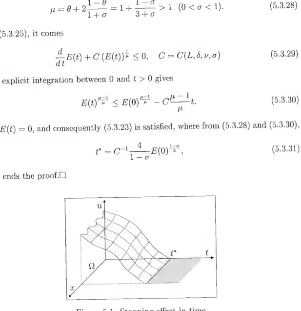
The la,st of main chapters of this thesis is Chapter 5 where the evolutionary Navier- Stokes equations are considered. The results presented in this chapter do not answer completely to ali the questions we would like. In fact vve are still vvorking on this problem. Nevertheless, many results on existence and uniqueness of a weak solution, as well the localization effect in time are already possible to show. We present these results either in their complete rigorous form, the case of localization eíFects in time, or just as simple statements, the case of existence and uniqueness of a weak solution, whose proofs are addressed to the article in preparaiion by Antontsev et ai |1 1|- I hr problem is presented in Section 5.1 and in Section 5.2 is given its weak formulai ion. In Section 5.3 severa! localization effects in time for planar bounded or unbounded domains are proved. The last section, Section 5.4, deals with the Cauchy problem, where, under certain conditions, some localizations effects in time are also proved.
In Chapter 6 we point out the resemblance between our results and some possible applications. During our research, we have found in the Hterature, or have just heard from some people working in the applications, as Professors J.I. Diaz, \ . Kalantaiov, A.V. Kazhikov and J.L. Vasquez, that our results could be applied in some situations of physical interest. In this chapter we make an attempt to use our results towards the ap- plications in Classical Elasticity in Section 6.1, Magneto-Hydrodynamics in Section 6.2 and Quasi-Geostrophic Flows in Section 6.3.
The last chapter, Chapter 7, is dedicated to the conclusions of our work that, at this moment, can be made. Rather than concluding anything, we put many questions that have arisen to us during this work. We also point out some work which we aie developing at the moment and others queries that we would like to answer positively. Of course there are also many questions the reader can pose and we would be glad and gratefnl if the reader address them to us.
Many of the results of this thesis were presented in severa! seminars given by the author at University of Algarve, University of Beira Interior, University of Évora, Technical Superior Institute at Technical University of Lisbon, Complutense University of Madrid and in the scope of the project "Nonlinear Partia! Differential Equations and Free Boundary Problems". The author has also presented Communications of some of these results in the International Congress "Navier-Stokes Equations and Related Topics (NSECcS)" hei d in 2002 at St. Petersburg, Rússia, in the "Winter School on NonLinear Partia! Differential Equations" held in 2003 at Technical Superior Institute, Lisbon, and in the International Conference "Nonlinear Partia! Differential Equations held in 2003 at Alushta, Ukraine. From these Communications and others the abstracts [6, 13, 14] were published. Article |7| was also published and articles |8, 9, 10| were accepted for publication and will appear as soon as these Journal and proceedings can it.
Faro, January 2004.
Hermenegildo Borges de Oliveira.
Contents
Resumo e Palavras-chave
Abstract and Keywords V11
XI Acknowledgements Preface X111 1 Introduction 1 1.1 Preliminaries /? 1.2 Localization EfFects 1.3 Energy Methods * 1.4 Navier-Stokes Equations ^
2 Stationary Stokes Problem 19
2.1 Introduction 2.2 Statement of the Problem ^0
22 2.3 Motivation 2.4 Weak Formulation ^ 2.5 Stopping Effect ^ 2.6 Stagnation Effect ^ 2.7 Generalizations ^
3 Stationary Navier-Stokes Problem 45
3.1 Introduction ^ 3.2 Weak Formulation 3.3 Localization Effects ^ 3.4 Appendix ^ 4 Stationary Boussinesq Problem
4.1 Introduction ^ 4.2 Statement of the Problem ^ 4.3 Weak Formulation 4.4 Localization Effects ^ 4.5 Case of a Temperature Depending Viscosity 68 4.6 Exponential Decay for the Temperature 69
5 Evolutionary Navier-Stokes Problem 71 5.1 Introduction 72 5.2 Weak Formulation 73 5.3 Localization Effects 76 5.4 The Cauchy Problem 79 6 Applications to Other Continuum Mechanics Models 83 6.1 Classical Elasticity 84 6.2 Magneto-Hydrodynamics 85 6.3 Quasi-Geostrophic Elows 86 7 Conclusions 94 Appendix 95 A. Notation 95 B. Function Spaces 98 Bibliography 401 xviii
List of Figures
1.1 Localization effect in time 1.2 Localization effect in space 2.1 Stopping effect. . . . 2.2 Dissipative forces field
2.3 Non-constant semi-iníinite strip 2.4 Stagnation effect. .
2.5 Localized forces field 5.1 Stopping effect in time 7.1 Horizontal streamlines 7.2 Circular streamlines
Chapter 1
Introduction
In this chapter we introduce the subjects which will be the aim of our work. Section 1.1 is devoted to review some results that will be used in the sequei. The presentation refers to the main bibliography we have used. In Section 1.2 we define the localization effects which will be studied in this work. Here, we give also the two main methods available to carry out this study: super and subsolutions method and energy methods. The presentation is essentially based in the monographs by Antontsev et al |12|, Diaz |34] and ÈVsgoVc |42|. In Section 1.3 a specific energy method which will be used in the forthcoming chapters to obtain the desired localization effects is described. Besides the bibliography cited in this section, we must mention the monograph by Galdi and Ri- onero |52| which we also have read. Navier-Stokes equations are derived in Section 1.4 from the principies of conservation of mass, linear momentum and energy. This deriva- tion is made in the language of modern Continuum Mechanics and, therefore, we need to distinguish Newtonian from non-Newtonian fluids. Besides the bibliography cited in this section, many other sources have been seen. We would like only to mention the monographs by Antontsev et al |15], Feistauer [45|, Galdi |49l, Kane and Sternheim 165], Kundu |71|, and the survey by Temam |116|.
2 CHAPTER 1. INTROD UCTION
1.1 Preliminaries
"The maximum principie is an important feature of second order elliptic equations that distinguish them from equations of higher order and systems of equations. "
D. Gilbarg and N.S. Trudinger |55, p. 32).
In this section, we recall some known results that will be used in the sequei. These re- sults extend from elementary inequalities to more deep results from Functional Analysis and Measure Theory.
For every a, ò > 0 and a, /? > 0, the following algehraic inequality holds
aQ^<(a + 6)^. (l.i.l)
The Cauchy-Schwarz inequality
|x-y| < |x| |y| holds for every x, y G
The Young inequality
ab<-iear^U^\\ - + 3 = 1 p P' \£J P P'
holds for every a, ò > 0, s > 0 and 1 < p < 00. If we take £ = then we obtain the equivalent Young inequality ab < 6ap + C{e) tf', with C(e) = l/[[epYFor
p = 2, this inequality is called the Cauchy inequality.
Let Í2 be a subdomain of RA with a Lipshitz compact boundary dPl. Then, the
Gauss-Green Theorem asserts that the unit outward normal n exists almost everywhere on dQ and
/ uXidx= / uriids, i =
Jn Jaó.
for every u G H1(Í2). In consequence the integration-by-parts formula
/ uXivdx= / uvnids- uvXidx, i = l,...,N,
dn Jan Jçi
is valid for every u, v e H1^). Moreover, the Green formula
uAvdK= / uS/v - nds — / Vw-VTdx dn Jdci d aa
holds for every u G H^Q) and v G H2(rí).
^If p > 1, r 1 and F{x) is defined by F{x) = f* f{t) dt for r > 1 and F{x) = íx fY) & for r < lj with f(x) > 0, then the Hardy inequality
1.1. PRELIMINARIES 3
holds, unless / = 0. The constant is the best possible and if p = 1, the two sides of (1.1.2) are equal (cf. Hardy et al |60, Theorem 330)).
Let £7 be a subdomain of and assume 1 < p <■ oo. Then the Hõlder inequality
f Máx< i + - = i,
Jn PP holds for every u G 1/(^7) and v Eljp (Í7).
Let Í7 be a subdomain of bounded at least in one direction. Assume 1 < p < oo, then the Poincaré inequality1
í \u\p dx < C í lVn|pdx, C = C(p, |Í7|), (1.1.3)
Jn Jçi
holds for every u G Wo'p(í7), and, if f7 is unbounded, ]f7| stands for the maximum
width of Í7 in the bounded direction (cf. Gilbarg and Trudinger |55)).
In this work we will appeal on many occasions to the Weak Maximum Principie. For many purposes it suffices to have the Classical Weak Maximum Principie. But, here, we consider its natural extension to operators in divergence form and for tunctions in the Sobolev space H1^).
Theorem (Weak Maximum Principie) Let us consider the following second order linear elliptic2 operator having its principal part in divergence form
L{u) = div(aVu + hu) + c • Vií + du, (1--1.4) whose coefficientsa. (matrix), b, c (vectors) and d (scalar) are assumed to be measurable in a domain Í7 o/M^. If u E H1(Í7) satisfies L{u) > 0 Oj in Í7, then
sup u < sup u+ (resp. inf w > inf ) .
o ao ^ o ao /
Notice that for the classical weak maximum principie, the condition it is imposed that the coefficient of u (in this case, div h d) is non-positive. But since the derivatives divb need not exist as functions, the non-positivity of divb + d must be interpreted in a generalized sense, i. e.
(div b + d)v dx < 0, for every v G Cj(í7).
Since b and d are bounded, this inequality will continue to hold for ali non-negative u in Wj'1^) (cf. Gilbarg and Trudinger |55|).
1This is a weaker form of a Sobolev inequality and the true Poincaré inequality corresponds to the
case p = 2. There are also some authors that, in the case of p = 2, refer to this inequality as the Friedrichs inequality (see e.g. Necas [90]).
2Ellipticity means that the coefficient matrix a is positive definite in the domain of the respective
arguments.
4 CHAPTER 1. INTRODUCTION
Strongly related with the Weak Maximum Principie is the next result we present, usually denoted as the Comparison Principie.
Theorem (Comparison Principie) Let uu u2 G H^Q) satisfy L(ui) > L^) in Q
and corresponding to houndary conditions hi and /is, respectively. If hi < h2 on díl;
then Ui < U2 in PL.
The next result gives us suitable interpolation inequalities whose applications are of the utmost importance in this thesis. Here, we have considered the original references by Gagliardo [48] and Nirenberg [91|.
Theorem (Gagliardo-Nirenberg) Assume Pl C RN and let j, k,leZ with 0<j<
k, k > 1 and l < q, r < oo. (i) If Pl is unbounded, then
where 6 is given by
P = N + e{l~'If)+(1~e)l' foral1
and C = C{j, k,N,p, q, r, 9). (ii) If Pl is bounded, then
IJlTií||lp(^) < Ci ||D^||L,(f2) 11^11^(0) + Cs |h||L9-(íí), for any q > O, (1.1.6)
where C* = Ci{j,k, N,p,q,r,9,Pl), i = 1,2. We remark that (1.1.5) and (1.1.6) only make sense if its right-hand sides are finite.
The following two results give us imbeddings of Sobolev spaces. Here, we have followed Adams |1]. The íirst one, is the so-called Sobolev Imbedding Theorem.
Theorem (Sobolev) Let Pl be a domain in having the cone property* and let Plk
be the k-dimensional domain obtained by intersecting Pl with a k-dimensional plane in with 1 < A: < TV. Let j, m be non-negative integers and let 1 <p < oo.
PART I. If mp < N, the following imbedding holds:
W^(íl)W^(^) if N — mp < k < N and p < q < kp/{N - mp). PART II. If mp = N, then the following imbedding holds:
W+rn*{Pl)-+W*(Plk) if p<q<oo.
A domain Çt has the cone property, if each point of Q is the vertex of a finite cone contained in Pl along with its closure.
1.1. PRELIMINARIES õ
PART III. If mp > N, then the following imbedding holds: W+rn'p(n) cj{n).
IfÇl is an arbitrary domain inMN, these imbeddings hold providedW:'+rn'p{Çl) is replaced
ày Wj+m,p(rí). Moreover, ifllk has finite volume, the imbeddings of Parts I and II also
hold for l < q < P-
The second result is also related to Sobolev, and is usually called the Sobolev Com- pact Imbedding Theorem. Bui contrary to the theorem name, the imbeddings in these theorems are due to F. Rellich (case p = 2) and V. Kondrachov (arbitrary p).
Theorem (Rellich-Kondrachov) Let Pt be a domain in RN having the cone property,
fio o bounded subdomain o/fi and fip the intersection o/fio with a k-dimensional plane in RN. Let m € Z such that j >0, m>l and let 1 < p < oo.
PART I. Ij mp < N, then the following imbeddings are compact:
Wj+m'p(fi) W^^fio) if 0 < N — mp < k < N and l < q < kp/{N - mp)-,
WJ+m'p(fi) -> WJ>9(fiS) if N = mp, 1 < k < N and 1 < g < oo.
PART II. If mp > N, then the following imbeddings are compact:
WJ+m'p(fi) CjiTr0) and Wj+m'p(fi) -> W^^fiJ) if l<q <oo.
IfPl is an arbitrary domain in RN, these imbeddings are compact provided WJ+m'p(fi)
is replaced by W^+rn'p(fi).
Now, we recall some results about fixed point theorems, where we have followed Gilbarg and Trudinger [55|.
Theorem (Schauder) Let A be a compact convex set in a Banach space B and let T be a continuous mapping of A into itself. Then T has a fixed point, that is, T x = x for some rc € B.
Theorem (Leray-Schauder) Let B be a Banach space and let T be a compact map- ping4 ofBx [0,1] into B such that T{x, 0) = 0 for ali x e B. Suppose there exists a
constant M such that ||x||b < M for ali {x, A) G B x [0,1] satisfying x = T{x, A). Then the mapping Ti o/B into itself given by Ti(x) = T{x, 1) has a fixed point.
The final part of this section is devoted to some results from Measure Theory. For these results, we have followed Dunford and Schwartz [40], but restrict ourselves to the case of Lebesgue measure spaces.
4 A continuous linear mapping between two Banach spaces is called compact or completely contin-
6 CHAPTER 1. INTRODUCTION
Theorem (Vitali) Let 1 < p < co and fn be a sequence of functions in I/^) con-
verging almost everywhere to a function f. Then f is in 1/(0) and
l/n - /ÍLP(fi) "*0 as ri cc
if and only if
lim / \fn{x)\p dx = 0 uniformly in n
\E\-*0JE
and for each £ > 0, there is a set Ee G O such that |Ee| < oo and such that
Í \fnix)\pdx < £, n=l, 2,
Jn\Ee
Theorem (Lebesgue) Let l < p < oo and fn he a sequence of functions in 1/(0)
converging almost everywhere to a function f. Suppose that there exists a function g in 1/(0) such that |/n(^)| < |p(^)| almost everywhere. Then f is in 1/(0) and
í fn(x) dx = í f{x) dx.
Lemma (Fatou) Let fn be a sequence of non-negative measurable, but not necessarily
integrable, functions. Then
/ lim inf fn{x) dx < lim inf / fn(x) dx.
1.2. LOCALIZATION EFFECTS <
1.2 Localization Effects
"Qualitative methods in mathematics are meihods which make it possible in absence of a quantitative solution of a mathematical problern to indicate a number of qualitative properties of the desired solution. "
L.È. Èrsgorc |42, p. vii|.
Quantitative physical laws are idealizations of reality and, as knowledge grows, we ob- serve that a given physical situation can be idealized mathematically in a number of different ways. It is therefore important to characterize those reasonable ideal formula- tions. Hadamard |59| asserts that a given problem for a partial differential equation is wcll-poscd, if the problem in fact has a solution, this solution is unique and it depeneis continuously on the data given in the problem. These criteria are reasonable from the Physics point of view in most cases. Existence and uniqueness are an affirmat ion oí the Principie of Determinism5, without which experiments could not be repeated with the
expectation of consistent data. The continuous dependence criteria is an expression of the stability of the solution, i.e., a small change in any of the problem data should produce only a correspondingly small change in the solution. These criteria are usually referred as the qualitative properties of the problem in contrast with the quantitative properties which mainly concern with finding an exact solution or, at least, an approx- imated one. Sometimes the qualitative analysis of a mathematical problem is only the first step of an investigation, in which one proves the existence, estimates the num- ber of solutions and establishes some peculiarities of the solutions, thus facilitating in the future their exact or approximated solution. However, one frequently has to deal with problems in which the question is, from the beginning, purely qualitative and the finding of an exact or approximated solution does not make it possible to answer the question as posed and frequently does not even help in finding the solution of that problem.
The main goal of this thesis is the study of some qualitative properties of the solu- tions of some problems arising in Fluid Mechanics and which are known in the literature bv the widened name of localization effects. Roughly speaking, the localization effects are ali the properties which one can prove to localize the solutions in some part of the problem domain. Localized solutions occur when the influence of the data, such as initial conditions, boundary conditions and or prescribed functions, on the behavior of solutions is restricted to the points of the domain close enough to the support of the data. The localization effects depend on the nature of the problem, specifically if it is of stationary or evolutionary type. If the problem is of stationary type, the localization effect can only be studied on the space and if it occurs, we say, solely, we have a localized solution.
5 Determinism is the philosophical doctrine that claims that ali behavior results from preceding
events or natural causes. Scientific determinism makes a very strong assertion, that ali events are in principie predictable (see e.g. Popper |95|).
8 CHAPTER 1. INTROD UCTION
Definition 1.2.1 Let Q be an open subset r;/and let u : Pi —> R 6e a solution, at least in a weak sense, of a yiven stationary boundary-value problem in Pi. We say that u is a localized solution if it vanishes in an open subset of Q.
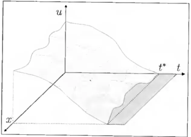
When the problem is of evolutionary type, there are two main different localization effects. localization in time and localization in space. The localization effect in time corresponds to the stabilization oí solutions in a finite time to a stationary state. Definition 1.2.2 Let Pi be an open subset ofRN, 0 < T < oo and u : Px (O.T) R a
solution, at least in a weak sense, of a yiven initial boundary-value problem in Pix (0, T). We say that u(x,t) stabilizes in a finite time to a stationary state us, if there exists
t* e (0, T) such that for ali t G [t*, T), u(x, t) = us(x) in P.
If the stationary state is zero, we say that there is an extinction in a finite time. Most results in the literature of stabilization in a finite time to a stationary state concern the case of extinction in a finite time.
Among the piopeities of stabilization in a finite time, one can find the finite speed of propagations and the formation of dead cores. Both are related to a degeneration introduced in the problem when the solution attains certain s-level, usually normalized to be zero. Finite speed of propayations means that the speed of propagations of distuibances from the initial data is finite. In other words we can talk about finite speed of propagations, if solutions corresponding to compact supported initial datum remain with compact support, at least for some time. Dead core means that, even if the initial datum is strictly positive, a region where the zero levei is attained may appear in finite time. In mathematical terrns this means that there exists > 0 such that RN \ {supp u.(., í)} ^ 0 for ali t > t*, in spite of suppw0 = R^. Even in stationary
problems, one can talk about the dead core formation in the case where the solution vanishes in an interior region.
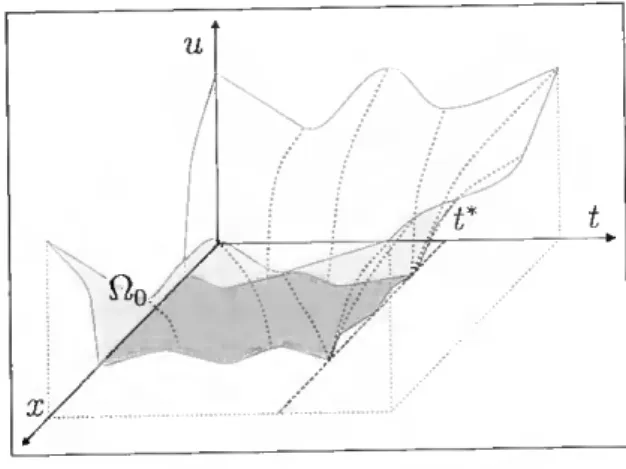
The localization effect in space corresponds to the stabilization of solutions in some space subdomain and in some interval of time.
u
1.2. LOCALIZATION EFFECTS J
Definition 1.2.3 Let El be an open subset ofRN, 0 < T < oo and u : ílx (0,T) ^ R a
solution, at least in a weak sense, of a given initial houndary-value problem in Q x (0, T). We say that u{x, t) has the property of localization in space, if there exists an open subset í2o ofEl and U € ((),T] such that u{x,t) = 0 a.e. in Elo and for ali 0 <t <U.
For the sake of simplicity, we have introduced the concept of localization in space to the zero-levei of u{x,t). But, considering the function u{x,t) - s with s ^ 0, we can extend this concept in a natural way with respect to the s-level. In the literature one can find two main localization effects in space: waiting time property and support shrinking property. In the special case of the right-hand side of a partia! differential equation is zero (/(M) = 0), the time U is called the waiting time and then we say the solutions satisfy the waiting time property. The solution of some initial boundary value problem has the support shrinking property, if for any t > 0 the support of solution u{x, t) is bounded, even if it is unbounded for t = 0.
We remark that the property of localization in time is global, i.e. u{x,t) vanishes in the whole 17 if í > U, in contrast with the property of localization in space which has a local character, i.e u{x,t) merely vanishes in 17o if t <U. A special class of locahzed solutions corresponds to the case when the domain is unbounded and the supports of solutions are bounded and therefore compact.
From the mathematical point of view, ali these localization effects mean that the set suppw is strictly contained in the problem domain. A physical meaning for this situation can be interpreted as the dissipation oí the quantity under study (density, concentration, temperature, velocity, etc.) in some part oí the domain. A good sur- vey for applications of the localization effects to problems in Fluid Mechanics is the monograph by Antontsev et al |12|.
In order to carry out the study of the localization properties, two main general methods are available: the super and subolutions method and the energy methods. The first method is based on the construction of adequate super and subsolutions u and u to which, jointly with the solution u of the considered partial differential equation, the Comparison Principie is applied. Such functions can be chosen with compact support and so, by a comparison argument, u < u < ú \\\ the considered domain 17, which implies that suppu is also a compact subset. Due to the use of Comparison Principie,
u
10 CHAPTER 1. INTROD UCTION
this method is especially useful in the study of second and also first order equations. Although the Comparison Principie implies automatically the uniqueness of solution, this method can also be applied to some monotone problems and systems in which the uniqueness fails. The idea for using super and subsolutions to establish the localization effects is quite classical in the theory of partial differential equations and, for nonlinear problems, such functions are taken locally as suitable interior or boundary barriers functions. The use of Comparison Principie, and to the best of our knowledge, goes back to the work of Oleinik et al |92| on a degenerate parabolic equation.
The energy methods rely on the idea of finding some ordinary differential inequal- ities satisfied by some energy functions involving the integral, over some subsets, of some suitable chosen differential expressions of the solutions. These methods will be the scope of the next section.
An important question connected with the localization effects, is the free boundary. also called the interface, generated by the unknown boundary of the support of the solutions. For instance, the function
r \ p/(p-g-i) u(x) = Uo(l- — j where sp - 7í(P-9-1)/P Xo — U0 V (P - 1)^ i/p (1.2.7) (1.2.8) p-q-l
is a solution of the following one-dimensional free-boundary problem: to find a non- negative function u(x) and a positive íinite number Xq such that u satisfies
Lu= {\ux\p 2ux) + \u\q lu = 0, q<p-l, (1.2.9)
in (0,3:o) and
u(0) = u0, u{xo) = 0, MxoFM^o) = 0-
On the other hand, the function ^(3:) given above in (1.2.7)-(1.2.8) is a localized solution of equation (1.2.9) in the domain = (0,00) and observe that supp u = (0,xo). In this vvay, by a free boundary, we mean a curve separating the regions where the solution vanishes (or stabilizes at a s-level) or it is positive (see Antontsev et al |12| and Diaz |34|).
1.3. ENERGY METIIODS 11
1.3 Energy Methods
"A/l of the methods which lead to variai i ou ai problems for hounded func- tionals can be considered energiy methods in a generalized sen,se."
D.D. Joseph |63, p. 3|.
By energy method one denotes a snitable mathematical device for deriving estimates of solutions to differential equations. The name of the method is due to the fact that it is usually founded upon conservation and balance laws from continuum mechan- ics and which must be satisfied by the solutions. A typical example of an energy method, and to our knowledge the first one, is given by the approach introduced by Lyapunov [83] for studying the stability of solutions to ordinary differential equations. Although found the works of Lyapunov on what we call nowadays energy methods, this mathematical device only became known with the works of Friedrichs |4( | in Partial Differential Equations to establish existence and uniqueness results and to prove the convergence of some difference schemes. In Flui d Mechanics the energy method was introduced by Serrin [104] in a way which consists in forming the kinetic energy of per- turbations to a given basic ílow and in studying its behavior in time. This method was successively generalized and enlarged by Joseph and his co-workers [63] foi studying nonlinear stability of viscous incompressible flows in hounded domains. Still in Fluid Mechanics, Straughan [112] has developed the energy method in a variety of contexts: half-space problems, geophysical problems, convection driven by surface tension, con- vection in other classes of íluids, tim^dependent convection problems and lias studied the connection with the there-called Lyapunov method in partial differential equations. The main goal of this thesis is to study some qualitative properties of problems arising in Fluid Mechanics by using a specific energy method which is denoted by energy method for free boundary problems (cf. Antontsev et ai [12]). Energy methods are of special interest in those situations in which traditional methods based on the Comparison Principie have failed. A typical example of such a situation is either a higher-order equation or a system of partial differential equations. We note that energy methods are well suited in the study of partial differential equations systems which include equations of different types frequently arising in the mathematical models of continuum mechanics. In such systems, the various unknowns (velocity, density, saturation, e/c.) may satisfy equations of different types and need not even be defined on the same domain. Moreover, even when the ( omparison Principie holds, it may be extremely difficult to construct snitable sub or super-solutions if, for instance, the equation under study contains transport terms and has either variable or unbounded coefficients or the right-hand side. The main idea of the energy methods consists in deriving and studding snitable ordinary differential inequalities for various types of energy. In typical situations, these inequalities follow from the conservation and balance laws of Continuum Mechanics. In the simplest situation, the energy functions defined through a formal procedure coincide with the kinetic and potential energy.
The here so-called energy method for free boundary problems was introduced by Antontsev [5] in order to prove that, for general multidimensional degenerate parabolic
12 CHAPTER I. INTRODUCTION
equations, the finite speed of propagation of disturbances from initial data is finito and that. for degenerate elliptic equations, the solutions defined in domains infinito in extent with respect to one of the variables vanish on a set of positive moasure. A moro systematic treatment of this topic was made by Diaz and Veron |38, 39|. This method was onlarged by many authors, amongst whom Bornis [18. 211 gavc the general treatment for higher-order elliptic and parabolic equations. A difforont approach to establish several localization effects for quasi-Iinoar parabolic equations was given by Shishkov [107, 108] by using a slightly difforont enorgy method. Roughly speaking. the enorgy method for free boundary problems consists in three stops. The first is to multiply the partia! differential equation by a weak solution and to intograte by parts over a variable or moving subdomain. This leads to enorgy integrais plus other torms over the boundary of the subdomain. Sometimes it is useful also to multiply the partia! difforontial equation by a weight which will cancel some boundary torms. In almost ali cases it is considered a variable bali or a variable half-space. The choico of integrating over a bali or a half-space is related with the nature of the problom under considoration. VVhen using balis, the boundary conditions may not have to be zero, but it is very hard to work with when considoring higher-order equations, because of the boundary torms resulting from integrating by parts. The uso of half-spacos is easier to handlc higher- order equations, but it requiros zero Dirichlet boundary conditions. The second stop is to use interpolation-imbodding inequalities related to Sobolev imbedding inequalities. I hese two stops give us an ordinary differential inequality which is satisfiod by the natural energies associated to the problem. The independent variable of this differ- ential inequality is just the variable which labels the moving subdomain. The third stop is to doduce from the resolution of this differential inequality somo qualitativo properties, usually denoted by localization effects, of the solutions of the original prob- lem. í his method allows us to deal with a great variety of problems formulated in a very general form. where no monotonicity assumption on the nonlinearities is required, the Comparison Principie is not invoked and no restriction on the space dimension is required.
A common fact among the different enorgy methods that can be used, is the rcduc- tion, sometimes by means of quite sophisticated techniques, to some ordinary differ- ential inequality satisfied by the energy function. This inequality is very dose to the following problem6
+ a(t)V(h(t)) = 0. h{0) = ho>0. (1,3.10)
Once we assume
fT ds
^(r) = / —— < oo, for every r > 0 and ^ > 0, ./u W)
"Due to the relevance of the equation appearing in (1.3.10), Diaz [36] proposes to call this type of equations as the Torricelli-Bernoulli equations in honor of Evangelista Torricelli (1608-1647) vvho proposed the related law v = v/2///) for the study of the efflux of a liquid from a small orifice in the wallsof a vessel, and Daniel Bernoulli (1700-1782) who proved that —dh{f)/(H = r2/R2y/2gh, where
v — —dh(t)/dt is the velocity at the bottom, r and R are the radium of the circular sections at the bottom and at the top, respectively, and // is the gravitaiional acceleration.
1.3. ENERGY METHODS 13
a > O and a € 1^(0, oo), the solution is given by
h{t) = ^ y{h0) - a(r) dr
and, in particular, if
To
V{h0) - í a{r) dr = 0 for some Tq > 0,
Jo
which is certainly the case if afr) dr —>• oo as í —> oo, then 3 Tq > 0 ; h{t) = 0 V í > Tq.
This extinction property also holds for solutions of the inequality ^M + a(íM/i(í)) <0,
dt
since the Comparison Principie applies in the class of non-negative solutions.
We notice that such problems as (1.3.10) are also relevant in the application of other kinds of methods as the super and subsolutions method (cf. Diaz |34]).
14 CHAPTER 1. INTROD UCTION
1.4 Navier-Stokes Equations
"Such models were not new, having occurred in philosophical or qualitative speculations for millennia past. Navier 's magnificent achievement was to put these notions in concrete form that he could derive equations of motion for them. "
C. Truesdell |118, p. 455].
Navier-Stokes equations were proposed in 1822 by Navier [89] on the basis of suitable molecular models. The first mathematical description of the motion of an (ideal) fluid was formulated by Euler [43] in 1755 as a statement of the Newton's second law of motion1 applied to a fluid moving under an internai force known as the pressure gra-
dient. Navier's great achievement was to include in the Euler equations the effects of attraction and repulsion between neighboring molecules. These equations were red- erived by Cauchy [32] in 1828, by Poisson [94] in 1829 and in 1843 Saint-Venant [99] published a derivation of the equations on a more physical basis applied, not only to the so-called laminar flows, but also to turbulent flows. However, it was only in 1845 that, by the clarifying work of Stokes [111], these equations found a completely satisfactory justification on the basis of the continuum mechanics approach.
We recall briefly the derivation of Navier-Stokes equations in the language of the modern continuum mechanics. We consider the motion of a fluid that occupies at time t a domain of the space R3. For the sake of simplicity, we assume that flt = Çl is
independent of time, since the mathematical difficulties for moving domains tend to hide difficulties specific of the Navier-Stokes equations. In continuum mechanics, the Lagrangian representation of the motion consists in providing the trajectory of each particle of fluid, x = <I>(a, í), where a = (a, 6, c) is the position at time 0 of the particle of fluid, x = (x,y,z) its position at time t. Navier-Stokes equations in their most common form correspond to the Eulerian representation of the flow, which provides the vector fields u = {u, v, w) corresponding to the velocity of the particle of the fluid which is at x at instant t. We have
c)ã>
u(x,í) = -^(a,í),
and conversely we can recover the Lagrangian representation of the motion from the Eulerian one by solving the systems of ordinary differential equations
dxa(í)
—= u(x, í), xa(0) = a (xa(í) = ^(a, t)).
Equations describing fluid flow are derived on the basis of three fundamental physical principies (cf. Serrin [104]).
Principie (Conservation of Mass) The mass of fluid in a material volume uj does not change as w moves with the fluid.
1.4. NAVIER-STOKES EQUATIONS 15
Principie (Conservation of Linear Momentum) The rate of change of linear momentum of a material volume cu equals the resultant force on the volume.
Principie (Conservation of Energy) The rate of change of total energy of a material volume is equal to the rate at which work is being done on the volume plus the rate at which heat is conducted into the volume.
The continuity equation which expresses the Principie of Conservation of Mass, reads
+ pdivu = ^ 4-div (pu) = 0. (1.4.11) dt ot
The equation of motion which expresses the Principie of Conservation of Linear Momentum, reads
du
— + (u. V)u ^f + divS, (1.4.12)
where p = p(x, <) is the density, 7 = 7(x, í) is the acceleration, f = f(x, t) represents externai volume forces applied to the fluid and S is the (Cauchy) stress tensor. In this thesis we use the commonly accepted definition for a fluid as a Stokesian fluid, i.e., an isotropic continuous médium such that S is a continuous function of the rate of strain tensor
D = -(Vu + VUt), (1.4.13)
S = f(D), and, when D = 0, S reduces to -pl, the case on an ideal fluid, where p = p(x, t) is the pressure of the fluid, and I is the unit matrix. The isotropy condition is expressed by QSQ"1 = f (QDQ-1) for ali orthogonal transformations matrices Q,
which means that there is no preferred direction either in the fluid or in space. For a fluid defined like that, one can prove, from (1.4.12), the following principie holds (cf. Serrin [104|).
Principie (Conservation of Angular Momentum) The rate of change of angular momentum of a material volume uj equals the angular momentum of the resultant force on the volume.
As a consequence of the Principie of Conservation of Angular Momentum, the stress tensor S is symmetric.
The energy equation which expresses the Principie of Conservation of Energy, reads
+ pedivu = + div(peu) = S : D - divq, (1.4.14) dt ot
where e is the specific internai energy per unit mass and q is the rate of heat transported by conduction, usually denoted by heat flux8. Occasionally a term (pg, g is the heat
producing capacity) is added to the right-hand side of (1.4.14) to account for various
8It is more usual to call —q the heat flux, since q - n < 0 at points where heat is entering the body
16 CHAPTER 1. INTRODUCTION
other types of energy sources in the fluid, such as those resulting from chemical reaction, radiation, etc. Here, we follow the commonly accepted formulation and postulate that q is an isotropic function of the temperature and thermodynamic state and thus must be parallel to Ví?. Whence follows the Fourier law
q=-fcV0, (1.4.15) where 6 is the absolute temperature and /c > 0 is a scalar function called thermal conductivity, which in most cases, is taken to be simply a function of p, V and |V9|, or even a constant called the thermal conductivity coefficient. Hence (1.4.14) becomes
d" pedivu = —+ div(peu) = S : D + div {kVO). (1.4.16) According to the Reiner-Rivlin principie of material objectivity, the stress tensor in its most general form is given by
S = —"pi + 0ol + 0iD + (1.4.17) where (/>i, z = 0,1, 2, are given scalar functions of the principal invariants of the rate of strain tensor D (cf. Truesdell and Noli [119]).
For the so-called Newtonian fluids, such as liquids and gases, (po = A ii, (pi = 2/i, (p2 = 0 and the stress tensor obeys the Stokes law
S = —pi-f Adivul + 2pD, (1.4.18) where p is called the shear viscosity and A the hulk viscosity. In many cases p and A are constants and, in that case, they are called the first and the second coefficient of viscosity, respectively. Replacing the stress tensor (1.4.18) in (1.4.12) and (1.4.16), we obtain
P and
^ + V(pe) • u = -pdivu + A(divu)2 + 2p |D|2 + div {kV6). (1.4.20)
The set of equations constituted by (1.4.11), (1.4.19) and (1.4.20) is not closed and in order to close it, it remains to describe p, p, e and 0. If we choose as independent variables p and 6, then p and e are functions of p and 9, i.e., obey some given state equations of the following form
P = P(P,0), e = e(p,0). (1.4.21) Therefore it is necessary to introduce some supplementary information of thermody- namics (cf. Batchelor [16]).
1.4. NAVIER-STOKES EQUATIONS 17
First Law of Thermodynamics The entropy9 s of a system is given by 9ds —
de + pd{l/p).
Second Law of Thermodynamics For any process, the total entropy of a system plus its surroundings may never decrease.
A consequence of the Second Law of Thermodynamics asserts that > 0 and 3A + 2// > 0. Equations (1.4.11), (1.4.19), (1.4.20) and state equations as (1.4.21) constitute the general set of equations upon which classical hydrodynamics is based.
At this point we need to define an important intrinsic characteristic of some fluids. If the volume of any part of the fluid remains constant during the motion, we say the fluid is incompressihle, which is expressed by
divu = 0. (1.4.22) In this case, (1.4.19) and (1.4.20) can be simplified by eliminating terms containing div u,
- Vp + div (2pD) (1.4.23) and
+ V(pe) • u = 2/i |D|2 + div [kVe]. (1.4.24)
ot
In this case, p is the mechanical pressure, a fundamental dynamical variable, and p is a scalar function of the temperature satisfying p > 0. The energy equation (1.4.24) is separated from the system {(1.4.22), (1.4.11), (1.4.23), (1.4.24)} and is solved after the velocity and pressure are found.
Fluids which do not exhibit property (1.4.22), such as gases, are denoted compress- ible fluids. For such fluids p is the thermodynamic pressure and p and A are scalar functions of the thermodynamic state.
If the fluid flow is isothermic, i.e., 9 is constant, then energy equations (1.4.20) and (1.4.24) are usefulness. In this case, {(1.4.11), (1.4.19)} is usually denoted by the com- pressible Navier-Stokes system and {(1.4.22), (1.4.11), (1.4.23)} by the incompressible Navier-Stokes system.
For non-Newtonian fluids, the stress tensor is given by
S = —pi + F(D, p, 9), (1.4.25) where F is a nonlinear function of D. Examples of such fluids are suspensions and high molecular-weight materiais. Several constitutive relations have been suggested in order to capture characteristics of non-Newtonian fluids (cf. Showalter [109], Truesdell and Noli [119)), but we will not study fluids with such behavior here. Interesting situations are those for incompressible fluids when it is assumed that
(fi ^ const. and = 0. (1.4.26) du
dt -I- (u - V)u
18 CHAPTER 1. INTRODUCTION
Some authors call fluids satisfying these conditions purely non-Newtonian (cf. Antont- sev et al [12|) and others call them generalized Newtonian fluids (cf. Showalter [109]). A subclass of such fluids is constituted by the Ostwald-de Waele fluids, also called power type fluids, for which
4*1 = 2(/z H- t |D|q—1), for some r > 0 and q > 0, (1.4.27)
with |D| = D : D. The fluid is called dilatant or viscous-plastic if q > 1 and pseudo- plastic if 0 < q < 1. If q = 1, we revert into the class of Newtonian fluids.
Now, we restrict ourselves to the case of incompressible (Newtonian) fluids. In this case, the continuity equation (1.4.11) implies the density p is constant along the trajectories of the fluid. Hence, if the fluid is homogeneous, p(x, 0) = po > 0 is independent of x. Then, we can divide (1.4.23) and (1.4.24) by po to obtain
d\x
— + (u • V)u = f - Vp-f div (2i/D) (1.4.28) and
de 9
—-\-Ve-u = 2i'\D\ +div(A:V#). (1.4.29) We have set v = p/po, the kinematic viscosity, and we have renamed p/po as
m and k/po as k, where p is now called the hydrostatic pressure.
To conclude this section, we notice the equations describing fluid flows must be supplemented with boundary conditions characterizing the flow on the boundary of the domain occupied by the fluid and by initial conditions determining the initial state of the flow at the beginning of the time interval considered. The question of initial condition is immediately understood from the physical point of view, but the question of boundary conditions is much more delicate and would require a detailed discussion. Our ambition in this thesis is somewhat limited since we shall consider problems set in a domain íl, with standard mathematical boundary conditions on dfl.
Chapter 2
Stationary Stokes Problem
"As follows from experiments, the Stokes problem descrihes slow flows of very viscous fluids relatively well. Moreover, The Stokes problem is also used in iterative methods for the solution of the nonlinear Navier-Stokes equations."
M. Feistauer [45, p. 509].
This chapter is concerned with the study of the planar stationary Stokes problem. This problem is introduced in a semi-infinite strip, in Section 2.1, as a simplification of the Navier-Stokes equations presented before. The complete statement of the problem considered in this chapter is given in Section 2.2, where a result about the exponential decay for the weak solutions to the classical Stokes problem is also recalled. We give, in Section 2.3, the motivation for the forces íield type considered here by giving some known results in this direction and by showing the difficulties felt at the beginning to prove the localization effect. The complete weak formulation of the problem is presented in Section 2.4. There we prove the existence theorems for this problem and the imiqueness one as well. To prove these results, we will use some known results for the Stokes equations with prescribed linear forces field. In almost the situations the reader is addressed to the precise sections of the monograph by Galdi [49] to see the proofs of these results. But, in fact, many other sources have been seen, such as the monographs by Constantin and Foias [33], Ladyzhenskaya [72] and lemam [115]. The main result of this chapter is the localization effect which we have denoted by stopping effect and is proved in Section 2.5. This result is proved in a constructive way, being presented the auxiliary results as they are needed. In Section 2.6 we prove another localization effect which we have denoted by stagnation effect. Section 2.7 is devoted to generalize these localization effects for localized forces field.
20 CHAPTER 2. STATIONARY STOKES PROBLEM
2.1 Introduction
Let us consider the stationary Stokes system
—i/Au = f - Vp, (2.1.1) div u = 0 (2.1.2) in a semi-infinite strip like domain Í2 = (0, oo) x (0,L), L > 0 a positive constant, where í/ is the kinematic viscosity coefficient. Stokes system (2.1.1 )-(2.1.2) is derived from the Navier-Stokes system {(1.4.22), (1.4.11), (1.4.23)} by assuming the fluid is homogeneous, the kinematic viscosity is constant, the velocity and pressure do not depend explicitly on time and by a linearization procedure on the resulting stationary Navier-Stokes equation. Such a linearization is made under the mechanical assumption the fluid viscosity is large, i.e. i/ 1, and the velocity is sufficiently small. As fol- lows from the experiments, this is characteristic of slow flows and means that the ratio |(u • V)u|/|//Au| of inertial to viscous forces is vanishingly small, so that we can disre- gard the nonlinear term (u • V)u in the stationary Navier-Stokes equation. Moreover, if we assume reference length / and velocity u, this linearization amounts to assume the dimensionless Reynolds number TZ = vi/u \s suitably small. The consideration of the planar domain Q, means that we are facing a flow with only two velocity components, say u(x,y) and v(x,y). This corresponds to a number of cases where it is possible to introduce a Cartesian coordinate system {x:y,z) such that the quantities describing
the flow are nearly independent of the variable 2 and the velocity component w in the direction z is negligible. We thus obtain the model of plane flow where the domain Q C M3 occupied by the fluid has the form of a cylinder oj x (0,c), u C M2 and c > 0,
with axis orthogonal to the plane (x,y). The flow has the same character in ali planes orthogonal to the axis 2: and the velocity component w vanishes.
2.2 Statement of the Problem
We consider the Stokes system (2.1.1)-(2.1.2) to whom we append a possible non-zero velocity at the strip entrance
u(0, y) = u*(y), y G (0, L) (2.2.3) and zero velocity on the lateral wall
u(x.O) = u(x, L) = 0, x £ (0,oo). (2.2.4) Since Q is unbounded, we have to prescribe the velocity at infinity. We are interested in the case
|u(a:,í/)| —>-0, as .t -> 00 and y G (0,T). (2.2.5) We recall that due to the incompressibility condition (2.1.2), the first component of
u*(í/) — (u*{y)iv*(y)) must satisfy
í u*{s)ds = 0. (2.2.6) Jo
2.2. STATEMENT OF THE PROBLEM 21
We also assume the compatibility conditions
u*(0) = u*(L) = 0. (2.2.7) The main question we shall consider here can be stated in the following terms: can we find a vector jield f such that the weak solutions of problem (2.1.1)-(2.2.5) have compact support in Í2, i.e.,
u — 0 for every x > a:u, for some a:u > 0?
y L
u = 0
0 .7 u =? X
Figure 2.1: Stopping effect.
From the Physics point of view, this corresponds to search for a body forces field stopping the fluid at a finite distance from the strip entrance. This property cor- responds to a localization effect as stated in Section 1.2 that we will denote by the stopping effect.
It is well known the weak solutions u of problem (2.1.1)-(2.2.5) when we prescribe zero externai forces field, have an exponential decay which is optimal
||u|lHi(oa) < Cl exp(-C2a), for ali a > 0, (2.2.8)
where C*i, C2 are positive constants depending on L, ||u||Hi(fi) and zz (cf. Galdi |49, §VI.2|). This result still holds, if we consider a non-zero linear forces field, say f G L2(Q), and with compact support in tt. In these cases, the weak solutions of prob-
lem (2.1.1)-(2.2.5) do not have compact support in íl and the localization effect does not hold. One can easily adapt to this problem the exponential decay results 011 the Saint-Venant's Principie1 in the two-dimensional linear theory of elasticity obtained
separately by Toupin |117] and Knowles |68|.
The answer will be positive for a body forces field given in a feedback dissipative forni, f : íí x R2 —> R2, f = (/1, /2), such that for every u G R2, u = (u, r;), and almost
ali x G
—f(x, 11) u>ô lu|1+a — g{x.) (2.2.9)
for some constants ^>0, ()<<7<1 and some function
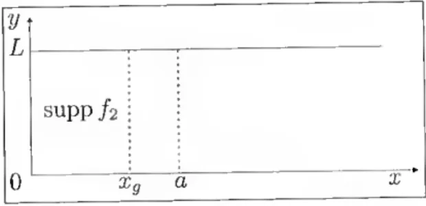
g G L1 (ÍT9), ^ > 0, (y(x) = 0 a.e. in PtXg, (2.2.10)
where ST9 = (0, Xg) x (0, L) and ÇlXg = (xg, 00) x (0, L), with 0 < < 00. The novelty
of this forces field is the dependence of f, not only on the spatial variable x, but also 'See Remark 2.5.4 on page 40.