João Rodrigues Correia Ramos
Licenciado em Biotecnologia
Analysis of Metabolic Flux Distributions in
Relation to the Extracellular Environment in Avian Cells
Dissertação para obtenção do Grau de Mestre em
Biotecnologia
Orientador:
Dr. Moritz von Stosch, investigator Post-doc, FCT-UNL
Co-orientadores: Dr. Rui M. Freitas Oliveira, Professor Associado, FCT-UNL
Júri:
Presidente: Dr. Pedro Miguel Calado Simões
Arguentes: Dra. Ana Margarida Palma Teixeira
iii
Analysis of metabolic flux distribution in relation to extracellular environment in avian cells
Copyright © João Rodrigues Correia Ramos, Faculdade de Ciências e Tecnologia, Universidade Nova de Lisboa.
vii
Acknowledgments
This leap in to an excitement future would not be possible without all the emotional and scientific support of many people who have accompanied me through these last years. This a like a dream coming true and I have many people to thank for it.
First, I would like to thank my advisor, Dr. Moritz Von Stosch, for the opportunity to work in this exciting field. I am very grateful for his encouragement, guidance and knowledge, which allowed me to fulfill my goals. Also, I am thankful to my co-advisor Dr. Rui Oliveira for all the help and insight during this work.
I would like to thank Fundação Lapa do Lobo, especially Dr. Carlos Torres, for believing in me all this time and of course for the precious scholarship that got me this far.
I am very thankful to my family and to my girlfriend, whose love and the continuous support during all these years, made all things possible in my life.
ix
xi
Abstract
Continuous cell lines that proliferate in chemically defined and simple media have been highly regarded as suitable alternatives for vaccine production. One such cell line is the AG1.CR.pIX avian cell line developed by PROBIOGEN. This cell line can be cultivated in a fully scalable suspension culture and adapted to grow in chemically defined, calf serum free, medium [1]–[5]. The medium composition and cultivation strategy are important factors for reaching high virus titers.
In this project, a series of computational methods was used to simulate the cell’s response to different environments. The study is based on the metabolic model of the central metabolism proposed in [1]. In a first step, Metabolic Flux Analysis (MFA) was used along wit h measured uptake and secretion fluxes to estimate intracellular flux values. The network and data were found to be consistent. In a second step, Flux Balance Analysis (FBA) was performed to access the cell’s biological objective. The objective that resulted in the best predicted results fit to the experimental data was the minimization of oxidative phosphorylation. Employing this objective, in the next step Flux Variability Analysis (FVA) was used to characterize the flux solution space. Furthermore, various scenarios, where a reaction deletion (elimination of the compound from the media) was simulated, were performed and the flux solution space for each scenario was calculated. Growth restrictions caused by essential and non-essential amino acids were accurately predicted. Fluxes related to the essential amino acids uptake and catabolism, the lipid synthesis and ATP production via TCA were found to be essential to exponential growth. Finally, the data gathered during the previous steps were analyzed us ing principal component analysis (PCA), in order to assess potential changes in the physiological state of the cell. Three metabolic states were found, which correspond to zero, partial and maximum biomass growth rate. Elimination of non-essential amino acids or pyruvate from the media showed no impact on the cell’s assumed normal metabolic state.
xiii
Resumo
Culturas de células contínuas, capazes de proliferar em meios simples e definidos, são vistas como possíveis alternativa para produção de vacinas. Uma tal alternativa é a linhagem celular aviaria AG1.CR.pIX, recentemente desenvolvido pela PROBIOGEN. Estas células, além de crescer em suspensão, crescem num meio simples sem derivados de animais.
Neste projeto, vários métodos computacionais foram usados para simular a resposta destas células a diferentes meios. Este estudo é baseado no modelo de metabolismo central proposto em [1]. Numa primeira abordagem, Metabolic Flux Analysis (MFA) com os fluxos de consumo e de secreção foi aplicado para estimar os fluxos intracelular. A rede e os dados revelaram ser consistentes. Numa segunda fase, Flux Balance Analysis (FBA) foi implementado para aferir o objetivo biológico das células. O objetivo para o qual foi obtido uma melhor correlação entre os fluxos previstos com os experimentais foi a minimização da fosforilação oxidativa. Usando este objetivo, Flux Variability Analysis (FVA) foi implementado para obter a variabilidade dos fluxos. Além disso, este método foi aplicado a vários cenários onde a eliminação de uma reação (equivalente a eliminação de compostos do meio) foram simulados. As restrições causadas por aminoácidos essências e não essenciais foram corretament e previstos. Os fluxos relacionados com consumo e catabolismo de aminoácidos essenciais, síntese lipídica e produção de ATP via TCA revelaram-se como essências durante o crescimento exponencial. Por fim, os dados obtidos na etapa anterior foram analisados usando o Principal Component Analysis (PCA), para aferir sobre possíveis mudanças no estado fisiológico das células. Foram encontrados três estados metabólicos, correspondentes a zero, parcial e máximo crescimento celular. A eliminação de aminoácidos não essenciais ou do piruvato do meio não mostrou nenhum impacto no estado metabólico assumido como o normal para estas células.
xv
Contents
1
Introduction ... 1
1.1
The avian cell line AG1.CR.pIX... 1
1.1.1
Background ... 1
1.1.2
The CR.pIX metabolic model... 3
1.2
Objectives ... 5
1.2.1
General objectives ... 5
1.2.2
Specific objectives ... 5
2
Methods... 7
2.1
Cell culture and sampling ... 7
2.2
Calculation of the uptake and secretion fluxes ... 7
2.2.1
Calculation of the fluxes ... 7
2.2.2
Monte Carlo Sampling for the calculation of the flux standard deviation... 9
2.3
Constraint Based Models - Methods for determination and analysis of the cellular
flux distribution ...10
2.3.1
Metabolic Flux Analysis ...10
2.3.2
Flux Balance Analysis ...12
2.3.3
Flux Variability Analysis ...14
2.3.4
Principal Component Analysis ...15
3
Results and discussion ...17
xvi
3.1.1
Exponential biomass growth phase...17
3.1.2
Substrates and metabolic products...19
3.2
Metabolic Flux Analysis ...21
3.2.1
The determined Fluxes...21
3.2.2
Estimated intracellular fluxes ...23
3.2.3
Consistency check...24
3.3
Flux Balance Analysis ...27
3.3.1
The cell objectives ...29
3.4
Flux Variability Analysis ...32
3.4.1
Flux variability for FBA results with assumed biological objective ...33
3.4.2
Flux variability with different condition environment simulation ...35
3.4.1
The glutamine free medium flux variability ...37
3.5
Principal Component Analysis...38
3.5.1
Number of components ...39
3.5.2
Metabolic states ...42
3.5.3
The glutamine free medium ...45
4
Conclusion ...47
5
Future Work ...49
6
Bibliography ...51
7
Appendix ...55
xvii
List of Figures
Figure 1.1: The CR. pIX central metabolic model, adopted from Lohr et al [2] . ... 4
Figure 2.1: Example of FBA applied to a metabolic network, adapted with permission from Macmillan Publishers Ltd: Systems-biology approaches for predicting genomic evolution from [23], copyright 2011. ...14
Figure 3.1: Biomass exponential growth curve. ...18
Figure 3.2: Measurements and linear regression model of the biomass concentration in logarithmic scale over time for the exponential growth phase. ...19
Figure 3.3: Typical variations in substrate uptake and metabolic product formation for CR.pIX cells cultivation. Black line: interpolation. A: extracellular concentration of glutamine (■) and ammonia (♦). B: extracellular concentration of glucose (▲) and lactate (▼). C: extracellular concentration of serine (●) and glycine (◄)...20
Figure 3.4: Metabolic flux distribution in pIX. ...23
Figure 3.5: Consistency check results: h-value over time. Test hypostasis X2(0.95, 2) ( ̶ ). ...25
Figure 3.6: Mean of the coefficient of contribution for each of experimentally measured compounds on the model consistency. ...26
Figure 3.7: Coefficient of contribution value for compounds with the most impact on the model consistency over time. ...27
Figure 3.8: Experimental substrate uptake and metabolic product formation rates plus standard deviations and the rat es predicted by FBA, for the first scenario. ...30
Figure 3.9: Experimental substrate uptake and metabolic product formation rates, their standard deviations and the rat es predicted by FBA for the second scenario. ...31
Figure 3.10: Rate values predicted by Flux variability analysis for FBA results with assumed biological objective constraint. ...34
xviii
Figure 3.12: Rates predicted by Flux variability analysis when glutamine uptake rate is set to zero...38
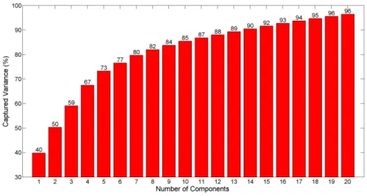
Figure 3.13: Captured variance in the FVA data by PCA vs the number of components. ...39
Figure 3.14: Comparison between PCA and scaled FVA data. A: Biomass data. B: Lactate date. C: Glucose data. D: Ammonia data. E: Alanine Data. F: Essential amino acids data. Number of components: Four (○), five (○), six (○), seven (○). ...40
Figure 3.15: Principal components, loadings, and cont ribution to explain each reaction. 41
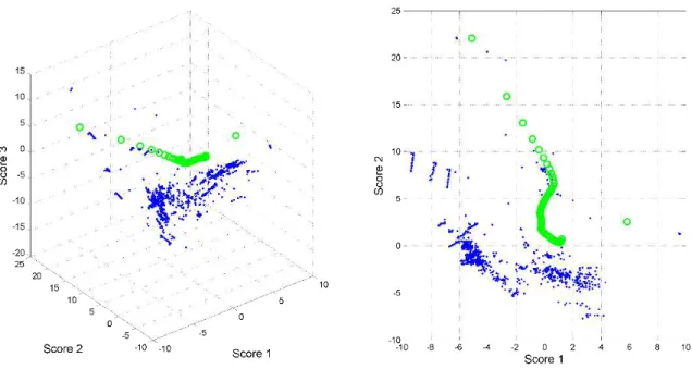
Figure 3.16: Score plot of PCA scores from the FVA data. A: 3D score plot. B: 2D score plot. FVA scores (■), MFA scores (○). ...42
Figure 3.17: Plot of PCA scores from the FVA data and scores for each FBA optimal for each compound deletion simulation. A: 3D score plot. B: 2D score plot. FVA scores (■), MFA scores (○), FBA with no predicted growth rate scores (○), FBA with predicted growth rate scores (○). ...43
xix
List of Tables
Table 2.1: Table with p values used for the creation of the cubic smoothing spline for each
concentration. ... 8
Table 3.1: The determined extracellular fluxes (41 -70h) for the avian cells. ...22
Table 7.1: Table with the corresponding known fluxes applied during MFA. ...55
Table 7.2: Intracellular metabolites included on the metabolic model. ...56
Table 8.1: Concentrations and analytic methods used for each compound measurements. Adapted from Lohr et al in [2]...57
xxi
Acronyms
FBA Flux Balance Analysis. MFA Metabolic Flux Analysis. PCA Principal Component Analysis.
mol unity used in chemistry to express the amount 6.022×10²³ atoms.
h-1 hours.
1
1 Introduction
1.1 The avian cell line AG1.CR.pIX
1.1.1 Background
Since the 18th century vaccine research and development has been a constant focus of scientists, allowing novel therapeutic options. With the first vaccine, developed for smallpox dated from 1796, vaccine production has had since a great impact in human health and it is considered a turning point in human evolution. Nowadays, the problems with vaccine production are the high/varying demands and the production processes itself, which is cost intensive and has a relatively low efficiency. Science is driven by the search for a greater efficiency, which comprises cost and timeline minimizations for industrial process, such as vaccine production. Despite this fact, several viral vaccines, including the human influenza vaccine, are still being produced in primary cell lines such as embryonated eggs or chicken embryo fibroblasts [1]–[4]
.
Few continuous cell lines have been developed and are considered safe for the production of vaccines for humans (e.g. MDCK cells and Vero cells) [1]. However, these cell lines have many limitations, such as the low number of passages possible due to genetic instability and scalability [3]. Further, scale up is limited as the cultivation is done in adherent plates and the cells require calf serum supplement [1], [2]. Calf serum is a potential source of contamination and lot-to-lot changes, which leads to heterogeneous products. The heterogeneity, also caused by primary culture use, impairs the quality of the final product. As such, continuous cell lines that proliferate in chemically defined and simple media have been highly regarded as suitable alternatives.
2 One such potential cell line is a new avian cell line, AG1.CR.pIX, developed from sample tissue of Muscovy duck around 2003 by PROBIOGEN [1], [4]. Duck was chosen because it had been found to have no endogenous avian retrovirus (EAV) or endogenous avian leucosis virus (ELV-E) [4], which is a very important indicator for vaccine safety. Furthermore, duck eggs are available from monitored stocks that are free of pathogen. This new cell line resulted from tissue samples of duck embryo, previously tested for various pathogens. The immortalization was performed with adenovirus type 5 E1 genes as these virus are considered to be ubiquitous and therefore safe for human [2]. The transfected genes were E1A and E1B, originated from adenovirus. The transfected gene products have been shown to promote cell cycle progression and interfere with the p53 transcription factor, which persistent activation had been correlated to apoptosis, therefore allowing immortalization [2]. This immortalization has been shown to be stable after a high number of passage (several years) [3]. Further details can be found in [3], [4].
3
1.1.2 The CR.pIX metabolic model
In this thesis, a metabolic model of central metabolism for the avian cell line CR.pIX, proposed by Lohr et al in [1] was used. A metabolic model is the aggregate of all the reactions assumed or verified to occur in any given cell [7]. A reaction constitutes a sequence of probable and observable steps between a set of input and output of metabolites [7]. The overall cellular reactions result in a conversion of substrates into free energy and a large set of metabolites, including precursor metabolites and building blocks for macromolecular synthesis [7]. This set of metabolites is divided in intracellular metabolites, metabolic product or more complex products such as secondary metabolite [7]. Macromolecular pools usually falls in the category constituents of biomass [7]. In this context, the following formalisms are used:
Substrate as a compound present in the medium, which is taken up and directly incorporated or further metabolized by the cell. The substrate is a broad category, ranging from carbon, nitrogen and various minerals source, essentials for cell function [7]. In our case, the substrates are glucose, pyruvate and amino acids (found in Table 7.1, appendix).
Metabolic product as a compound produced by cell that is excreted to extracellular medium as a result of primary or secondary metabolism [7]. In the present case, the metabolic products are lactate, ammonia, uric acid and carbon dioxide.
Intracellular metabolite as all other class of metabolites that is found inside that cell, including intermediary and building blocks [7]. Example of this is glycolytic, TCA cycle and amino acid catabolism intermediates (see list in Table 7.2, appendix).
Flux, as the reaction rate or speed at which a set of reactants is converted into products.
The cells metabolic network is obtained from the integration of the reactions’ stoichiometries. Stoichiometry is based on the law of mass conservation, where the total mass of reactants is equal to the total mass of products. Typically, the amount of product and reactants are defined in ratios of positive integers, as follows:
Equation 1: A general chemical reaction.
...
...
aA bB
yY zZ
4 As stated before a metabolic model includes a set of reactions, and the stoichiometry of each reactions is very important in modelling. In this case, the metabolic model used comprised 97 reactions and 72 metabolites. The pathways included in the model are TCA cycle, glycolysis, pentose pathway, anaplerosis, amino acid uptake and catabolism, transport reactions, MTHF & uric acid synthesis, lipid synthesis, metabolic product release and biomass production.
In Figure 1.1, the metabolic model of central metabolism for the CR.pIX proposed by Lohr et all in [5], is presented.
5 Detailed reactions included in the metabolic network model are presented in Table 8.2, Annex.
1.2 Objectives
1.2.1 General objectives
The main goal of this thesis is to understand which and how certain compounds that are present in the media impact the biomass growth and the physiological state of the cell. Knowledge about this can support the development of optimal media, in which the biomass growth rate is maximized. It can also help to avoid depletion or inhibition when aiming for very high cell densities, a common process goal, since higher biomass concentrations in principle result into higher virus titer.
1.2.2 Specific objectives
The specific objectives in this thesis included:
1. Validate the model of central metabolism
1.1. Determine the extracellular fluxes and the intracellular fluxes;
1.2. Monte Carlos Sampling to determine all the fluxes standard deviations; 1.3. Determine model consistency, using the standard deviations .
2. Use FBA to determine what the objective of the cell is.
3. Apply FVA to study how certain reaction eliminations (tantamount to eliminations of media compounds) affect the flux distribution obtained by FBA, implicitly elucidating the impact on cell growth and the most important reactions related to growth.
7
2 Methods
2.1 Cell culture and sampling
The experimental data used in this study were obtained by Lohr et al in [1], as a result from a batch experiment in 1 L tank reactor well stirred and aerated. Along the process, triplicate samples were taken for off-line analytic analysis. The medium concentration of various substrates and metabolic product as well a viable cell number were measured. The analytic methods used for each concentration measurement are provided in (Table 9.1, annex). The biomass composition and specific dry weight were also determined experimentally . The detailed experimental and analytic procedures are also described in [5], [1].
2.2 Calculation of the uptake and secretion fluxes
2.2.1 Calculation of the fluxes
A differential approach was used to calculate the flux values [8]. Firstly, cubic smoothing spline functions were formulated for the time profiles of the concentrations based on the experimental data for each concentration Ci, including biomass. The smoothing spline is an interpolation method, where a function that simulates a continuous concentration variation is calculated. The function that is minimized to obtain the smoothing spline f is:
8
Equation 2
2 2 21
w(j)
(j) f
(j)
(1
)
( ) D
( )
n
i j
p
C
t
p
x
f x
dx
Where p is a parameter called smooth factor and belongs to the interval [0,1], and j = 1,…,n are the number of points at which concentration data are available. The variable t represents the time at of each entry j, while w represent the weight of each point Ci,j, the default value for the weight is one. The variable β is the piecewise constant weight function, and in the presented cases has a constant value of one. Finally, the D2f denotes the second derivative of f.
With a smooth factor of one (p=1), a smooth curve which goes through every point in a given data set is calculated, whereas for a smooth factor of zero (p=0), a linear curve fit is calculated.
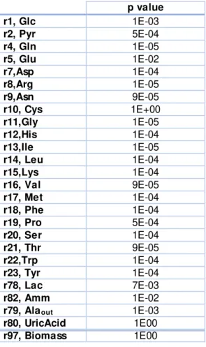
In the following table, Table 2.1, the p values used in this thesis for the creation of the cubic smoothing spline are presented.
Table 2.1: Table with p values used for the creation of the cubic smoothing spline for each
concentration.
p value
r1, Glc 1E-03
r2, Pyr 5E-04
r4, Gln 1E-05
r5, Glu 1E-02
r7,Asp 1E-04
r8,Arg 1E-05
r9,Asn 9E-05
r10, Cys 1E+00
r11,Gly 1E-05
r12,His 1E-04
r13,Ile 1E-05
r14, Leu 1E-04
r15,Lys 1E-04
r16, Val 9E-05
r17, Met 1E-04
r18, Phe 1E-04
r19, Pro 5E-04
r20, Ser 1E-04
r21, Thr 9E-05
r22,Trp 1E-04
r23, Tyr 1E-04
r78, Lac 7E-03
r82, Amm 1E-02
r79, Alaout 1E-03
r80, UricAcid 1E00
9 After the spline of each concentration has been created, the smoothing spline function was differentiated with respect to the time, whereby functions for t he time gradients of substrate uptake and metabolic product releases are obtained. Finally, the homogenous material balances for the reactor were used to calculate the variations of the specific rates (Vi, µmol/gDW/h) along time, where the units of biomass concentration are in dry weight. The glutamine concentration variation was found to be due to chemical decomposition to ammonia and not by cellular uptake as described in [8], [9]. The rate at which this process occurs is a first order reaction with kGln = 0.0032 h-1 obtained from [1]. Based on this, the glutamine and ammonia rates were corrected. The material balance read:
Equation 3 ln
.
.
i i Gln Gln G Amm Amm GlndX
X
dt
dc
v X
dt
dc
v
X
k
Gln
dt
dc
v
X
k
Gln
dt
Where X is the viable cell concentration, t is time and µ is the specific biomass growth rate. The variable vi is the specific rate for each compound (i).
2.2.2 Monte Carlo Sampling for the calculation of the flux standard deviation
10
2.3 Constraint Based Models - Methods for determination and
analysis of the cellular flux distribution
Constraint based methods are yield from the homogenous material balances of the intracellular metabolites:
Equation 4
int
int
.
.
dc
S v
c
dt
assuming a pseudo-steady-state for all intracellular metabolites, meaning that no metabolite accumulation occurs, results in:
Equation 5
int
0
S v
.
.
c
This assumption is usually valid because enzymatic reactions rates take milliseconds, which is very small compared to the biomass growth rate (up to days) [7]. The second term on the right hand side is typically much smaller than the reaction rate values (v), wherefore it is typically neglected. Both assumptions simplify metabolic processes analysis significantly [7]. Detailed description of this assumption can be found in [7]. Furthermore, no kinetics parameters need to be determined for these model applications [10].
Constraint based models can be used for the determination, estimation, prediction and analysis of flux distributions in metabolic networks. These methods allow comprehensive studies of interactions of the pathways in order to identify factors responsible for the control of the overall metabolism [7]. Due to the complexity of biological system, various mathematical methods have been developed in metabolic engineering [11], [12]. These methods are essential for rational metabolic flux modification in order to achieve a certain goal or other application such as medium optimization.
2.3.1 Metabolic Flux Analysis
11 provided that a minimum number of reaction rates are known. MFA does not include kinetic enzymatic parameter of reactions as restrictions. This means incorrect, flux estimations can be observed when compared to in vivo. MFA is based on the pseudo-steady-state assumption, this means that the produced metabolites are consumed at the same rate as they are being produced [7], [10]. This method consists on solving the linear equation problem which consists in the stoichiometric matrix (S) multiplication to the reaction rates vector (v). With pseudo-steady state assumption and neglected growth rate dilution the system reads:
0
S v
.
It is clear that a system of linear equations must be solved in order to obtain each reaction rate (vi). The linear equation system is typically underdetermined as there are more unknown variables than the number of linear equations, i.e. of higher number of reactions than the number of metabolites present in the metabolic model [7]. In another words, in order to solve the linear system a minimum of reaction rates must be determined experimentally. This means that MFA is driven by experimental data, and degree of confidence of the results varies according to the reliability of the latter [7].
With some reaction rates previously determined the linear system can be separated into known (vk,i) and unknown reaction rates (vn,i).
Equation 6 1 # #
,if
,if
0
.
0
.
. v
–
.
. v
un
. . v
. . v
n n k k
n n k k
n n k k
n n k k
n k n n n
S v
S v
S
S v
S
v
S
S
v
S
S is square
S is not square
is Moore
Penrose pseudoinverse
is the known reactions rates
is the
known reac
S
S
tions rat s
v
v
e
Depending on the number of known reaction, the resulting linear system can fall into the following categories, as described in [16].
Determinacy:
12
Determined: rank(Sn) ≥ u a, implying that there are enough linearly independent constraints for computing all rates of vn uniquely.
Redundancy:
Redundant: rank(Sn) < m b, some rows of Sn can be expressed as linear combinations of other rows. In this case, methods for consistency check are applied to verify (and eventually improve) the accuracy of the calculated vn.
Not redundant: rank(Sn ) = m b, system consistent by itself because no dependent rows exist in Sn.
a u = number of unknown rates; b m = number of metabolites.
For any given redundant linear system a redundancy matrix can be obtained by the following equation, as described in [7], [16].
Equation 7 1 #
if
, i
.
.
,
.
.
f
n k n n k k n n k n
R
S
S S
S
R
S is square
S is
S
S S
S
not square
A consistent system fulfils the following conditions, as described in [7], [16],
Equation 8
0
R v
.
kWhile an inconsistent system does not fulfill these conditions. Consistency can be assessed by calculating the ratio between the calculated error of non-balanced metabolites and their estimated variance and comparing the value of this ratio to that of a Chi-square distribution with the same number of degrees of freedom (rank(R)) for a specified confidence value (in this theses .95), for further details see [7]. In case of consistency, detailed procedures to improve the estimated rates (vn) were applied, as well described in more detail in [7].
2.3.2 Flux Balance Analysis
13 is widely used since no kinetic parameter or a minimum number of experimental flux values are required. FBA consists on solving a system linear equations problem.
Given a space of possible biological reactions rates (Upper and Lower boundaries), FBA is used to predict the optimal flux distribution through each pathway given an assumed cellular objective function. This concept is based on the idea that the evolutionary pressure enabled the cells to redirect the metabolic flux according to a certain goal or global objective [21]. It has been shown that the maximization of the cellular growth rate in FBA many times yields flux distributions, which are comparable to measured ones, and it is assumed that this may be due to evolutionary pressure that allowed cells to grow as fast as possible [10], [22]. However, since FBA does not include thermodynamic constraints, e.g. enzymatic parameters, the predicted optimal reactions rate for reactions other than biomass growth rate is usually considerable different from experimental data. In eukaryotic cells it is particularly harder to obtain meaningful physiological steady state with this method, given the more complex cellular behavior and the little information that is used in the predictions [23].
A critical point for the application of this method is the determination of the cell’s biological objective. The objective for which the best fit to the experimental data is obtained using FBA is usually assumed to be the “true” cellular objective.
The following describes how FBA is applied.
Equation 9
1
,
0 reaction
0 reaction
(
)
. v
,
0
.
max
q
i i
v i
l i b
l l
Objective
subject to
i irreversible
i reversi
Z
w
S v
v
v
v
bl
v
v
e
In objective function, the vector w has the same size as reaction vector (v) and it contains positive or negative entries, according to maximization or minimization of the corresponding reaction. S is the stoichiometric matrix.
14
Figure 2.1: Example of FBA applied to a metab olic network, adapted with permission from Macmillan Pub lishers Ltd: Systems-b iology approaches for predicting genomic evolution from [23], copyright
2011.
In Figure 2.1 it is seen that given a set of reactions, a defined space of solution, FBA is then applied to obtain an optimal solution within that space.
2.3.3 Flux Variability Analysis
Flux Variability Analysis is a mathematical optimization methodology used to characterize the solution space of reactions rates in a metabolic model or gene regulatory network , using a set of constraints [17]–[19]. Since the system S*v=0 is typically underdetermined, no unique solution can be obtained by FBA [13], [24]–[26] and FVA can be used to assess the variability of the flux distribution. Other applications include the study of flux distribution under suboptimal conditions, optimization of medium compositions, metabolic flexibility and so on [24].
The following describes the implementation of FVA.
Equation 10
0 reactio
max / mi
n
0 reaction
n
.
0
v v l b l T i lc v
i irreversible
i reversib
S v
v
v
v
v
v
le
15 In metabolic engineering, FVA is essential in the analysis of cellular metabolic flexibility as it allows the determination of the boundaries of each flux for different environmental conditions or mutations [27].
2.3.4 Principal Component Analysis
Principal Component Analysis (PCA) is statistical procedure that uses orthogonal transformation to convert a set of possible correlated data into a set of linearly uncorrelated data [26], [28].
In PCA a matrix of data, X, is decomposed into matrices of loadings W and scores T such that a maximum amount of variance of the data is captured in an underlying latent space for a specified number of latent variables or number of components (p).
Equation 11
is m x n
m x
1
x
components
;
W is
p
T is
p
p is the number of
X
WT
X
The scores describe the patterns of the data in the underlying (orthogonal) latent space and the loadings described the relation between the latent space and the patterns of the data. The PCA loadings are determined in an iterative procedure from the data, X, such that for each latent variable a maximum of variance of the data can be captured.
17
3 Results and discussion
3.1 Cell culture
3.1.1 Exponential biomass growth phase
The overall cell metabolism dynamics have an impact on the biomass growth [7]. As such, the quantification of the biomass concentration is essential for metabolic flux determination and analysis [10].
The experimental data used in this thesis were obtained through a batch experiment in 1 L stirred tank reactor well stirred and aerated. Along the process, triplicate samples were taken for off-line analytic analysis. The biomass composition and specific dry weight were determined as described elsewhere [1]. The detailed experimental and analytic procedures are also described in [1]. In Fig.3.1, the measured viable biomass concentration is presented in relation to the time for the exponential growth phase.
18
Figure 3.1: Biomass exponential growth curve.
It can be seen that the biomass concentration increases, where biomass duplication takes up to two days.
Metabolic Flux Analysis (MFA) is based on a quasi-steady state assumption, meaning that the intracellular metabolite concentrations are almost constant along time [7]. Due to this assumption, the considered time frame of the biomass exponential growth phase for MFA and flux variability analysis (FVA) is from 41-70 hours (R2 is 99.999%). During this phase, it is very likely that the quasi steady state assumption holds [1], [29]. Furthermore, this is the typical growth period before the infection in virus production processes [1], [3].
19
Figure 3.2: Measurements and linear regression model of the b iomass concentration in l ogarithmic scale over time for the exponential growth phase.
3.1.2 Substrates and metabolic products
In order to validate the metabolic model with as much information as possible and to minimize the errors caused by the experimental variations (peaks), data interpolation was performed. The interpolation should on the one side approximate the data well and be within the standard deviation of each measurements, but on the hand be rather smooth without too much low frequency variations. The interpolation is a function that simulates a continuous concentration variation. In this case, the cubic smoothing spline interpolation was performed using the csaps function available in MATLAB®. For each concentration the following functions was defined:
Equation 12
1
... ],
2 1c ... c ], p
2( )
([
n[
n)
F c
cs
aps t
t
t
c
Where ti is time, ci is the concentration and p is the smooth factor, and varies between zero and one.
20
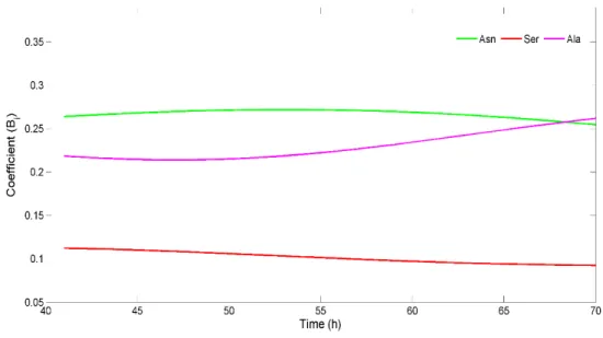
Figure 3.3: Typical variations in sub strate uptake and metab olic product formation for CR.pIX cells cultivation. Black line: interpolation. A: extracellular concentration of glutamine (
■
) and ammonia (♦
). B: extracellular concentration of glucose (▲) and lactate (▼). C: extracellular concentration ofserine (
●
) and glycine (◄).From the analysis of these extracellular concentrations’ variations important conclusions can be drawn. First, the ammonia concentration is very low (Fig. 3.3A) when compared to other cell lines, which is very beneficial as ammonia release inhibits cell growth and has a negative impact in product formation [1]. Secondly, the glutamine uptake is zero and the variation in the media concentration is accounted for by glutamine hydrolyses.
A high glucose consumption can also be observed, in Fig. 3.3B, followed by lactate production and release into the medium. Most likely, almost all of the glucose is converted into lactate even in a well-oxygenated reactor. This is usually termed as aerobic glycolysis, and it is frequently found in cancer cells, although it is an inefficient way to produce ATP [30], [31]. In fact a high aerobic glycolysis is often assumed as a requirement for the increment growth rate, although it is not clear which advantageous it confers to the cancer cells [30], [31]. From a biological point of view the CR.pIX is indeed an abnormal or “cancer” cell as it was immortalized [3]. These metabolic changes can be explained by the fact that transformed cells, like CR.pIX, undergo specific metabolic reprogramming in order to support proliferation [32], [33].
21 both, normal and abnormal cells [33]. Another amino acid with such importance to this cells is serine [32], for which the uptake was observed to be above average. In fact glycine and serine uptakes have been found to be biosynthetically linked [32].
3.2 Metabolic Flux Analysis
Metabolic Flux Analysis (MFA) is a constraint based mathematical method used in metabolic modelling to estimate unknown flux rates distribution for a given metabolic model or network [7]. It is based on the pseudo-steady-state.
The first stage of the work consisted in testing the model previously developed by another group in order access weather it can explain the experimental data. To do this MFA was performed to estimate intracellular flux distribution, followed by a consistency check of the results.
3.2.1 The determined Fluxes
The metabolic model tested in this thesis consists of 97 reactions and 72 metabolites, and the stoichiometric matrix rank is 69. A determined system, in this case, requires a number of at least 28 measured fluxes (97-69). In the present case, these constraints are the uptake rates of substrate and metabolic product formation in the avian cell culture. Other constraints used were the growth rate and the pyruvate carboxylase (r46) which can be set to zero because the enzyme was found to be inactive in [1]. Additional constraints rose from the fact that the same reaction cannot be active both ways, i.e. either uptake or release is observed.
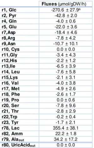
22 In Table 3.1, the determined fluxes mean and standard deviation is presented calculated for the time frame 41-70h.
Table 3.1: The determined extracellular fluxes (41-70h) for the avian cells.
Fluxes (μmol/gDW/h) r1, Glc -270.6 ± 27.9a
r2, Pyr -42.8 ± 2.0
r4, Gln -4.0 ± 0.6
r5, Glu -22.0 ± 3.6
r7,Asp -18.4 ± 4.6
r8,Arg -7.8 ± 4.2
r9,Asn -10.7 ± 10.1
r10, Cys 0.0 ± 0.0
r11,Gly -3.4 ± 4.3
r12,His -2.2 ± 1.2
r13,Ile -6.5 ± 3.9
r14, Leu -7.6 ± 5.8
r15,Lys -2.1 ± 3.1
r16, Val -4.0 ± 3.8
r17, Met -4.9 ± 2.6
r18, Phe -2.6 ± 1.7
r19, Pro 0.0 ± 0.6
r20, Ser -7.8 ± 9.6
r21, Thr -2.8 ± 2.9
r22,Trp -0.2 ± 0.4
r23, Tyr -1.7 ± 2.1
r78, Lac 355.4 ± 38.1
r82, Amm 22.2 ± 1.8
r79, Alaout 34.2 ± 17.2
r80, UricAcidout 0.0 ± 0.0
aStandard deviation calculated from Monte Carlo sampling using experimental measure errors
23
3.2.2 Estimated intracellular fluxes
Using equation (6), previously shown, the substrate uptake and product formation rates and the other mentioned constraints, MFA was performed in order to estimate the intracellular flux distribution.
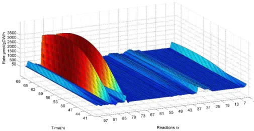
In Figure 3.4, a general overview of both intracellular and extracellular reactions rates variation along the chosen time frame is presented.
Figure 3.4: Metab olic flux distrib ution in CR.pIX.
24 Another aspect of the CR.pIX metabolism is that the uptaken glucose (via r1) seems to be almost all converted into pyruvate (r31) and then to lactate (r32). The amount of pyruvate, which is estimated to enter into the TCA cycle (r33), is much lower than the flux to lactate, implying that the cell in not performing cellular respiration, although it would have sufficient oxygen to perform this task. The amount of ATP generated in this case of lactate production is lower than with oxidative phosphorylation (2 versus 36), but the rate value of the ATP generation is greater [37]. This is in fact, not something new and for cancer cells it is termed aerobic glycolysis or Warburg effect [30], [31], but could apply also to the analyzed cell as discussed above.
On the other hand, levels of the estimated oxygen consumption (r83) and carbon dioxide release rates are also high. The respiration quotient (RQ= CO2/ O2) is 1.06, which is near unity. This is what is expected for a culture supplied with a carbohydrates diet [38], meaning that the flux distribution estimated by MFA might be correct in most of the cases.
3.2.3 Consistency check
25
Figure 3.5: Consistency check results: h-value over time. Test hypostasis X2(0.95, 2) (
̶
).It can be seen that the consistency (h) of the model estimates along time is lower than the test hypothesis (X2(0.95, 2) =5.99), in the considered period. This means the model can explain the flux data [1], [7] and the solution can be considered satisfactory or suitable. On the other hand, the consistency diminishes over time. This could probably mean that although the cells are exponentially growing, the steady state assumption might tend not to hold, when higher cellular concentration is reached [31]. This is most likely due to differential metabolic states, caused by cellular agglomerations or imperfect medium mix. Another explanation for this fact might be that the network used might not fully describe the cells metabolic behavior.
3.2.3.1 Influence of the Error measures in the consistency
26
;
0,1
1
. .
;
1
.
. .
.
new initial i initial
i
new initial i initial
i i initial
h
h
h
n std
n
h
h
n
h
contribution
h
n
n
If we multiply the standard deviation (std) of a specific substrate or metabolic product (i) by a factor (n) and recalculate the system consistency (hnew), then we find a coefficient of contribution of each compound standard deviation (βi) on the overall system consistency. The contribution of each compound is then the coefficient of contribution multiplied by the calculated system consistency.
Since the standard deviation for each compound (stdi) and the overall system h-value (hinitial) changes over time, the coefficient of contribution also changes slightly over time.
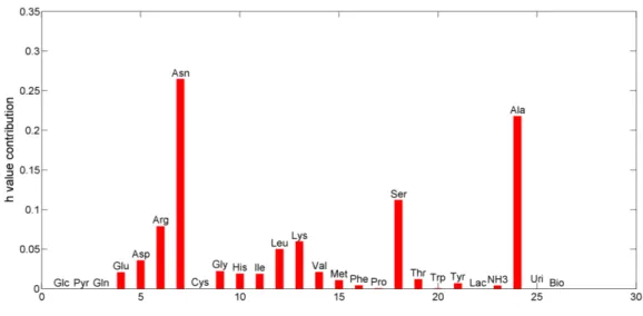
The mean for each estimated contribution coefficient for substrate uptake or metabolic product formation is presented in Figure 3.6.
Figure 3.6: Mean of the coefficient of contrib ution for each of experimentally measured compounds on the model consistency.
27 Surprisingly, there is a differential effect from each substrate standard deviation on the consistency. This suggests that the errors in measurements have different impacts on the overall system consistency. The glucose, pyruvate, biomass and glutamine flux standard deviations have zero impact on the system consistency. On the other hand, asparagine, alanine and serine have a high influence. The metabolic model presented is then highly sensitive to variations in these compounds. These findings suggest that for some compounds a rigorous quantification is uttermost important in order to improve the MFA results for estimated intracellular fluxes. In the following Figure, Fig. 3.7, the coefficient of contribution for compounds that most impact the overall system consistency are presented, over the studied time frame.
Figure 3.7: Coefficient of contrib ution value for compounds with the most impact on the model consistency over time.
This Figure reveals that for the compound for which the measurements errors have the higher influence on the consistency, the coefficients of contribution changes narrowly over time. This highlights their predominance as the main source of the inconsistency.
3.3 Flux Balance Analysis
28 It is also worth mentioning that in more complex systems like eukaryotic cells the objective may be a combination of two or more.
In theory, every cell is considered to have a global objective for a given moment, which governs or directs flux distribution through the metabolic pathways. This goal can change from one environment to another and according to the cell life cycle itself [17]. In the exponential biomass growth phase, this objective usually is the maximization of biomass growth, but this is not always the case [18], [21], [39]. In order to encounter the objective of the analyzed cell, multiple combinations of objective functions, which were taken from literature, were tested (e.g. maximization of ATP production, minimization of reductive power and maximization of lactate production) and the obtained flux distribution compared to the experimental data (data not shown). The objective for which the best fit to the experimental data was obtained, was assumed to describe the cells objective best.
The Linear Programming function (linprog) available in MATLAB® was used to for the FBA calculations. The following parameters where defined:
Upper boundaries (UB)
Lower boundaries (LB)
Objective function (Z)
The problem then reads:
Equation 14: FBA optimization parameters.
2 1
,
reaction
rea
max( )
max
. v ,
0
. v
. v
. v
0
10000
10000
10000
ction
225
v
728
241
v
303
q i i v v o Glc i
n n k k
i i
Z
Objective
subject to
i irreversible
i rev
w
dc
S
S
ersible
S
dt
v
v
29 [21], [40]. Therefore, additional boundary conditions were proposed for the glucose and oxygen flux boundaries. The oxygen and glucose upper boundaries were defined as the sum of the corresponding mean flux value and their standard deviation, calculated from data for the studied phase. The lower boundaries were defined respectively as the sum of the mean flux value minus their corresponding standard deviation. In the studied system, the oxygen boundaries were chosen based on the flux values estimated by the MFA method. Beside the oxygen and carbon source, additional constraints might be needed to avoid futile cycling or unrealistic flux values as shown in [13]. In order to improve the FBA predictability two scenarios were tested, with the same cellular objective and different constraints. The FBA scenarios are described in the following in more detail. In the first, glucose and oxygen boundary conditions were tightened, and in the second scenario, an additional constraint was proposed as a response to the results observed for the first scenario.
3.3.1 The cell objectives
The cellular objective that best describes the experimental data of the CR.pIX cultivation was found to be the minimization of the oxidative phosphorylation occurring in the mitochondria (Z= {Minimization Oxidative Phosphorylation}). This also is in agreement with the observed high lactate production and the lower activity of the TCA cycle found during MFA. This objective was rather unexpected tough the TCA cycle is known to be balanced by the oxidative phosphorylation levels [41] and lower TCA cycle activity means low oxidative phosphorylation.
30
Figure 3.8: Experimental sub strate uptake and metabolic product formation rates plus standard deviations and the rates predicted b y FBA, for the first scenario.
These results reveal that the worst predicted rate is the cysteine rate (355 µmol/gDW/h compared to zero µmol/gDW/h determined experimentally). This over uptake resulted in higher ammonia and lactate estimations. Since the predicted cysteine uptake rate disagrees the most with the observed (see Figure 3.8), in the second tested scenario the cysteine uptake (rcy s=0 µmol/gDW/h) was defined as an additional FBA constraint. It has been reported that the inclusion of uptake rates in the FBA constraints can improve FBA predictions, since it limits the possible solution according to substrate media availability [42], [43].
31
Figure 3.9: Experimental sub strate uptake and metab olic product formation rates, their standard deviations and the rates predicted b y FBA for the second scenario.
In this scenario, the FBA predicts a biomass growth rate of 0.0188 h-1, which is closer to the experimental value of 0.0152 h-1. For most of the tested objective functions (data no shown), the biomass growth rate was well predicted by FBA, whereas the predicted fluxes differed significantly for those fluxes for which experimental data were available. The fluxes that achieve accurate growth rate predictions are not unique but one solution of a large space of solutions [10]. This is one of the main reasons why FBA predictions poorly represent the experimentally measured rates when the objective function is not adequate [10].
In Figure 3.9, it can be seen that most of the predicted flux values are in good agreement with the experimental data, though some fluxes still deviate significantly. Firstly, predicted glutamate and asparagine uptake are both lower than their measured uptake rates. The FBA with this objective compensates these lower fluxes by over uptake of other amino acids like phenylalanine. Phenylalanine catabolism provides the needed glutamine and asparagine and also provides the TCA precursors. FBA with the given objective predicts higher serine flux values than measured. Serine catabolism provides pyruvate that can enter the TCA cycle. It can been seen that estimated ammonia levels are within expected boundaries, which suggest s that amino acids catabolism levels are balanced.
32 The availability of the amino acids present on the media balances the levels of uptake by the cells. In FBA the lack of the predictability of amino acid uptake is because FBA “does not know” how much of what it should assume as the optimal value, if two amino acids give origin to the same needed precursors. Media availability of the substrates dictates the uptake rates when cells are cultivated. In order to improve FBA performance, the environment composition must be an input constraint, as described in [18]. On the other hand, the wide boundaries chosen as constraints can still condition the solutions, even with further constraints.
The lack of predictability of fluxes, i.e. uptake of amino acids, can be accounted for by different reasons, i.e. lack of thermodynamic constraints [10]. A way to improve rate predictions of FBA could be inclusion of a second optimization such as the minimization of the differenc es between predicted and experimentally determined fluxes [44]. It is of interest to use as few as possible constraints to describe the cell’s objective, since in the next step Flux Variability Analysis (FVA) is used to provide ranges of values for each reaction [10]. FBA is a very good method to estimate growth rate, it also very unreliably in predicting other flux values such as metabolic product formation [10]. With few constraints, the solution space is typically wider and the flux variability analysis provides better results [10]. In this scenario, only two out of these 26 predicted flux deviate significantly from the experimental flux values , which is considered to be only a minor defect and so no further constraints were used.
Concluding, a list of causes can be named for the observed deviations: 1) Though the predicted and measured fluxes largely agree the chosen objective function might not completely describe the complex function of the cell. 2) Insufficient large upper and lower bounds or insufficient thermodynamic constraints [45] might in addition contribute to incorrect or infeasible metabolic states. Nevertheless, the selected cellular objective seems to describe the regulation of the levels of oxidative phosphorylation relatively well.
3.4 Flux Variability Analysis
33 into FVA as additional constraints. Various scenarios, where a reaction deletion is simulated, were performed and the solution space for each scenario was calculated using FVA . This task was performed by setting the flux through a given reaction, e.g. amino acid uptake, to zero. Thereupon, FVA is used to obtain the feasible solution space. Important reactions are the most inclined to have lower variability in the flux values and FVA is a promising method for the identification of these reactions [7].
The Linear Programming function (linprog) available in MATLAB® was used to for the FVA calculations. The following parameters where defined:
Upper boundaries (UB)
Lower boundaries (LB)
maxv and minv objectives
The problem then reads,
Equation 15 – The FVA optimization parameters.
1
. 0
reaction
max / min
.
0
.v
min(
)
min
.v ,
.v
0
10000
v v
q
phosporylsation i i
v v i i T
c v
s t
i i
dc
s t
S
dt
v
phosporylsation
w
S
v
rrevers
2reaction
225
728
241
303
10000
0
10000
o G s i lc cyible
i reversib
v
v
v
le
v
3.4.1 Flux variability for FBA results with assumed biological objective
34
Figure 3.10: Rate values predicted b y Flux variab ility analysis for FBA results with assumed b iological ob jective constraint.
Surprisingly only little variations can be seen in Figure 3.10. This means that many predicted rates are uniquely determined by FBA. This phenomena might be due to the constraints (glucose, oxygen and cysteine uptake) used to perform FBA. It was observed that the variabilit y in the fluxes grows when the cysteine constraint is dropped (data not shown). The fluxes that vary most seem to be pyruvate uptake (r2), serine uptake (r20), alanine and glutamate catabolism (r49 and r47) and most of transport reactions (r85, r89, r90-94).
35
3.4.2 Flux variability with different condition environment simulation
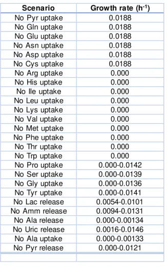
Given the deleted reactions, the biomass growth rate prediction is used to assess the viability of each scenario. In Table 4.2, values of the biomass growth rate predictions are provided for each scenario.
Table 3.2: Growth rate predictions for each tested FVA scenarios.
Scenario Growth rate (h-1)
No Pyr uptake 0.0188
No Gln uptake 0.0188
No Glu uptake 0.0188
No Asn uptake 0.0188
No Asp uptake 0.0188
No Cys uptake 0.0188
No Arg uptake 0.000
No His uptake 0.000
No Ile uptake 0.000
No Leu uptake 0.000
No Lys uptake 0.000
No Val uptake 0.000
No Met uptake 0.000
No Phe uptake 0.000
No Thr uptake 0.000
No Trp uptake 0.000
No Pro uptake 0.000-0.0142 No Ser uptake 0.000-0.0139 No Gly uptake 0.000-0.0136 No Tyr uptake 0.000-0.0141 No Lac release 0.0054-0.0101 No Amm release 0.0094-0.0131 No Ala release 0.000-0.00134 No Uric release 0.0016-0.0146 No Ala uptake 0.000-0.00133 No Pyr release 0.000-0.0121
36 be very beneficial since it diminishes the associated costs with industrial processes . In practice though, this may not be the case. For other amino acids the predicted biomass growth rate is zero when their uptake rates are set to zero. It is very likely that these amino acids are essential.
It can also be seen that when some reactions rates are set to zero, a prediction of partial growth rate is observed. The most interesting result is that when lactate production is set to zero. In this case, the predicted biomass growth rate by the FVA is 33-66% of the experimentally observed growth rate of 0.0188 h-1. If no lactate was produced, most likely cellular respiration would take place. As mentioned above, this is a slower way to produce ATP for biomass growt h [30], which may be the reason why the predicted growth rate is lower. When some amino acids uptake rates are set to zero and a partial biomass growth rate is predicted, this is most likely due to widely known interconversion amino acids [46] .
Overall, these results suggest that the non-essential amino acids are glutamine, glutamate, cysteine, arginine, aspartate and asparagine. These results are in agreement to [34]. Although cysteine is not known to be essential for most eukaryotic cells, it has been found to be essential to avian cells under specific conditions, as reported in [34]. They also suggest that the essential amino acids for CR.pIX are Arginine, Histidine, Isoleucine, Leucine, Lysine, Valine, Methionine, Phenylalanine, Threonine and tryptophan. This also is in agreement to [34]. Finally, partial growth is predicted in FVA results when Proline, Serine, Glycine and Tyrosine uptake rates are set to zero, which is due to the fact that these are considered semi-essential in avian cells [34].
37
Figure 3.11: Rates predicted b y Flux variab ility analysis for all the scenario s where the predicted b iomass growth rate was greater than zero.
It can be seen that most fluxes have a wide range of variation, while others do not. Detailed analysis of this data showed that estimated uptake and catabolism rates of the essential amino acids (such as r8, r12-18, r21-22 and r51-56) have insignificant variation in all scenarios. Another group of estimated reactions rates with insignificant variation is the lipid synthesis (r69-76). Most of TCA cycle reactions also have low variability (such as r35-37 and r41-45). On the other hand, the estimated uptake and catabolism rates for the non-essential amino acids (such as r4-7, r9-11, r20 and r47-50) showed high variations. Another group of reactions with high variability are the transport reactions (r85, r89, r90-94). It can be assumed that the reactions that have the least variability rates through them are likely to be the most important. It has been shown in [27] that the biomass growth rate modulates the cellular metabolic flexibility. Thus, it is very likely that, when the CR.pIX cells are growing, the most important fluxes in order to grow are related to the essential amino acids uptake and catabolism, the lipid synthesis and ATP production via TCA.
3.4.1 The glutamine free medium flux variability
![Figure 1.1: The CR.pIX central metab olic model, adopted from Lohr et al [1] .](https://thumb-eu.123doks.com/thumbv2/123dok_br/16497198.733628/26.893.169.710.324.1034/figure-cr-central-metab-olic-model-adopted-lohr.webp)