An operational system of fire danger rating over Mediterranean Europe

UNIVERSIDADE DE LISBOA

FACULDADE DE CIÊNCIAS

DEPARTAMENTO DE ENGENHARIA GEOGRÁFICA, GEOFÍSICA E ENERGIA

An operational system of fire danger rating over

Mediterranean Europe

[Versão definitiva]

Mestrado em Ciências Geofísicas

Meteorologia

Miguel Neves Mota Pinto

Trabalho de Projeto orientado por:

Carlos da Camara

A

CKNOWLEDGMENTS

This research was performed in the framework of FAPESP/FCT Project Brazilian Fire-Land-Atmosphere System (BrFLAS) (FAPESP/1389/2014 and 2015/01389-4) and of EUMETSAT Satellite Application Facility for Land Surface Analysis (LSA SAF).

Part of methods developed and results obtained are on the basis of the platform supported by The Navigator Company that is currently providing information about weather danger for Portugal for a wide range of users.

R

ESUMO

Os fogos florestais representam um problema sério à escala global para a sociedade moderna. Em particular, a região mediterrânica é afetada regularmente por grandes fogos com impactos negativos aos níveis ecológico, social e económico. Desde 1990 que a Comissão Europeia tem vindo a implementar diversas ações com vista a atenuar o problema dos fogos na Europa, em especial nos países do Sul, sendo de mencionar a implementação de metodologias que visam estimar o perigo de incêndio.

Existem diversos índices para estimar o perigo de incêndio, destacando-se o denominado Fire

Weather Index (FWI) que mostrou ser particularmente útil na região mediterrânica. O FWI foi concebido

originalmente para as florestas Canadianas e, por isso, necessita de ser calibrado para as características da vegetação e condições meteorológicas presentes na região do Mediterrâneo.

Neste estudo procede-se ao desenvolvimento de uma metodologia que permite determinar o perigo de incêndio com base na estimativa de uma probabilidade de excedência de um determinado limiar, previamente definido, de energia diária libertada pelos fogos florestais. Aplica-se o procedimento a uma região da Europa Mediterrânica, delimitada pelos paralelos 35 e 45ºN e pelos meridianos 10ºW e 27.5ºE sobre a qual se define uma malha com a resolução espacial do disco MSG (Meteosat Second Generation), a qual corresponde a cerca de 0.04º em latitude e longitude. Tendo em conta que os dados meteorológicos são referentes às 12h UTC para toda a região, procede-se à sua subdivisão em 5 zonas parcialmente sobrepostas por forma a minimizar as diferenças de fuso horário.

Neste estudo utilizam-se dados meteorológicos, dados de coberto vegetal e dados de incêndios florestais. Os dados meteorológicos provêm das reanálises ERA-Interim produzidos pelo Centro Europeu de Previsão do Tempo a Médio Prazo (ECMWF) e consistem em campos diários, com referência às 12h UTC, de temperatura a 2m, temperatura do ponto de orvalho, componentes zonal e meridional do vento a 10m e precipitação acumulada em 24 horas. Estes dados, com resolução de 0.75º, são reprojetados na malha do MSG aplicando-se uma correção topográfica aos dados de temperatura com base na diferença de topografia entre as malhas do modelo do ECMWF e do MSG e considerando um gradiente vertical de temperatura constante de -0.67ºC/100m. Os dados de coberto vegetal provêm da base de dados GLC2000, que contém 22 tipos de vegetação/uso do solo, os quais se agruparam em três categorias mais gerais – floresta, mato e terrenos agrícolas. Os dados de incêndios florestais são um produto desenvolvido pela Satellite Application Facility for Land Surface Analysis (LSA SAF) a partir de observações dos satélites Metosat, cuja exploração é da responsabilidade da EUMETSAT, a agência europeia para a exploração dos satélites meteorológicos. Para cada ocorrência, recorreu-se a informação acerca da potência radiativa libertada, das coordenadas geográficas, da data e hora e ainda do nível de confiança.

O FWI é calculado diariamente com base nos dados meteorológicos, calculando-se ainda, para cada dia e para cada pixel, as anomalias FWI* relativamente ao respetivo valor médio calculado para o período de 1979 a 2014. A utilização de anomalias FWI*, em vez do FWI, tem a vantagem de atenuar os efeitos devidos à influência da localização geográfica na classificação do perigo de incêndio.

Finalmente, a energia diária libertada pelos eventos de fogo observados em cada pixel e em cada dia é calculada com base nos dados de potência radiativa dos fogos observados remotamente a partir do espaço pelo sensor SEVIRI a bordo dos satélites geostacionários Meteosat. Como a taxa de amostragem dos dados é de 15 minutos, a energia diária é calculada integrando numericamente os valores observados pelo método dos retângulos. De notar que apenas se consideram os fogos cujo nível de confiança atingiu

O procedimento desenvolvido consiste em estimar as denominadas probabilidades estática e diária de excedência de um determinado limiar de energia. Para um dado ponto, a probabilidade estática é estimada pela razão entre o número de ocorrências diárias cuja energia libertada exceda um determinado limiar e o número total de ocorrências no interior de uma célula centrada no ponto. A probabilidade estática é então determinada para vários limiares de excedência, desde 45 a 1800 GJ, e permite definir 𝑛 classes de perigo de incêndio com base nos 𝑛 − 1 quantis para um dado limiar de excedência. Escolhe-se o limiar de excedência de tal forma que a clasEscolhe-se atribuída a um dado pixel apreEscolhe-sente uma fraca dependência no limiar de excedência escolhido. Assim, analisando graficamente a percentagem de pixéis que não mudam de classe quando se tomam limiares consecutivos, escolheu-se o nível de 810 GJ para definir as 𝑛 classes de perigo, número este que, para cada zona, se escolheu empiricamente com base no número de fogos observado durante o período de estudo e no comportamento e qualidade do ajuste dos modelos estatísticos. Obtiveram-se, assim, cinco classes para as zonas A e D, 4 classes para a zona E, 3 classes para a zona C e duas classes para a zona B. Por sua vez, a probabilidade diária de excedência é estimada para cada zona/classe com base numa distribuição de Pareto Generalizada em que o FWI* é uma covariável do parâmetro de escala, a qual integra os fatores meteorológicos.

Combinando a probabilidade estática, que depende apenas da localização geográfica, com a probabilidade diária que tem em conta as condições meteorológicas, obtém-se a uma probabilidade de excedência de determinado nível de energia para um fogo que tenha início em determinado pixel. O racional é que os fogos de pequena dimensão, avaliados através da probabilidade estática, têm uma dependência fraca no estado do tempo, enquanto os grandes fogos dependem fortemente das condições meteorológicas.

Uma das vantagens da metodologia proposta é a de que a probabilidade de excedência permite avaliar o perigo de incêndio com os mesmos critérios para toda a área de estudo, o que torna a probabilidade num bom parâmetro para se harmonizar previsões de perigo de incêndio e estudos de gestão florestal. Com efeito, recorrendo ao histórico de episódios de fogo, mostra-se que as frequências de excedência observadas na área em estudo durante o período 2010-2015 estão de acordo com os valores de probabilidade baseados nos modelos desenvolvidos de probabilidades estática e diária de excedência. A existência de uma (pequena) variabilidade entre os diferentes anos analisados sugere que se proceda a refinamentos em trabalhos futuros mediante a utilização de uma amostra mais vasta a fim de aumentar a robustez do método.

A probabilidade de excedência definida permite uma avaliação física do perigo de incêndio. No entanto é também importante converter esta informação em classes de perigo orientadas para o utilizador comum. Para tal consideram-se break-points de probabilidade de excedência que devem ser calibrados para cada região de interesse a fim de se avaliar de forma ótima as características regionais dos fogos. Analisando as várias ocorrências distribuídas pelas 5 classes de perigo definidas e para vários níveis de energia em forma de tabela verifica-se que, como esperado, os fogos com maior energia libertada concentram-se nas classes de perigo mais elevadas o que se traduz numa forte indicação de que as condições meteorológicas desempenham um papel determinante no desenvolvimento de grandes incêndios florestais. Verifica-se ainda que as probabilidades de excedência de 900 GJ para as regiões consideradas estão de acordo com os break-points de probabilidade de excedência definidos.

Finalmente, em apêndice, faz-se uma breve descrição de uma página web desenvolvida para divulgação diária e em tempo real da previsão do perigo de incêndio e da probabilidade de excedência.

PALAVRAS-CHAVE

Perigo de incêndio, gestão de fogos florestais, distribuição de Pareto generalizada, deteção remota.

A

BSTRACT

A methodology is presented to assess fire danger based on the probability of exceedance of prescribed thresholds of daily released energy. The procedure is developed and tested over Mediterranean Europe, defined by latitude circles of 35 and 45ºN and meridians of 10ºW and 27.5ºE, for the period 2010-2015.

The procedure involves estimating the so-called static and daily probabilities of exceedance. For a given point, the static probability is estimated by the ratio of the number of daily fire occurrences releasing energy above a given threshold to the total number of occurrences inside a cell centred at the point. The daily probability of exceedance which takes into account meteorological factors by means of the Canadian Fire Weather Index (FWI) is estimated based on a Generalized Pareto distribution with FWI as covariate of the scale parameter. The rationale of the procedure is that small fires, assessed by the static probability, have a weak dependence on weather, whereas the larger fires strongly depend on concurrent meteorological conditions.

Probability of exceedance allows evaluating fire danger with the same criteria for all the study area, making it a good parameter to harmonize fire danger forecasts and forest management studies. Probability of exceedance further allows defining a set of 5 classes of fire danger by breaking up levels of probability of exceedance. These levels should be calibrated for each region of interest in order to best evaluate the regional fire characteristics.

It is shown that observed frequencies of exceedance over the study area for the period 2010-2015 match with the estimated values of probability based on the developed models for static and daily probabilities of exceedance. Some (small) variability is however found between different years suggesting that refinements can be made in future works by using a larger sample to further increase the robustness of the method.

KEYWORDS

C

ONTENTS

1 INTRODUCTION ... 1

2 DATA ... 2

 2.1METEOROLOGICAL DATA ... 3

 2.2VEGETATION COVER ... 3

 2.3FIRE RADIATIVE POWER ... 4

3 METHODOLOGY ... 4

 3.1FIRE WEATHER INDEX ... 4

 3.2DAILY ENERGY ... 5

 3.3STATIC PROBABILITY OF EXCEEDANCE ... 5

 3.4STATISTICAL MODELS OF FIRE RADIATIVE POWER ... 6

 3.5DAILY PROBABILITY OF EXCEEDANCE AND FIRE DANGER ... 7

4 RESULTS AND DISCUSSION ... 7

 4.1GENERAL CHARACTERISTICS OF VEGETATION AND FIRES ... 7

 4.2STATIC PROBABILITY OF EXCEEDANCE ... 8

 4.3CLASSES OF FIRE DANGER ... 10

 4.4STATIC MODELS ... 11

 4.5DAILY MODELS ... 13

 4.6DAILY PROBABILITY OF EXCEEDANCE ... 15

 4.7FIRE DANGER ... 17

5 CASE STUDIES ... 19

 5.1CASE STUDY 1–AUGUST 8TH_,2012 ... 19

 5.2CASE STUDY 2–SEPTEMBER 3RD_,2012 ... 20

 5.3CASE STUDY 3–MARCH 28TH_,2012 ... 21

6 CONCLUSIONS ... 23

7 REFERENCES ... 24

APPENDIX I - WEBPAGE ... 26

 DATA ACQUISITION AND STORAGE ... 26

 DATA PROCESSING AND UPLOADING ... 26

L

IST OF

F

IGURES

FIGURE 2.1.THE FIVE OVERLAPPING ZONES (A TO E) THAT COVER THE STUDY REGION OVER MEDITERRANEAN EUROPE... 2

FIGURE 2.2.TOPOGRAPHY OVER THE STUDY AREA. ... 3

FIGURE 2.3.VEGETATION TYPES/LAND USE AS DERIVED FROM THE GLC2000 DATABASE. ... 4

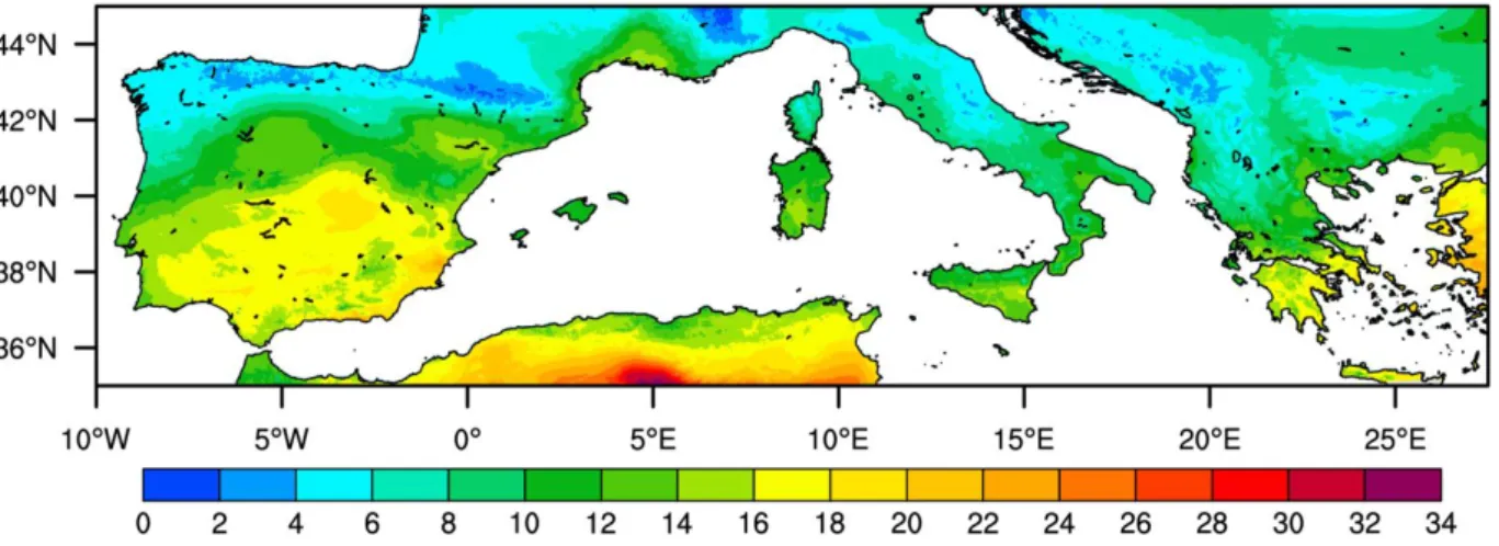
FIGURE 3.1.AVERAGE VALUES OF FWI FOR THE PERIOD 1979-2014. ... 5

FIGURE 4.1.STATIC PROBABILITY OF EXCEEDANCE OF 90GJ. ... 8

FIGURE 4.2.AS IN FIGURE 4.1 BUT FOR THRESHOLD OF 810GJ. ... 8

FIGURE 4.3.SIZE OF CELLS 𝛿 OVER THE STUDY AREA ... 9

FIGURE 4.4.AS IN FIGURE 4.3, BUT FOR TOTAL NUMBER 𝑆 OF FIRE OCCURRENCES WITHIN EACH CELL. ... 9

FIGURE 4.5.PERCENTAGE OF PIXELS BELONGING TO THE SAME CLASS FOR TWO CONSECUTIVE THRESHOLDS OF RELEASED ENERGY FOR EACH ZONA A TO E. ... 10

FIGURE 4.6.CLASSES OF FIRE DANGER FOR ZONES A TO E. ... 11

FIGURE 4.7.QUANTILE-QUANTILE PLOTS FOR FITTED GP DISTRIBUTIONS FOR CLASSES DEFINED AT EACH ZONE A TO E. .... 12

FIGURE 4.8.AS IN FIGURE 4.7 BUT FOR THE CUMULATIVE DISTRIBUTION FUNCTIONS. ... 13

FIGURE 4.9.AS IN FIGURE 4.7 BUT FOR THE DEPENDENCE OF THE SCALE PARAMETER 𝜎 ON 𝐹𝑊𝐼 ∗.THE STRAIGHT DASHED LINES REPRESENT THE CORRESPONDING MAXIMUM LIKELIHOOD GP MODELS WITH A LINEAR DEPENDENCE OF 𝜎 ON 𝐹𝑊𝐼 ∗(𝜎 = 𝑎 × 𝐹𝑊𝐼 ∗ +𝑏). ... 14

FIGURE 4.10.CUMULATIVE DISTRIBUTION FUNCTIONS FOR THREE FIXED VALUES OF 𝐹𝑊𝐼 ∗ OF THE DAILY GP MODELS FOR EXCEEDANCES OF 900GJ FOR ALL CLASSES DEFINED AT EACH ZONE A TO E. ... 15

FIGURE 4.11.ESTIMATED VALUES OF 𝑃(900|0) AND EMPIRICAL VALUES OF PROBABILITY DIRECTLY COMPUTED FROM OBSERVATIONS CONSIDERING SUCCESSIVELY ALL YEARS BUT ONE (TOP PANELS WITHOUT 2010,2011 AND 2012 AND BOTTOM PANELS WITHOUT 2013,2014 AND 2015 RESPECTIVELY FROM LEFT TO RIGHT).COLOURS OF CURVES IDENTIFY THE ZONE. ... 16

FIGURE 5.1.𝑃(900|0) PROBABILITY OF EXCEEDANCE, FIRE DANGER MAP AND OBSERVED FIRES (TOP, CENTRE AND BOTTOM MAPS RESPECTIVELY) FOR AUGUST 8TH,2012. ... 20

FIGURE 5.2.AS FOR FIGURE 5.1 BUT FOR SEPTEMBER 3RD,2012. ... 21

FIGURE 5.3.AS FOR FIGURE 5.1 BUT FOR MARCH 28TH,2012. ... 22

L

IST OF

T

ABLES

TABLE 4.2.SAMPLE SIZE AND RESPECTIVE PERCENTAGE RELATIVE TO THE TOTAL SAMPLE FOR EACH ZONE AND CLASS, FITTED VALUES OF SHAPE AND SCALE PARAMETERS OF GP DISTRIBUTION (WITH 95% CONFIDENCE INTERVALS IN BRACKETS) AND CONFIDENCE LEVEL OF THE ANDERSON-DARLING TEST. ... 12

TABLE 4.3.SHAPE PARAMETER (𝛼), SLOPE 𝑎 AND INTERCEPT 𝑏 OF THE LINEAR MODEL 𝜎 = 𝑎 × 𝐹𝑊𝐼 ∗ +𝑏; AND P-VALUE (%) FOR EACH ZONE AND CLASS. ... 14

TABLE 4.4.BREAK-POINTS OF PROBABILITY OF EXCEEDANCE FOR ZONES A,C AND D AND E... 17

TABLE 4.5.DISTRIBUTION OF FIRES (2010 TO 2015) AMONG THE CLASSES OF FIRE DANGER FOR 5 INTERVALS OF RELEASED ENERGY FOR ALL STUDY AREA. ... 17

TABLE 4.6.AS IN TABLE 4.5 BUT FOR ZONE A. ... 18

TABLE 4.7.AS IN TABLE 4.5 BUT FOR ZONES C AND D. ... 18

1 I

NTRODUCTION

Forest fires represent a serious problem to modern societies and have been identified as the most important threat to forests in Southern Europe (Requardt et al. 2007). The Mediterranean region is regularly affected by large and destructive wildfires, with great negative impacts at social, economic and ecological levels and causing significant human casualties (González Cabán, 2007). About 65 thousand fires occur in the European Union (EU) every year, burning about half a million hectares and leading to estimated annual losses of 2 billion euros (JRC, 2014).

Since 1990 the European Commission has been implementing actions aiming at the organization of an information system about forest fires and at the development and implementation of advanced methodologies to evaluate forest fire danger and estimate burnt areas at the European scale (San-Miguel-Ayanz et al. 2003). A result from these actions, the Fire Danger Forecast module that integrates the European Forest Fire Information System (EFFIS) is presently considered a reference at the European level (San-Miguel-Ayanz et al. 2012).

Multiple indices have been developed with the aim of evaluating fire danger based on information about meteorological conditions. Adopted by EFFIS, the Fire Weather Index (FWI) has shown to be particularly useful to assess fire danger in the Mediterranean region (Viegas et al. 1999; DaCamara et

al. 2014). However FWI was specifically designed for the Canadian forest and therefore has to be

calibrated to the vegetation cover and meteorological conditions of the Mediterranean region.

In this study a methodology is developed to assess fire danger based on the estimation of the probability of exceedance of predefined thresholds of daily released energy by wild fires. The procedure is applied to Mediterranean Europe and is calibrated with data for the period of 2010 to 2015. First, estimates of static probability for each location are obtained by dividing the recorded number of fires exceeding a given threshold and observed within a cell centred on each pixel, by the total number of fires observed within the same cell. Then it is shown that statistical models based on Generalized Pareto (GP) distributions adequately fit to the observed data of released energy and that these models can be improved by integrating the FWI as a covariate of the scale parameter of the GP distributions. These models provide daily estimates of the probability of exceedance of released energy by fires greater than a predefined threshold, and are hereafter referred to as daily models. The rationale is that small fires have a weak dependence on daily weather whereas larger fires strongly depend on meteorological conditions. Therefore, fire danger in a given location and on a given day may be assessed by combining static and daily probabilities of exceedance. Results are finally validated by comparing observed frequencies of exceedance over the study area for the period 2010-2015 with the estimated values of probability based on the developed models for static and daily probabilities of exceedance.

2 D

ATA

The study covers the period 2010-2015 and the area is defined by latitude circles of 35 and 45ºN and meridians of 10ºW and 27.5ºE. The spatial resolution is that of the Meteosat Second Generation (MSG) disk corresponding to about 0.04º over the Mediterranean region. For all geostationary imagers the ground pixel area increases away from the sub-satellite point, in line with the increasing view zenith angle (Roberts and Wooster, 2008). In order to take into account the lag of solar time across Mediterranean Europe and its effects when using meteorological variables at the same coordinated time (12 UTC), the study area was subdivided into 4 overlapping zones labelled from A to D plus an independent zone labelled E covering the northern coast of Africa (Figure 2.1).

2.1 Meteorological data

Meteorological data were obtained from the ERA-Interim reanalysis generated at the European Centre for Medium-Range Weather Forecasts (ECMWF). The ERA-Interim database includes global atmospheric fields for a wide range of meteorological parameters and covers the period from 1 January 1979 up to the present, being continuously updated with a lag of about 3 months. The meteorological parameters provided by the ERA-Interim reanalysis come as the result of a complex process of data assimilation which combines the observed data and the modelled data in a way to provide a continuum, uniform and consistent set of data for a large number of parameters (Dee 2011).

Selected parameters for the study period are 2m and dew point temperatures, 10m zonal and meridional wind components and accumulated precipitation, all parameters but the latter consisting of daily fields at 12h UTC. For precipitation, data consist of 24h accumulated values, from 12h UTC the day before to 12h UTC the current day. Since the spatial resolution of the reanalysis is about 0.75º, data were re-projected onto the MSG grid. In the case of 2m and dew point temperatures, a topographical correction was performed on the data by applying a constant vertical temperature gradient of -0.67ºC/100m to the difference between the height of the ECMWF model and that of the MSG disk. The topography on MSG grid is shown in Figure 2.2. Relative humidity was computed based on values of 2m and dew point temperatures, according to the Magnus expression (Lawrence 2005).

Figure 2.2. Topography over the study area.

2.2 Vegetation cover

Information about vegetation cover/land use was obtained from the GLC2000 database that was adopted by the Satellite Application Facility for Land Surface Analysis (LSA SAF). Vegetation types were re-projected onto the MSG grid leading to 22 types of vegetation/land use. The 22 vegetation types were then merged into 3 main types as follows: vegetation types 1 to 10 – forest, 11 to 15 – shrubland and 16 to 18 – cultivated areas (Figure 2.3).

Figure 2.3. Vegetation types/land use as derived from the GLC2000 database.

2.3 Fire radiative power

Time series of fire radiative power (FRP) covering the period 2010-2015 were obtained from the LSA SAF. The FRP product is derived using data from the Spinning Enhanced Visible and Infrared Imager (SEVIRI) instrument which operates on-board the Meteosat Second Generation (MSG) series of geostationary EO satellites (LSA SAF 2015). Each active fire location in the study area represents the centre of a pixel with an area varying from about 10 to 30 km2_{. The data base includes for each event a}

diversity of parameters that include the geographical coordinates, the date and time, the fire confidence and the fire radiative power expressed in MW. A full description of all products and respective validation is available on the documentation provided at the LSA SAF site (http://landsaf.ipma.pt/).

3 M

ETHODOLOGY

3.1 Fire Weather Index

The Fire Weather Index (FWI) is a fire danger index which is part of the Canadian Forest Fire Weather Index System (CFFWIS, Van Wagner 1974; Stocks et al. 1989).

Daily values of FWI were computed for the study area using the ERA-Interim reanalysis meteorological data, for the period 1979-2014, re-projected onto the MSG grid. For each pixel and day, the anomaly of FWI, hereafter referred to as 𝐹𝑊𝐼∗_{, is defined as the departure from the respective mean}

of FWI for the considered day over the period 1979-2014. Following DaCamara et al. (2014), the anomaly 𝐹𝑊𝐼_𝑝𝑑∗ _{for the pixel 𝑝 of the MSG grid and for the day 𝑑 is hence defined as}

𝐹𝑊𝐼_𝑝𝑑∗ _{= 𝐹𝑊𝐼}

𝑝𝑑− 𝐹𝑊𝐼̅̅̅̅̅̅̅ (3.1) 𝑝

where 𝐹𝑊𝐼_𝑝𝑑 is the FWI value of the 𝑝 pixel and 𝑑 day and 𝐹𝑊𝐼̅̅̅̅̅̅̅ is the average of FWI for that _𝑝 pixel, computed from the daily values observed from 1979 to 2014 (Figure 3.1). Use of 𝐹𝑊𝐼∗ _instead

of FWI aims at mitigating the impact of spatial variability, allowing to define fire danger classes that will depend less on geographical location.

Figure 3.1. Average values of FWI for the period 1979-2014.

3.2 Daily energy

Daily energy released by fire at each pixel was obtained by integrating the radiative power recorded by SEVIRI in that pixel along the day. Since the data are sampled every 15 minutes the daily energy, 𝐸, in GJ, for each pixel 𝑝 and day 𝑑 may be estimated as:

𝐸_𝑝𝑑 = 0.9 × (∑ 𝐹𝑅𝑃_𝑘 96 𝑘=1 ) 𝑝 (3.2)

where 𝑘 indicates the sequence of 15 minute images for each day. In order to reduce false alarms, computation of 𝐸_𝑝𝑑 was restricted to pixels and days where the maximum value of confidence attained during the considered day and pixel was greater than 90%.

3.3 Static probability of exceedance

Considering the period 2010-2015, static probability of exceedance of a given threshold 𝑥 for each pixel 𝑝 was estimated by counting the total number of daily fire occurrences in pixels with the same vegetation type as 𝑝 located inside a cell (centred in the pixel with initial size 𝛿 = 0.7° in latitude and longitude). The size was then successively enlarged by increments of 0.05° until the maximum size of 10° is attained or the total number of events reaches 200. Denoting by 𝑆𝑝(𝛿, 𝑥) the total number of daily

fires inside cell of size 𝛿 centred at 𝑝 and with released energy exceeding 𝑥 , the probability of exceedance 𝑥 is estimated according to the following expression:

𝑃_𝑝(𝑥|0) =𝑆𝑝(𝛿, 𝑥)

𝑆𝑝(𝛿, 0) (3.3)

where 𝑆𝑝(𝛿, 0) is the total number of observed daily fire events. The rationale is that static

probability of exceedance is expected to present smooth spatial variability over pixels of a given vegetation types but steep changes are to be expected among the different vegetation types.

3.4 Statistical models of fire radiative power

The statistical distribution of daily released energy, 𝐸, is modelled using the ‘peaks over threshold’ (POT) approach (Pickands 1975), which is a commonly used tool to quantify fire danger (de Zea Bermudez et al. 2009; Mendes et al. 2010; Sun and Tolver 2012; DaCamara et al. 2014). The POT approach uses the Generalized Pareto (GP) distribution as a model to assign probabilities to the exceedances of 𝐸 over a predefined threshold, i.e. to values 𝑥 = 𝐸 − 𝐸_𝑚𝑖𝑛 (with 𝐸 > 𝐸_𝑚𝑖𝑛) where 𝐸_𝑚𝑖𝑛 is a prescribed minimum value (de Zea Bermudez and Kotz 2010).

The GP probability density function 𝑔 is given by:

𝑔(𝑥|𝛼, 𝜎) = 1 𝜎(1 + 𝛼 𝜎𝑥) −1−1_𝛼 (3.4) where 𝑥 is the exceedance, and 𝛼 and 𝜎 are the shape and scale parameters. The corresponding GP cumulative distribution function is:

𝐺(𝑥|𝛼, 𝜎) = 1 − (1 +𝛼 𝜎𝑥)

−1_𝛼

(3.5) The minimum threshold 𝐸_𝑚𝑖𝑛 is estimated using the excess means graphical approach (Coles 2001) where the chosen value is such that the sample mean of the values exceeding successive thresholds larger than 𝐸_𝑚𝑖𝑛 becomes a linear function when plotted against the respective thresholds.

Once 𝐸_𝑚𝑖𝑛 is determined, the shape (𝛼) and scale (𝜎) parameters are estimated using the maximum likelihood method (Grimshaw 1993). Goodness of fit is assessed by means of the 𝐴2 _{test (Anderson and}

Darling 1952), a nonparametric test that is especially appropriate for models based on long-tailed distributions (Stephens 1986). Confidence levels for 𝐴2 _{are obtained by randomly generating, for each}

model, 5,000 data samples from the respective GP distribution characterised by each maximum likelihood estimated pair (𝛼, 𝜎) from the original dataset.

For each class and zone, POT is applied to the exceedances 𝑥 of all fire pixels that were recorded during the study period (2010 to 2015). Following DaCamara et al. (2014), obtained models, hereafter referred to as static models, may be improved by incorporating daily anomalies, 𝐹𝑊𝐼∗_{, as a covariate}

of the scale parameter in the GP distribution, in particular by assuming a linear dependence of 𝜎 on 𝐹𝑊𝐼∗_:

𝐺(𝑥, 𝐹𝑊𝐼∗_{|𝛼, 𝑎, 𝑏) = 1 − (1 +} 𝛼

𝑎 × 𝐹𝑊𝐼∗_{+ 𝑏}𝑥) −1_𝛼

(3.6) Estimates of shape parameter (𝛼) and of coefficients of the linear relationship 𝜎 = 𝑎 × 𝐹𝑊𝐼∗_{+ 𝑏}

are again obtained using the maximum likelihood method. Performance of the new alternative models, hereafter referred to as daily models, is compared against the respective null models (i.e. the original static models) by using the so-called standard likelihood ratio test (Neyman and Pearson 1933). The test is based on statistic Λ defined as:

Λ = 2(ln 𝐿′_{− ln 𝐿) (3.7)}

where 𝐿 is the maximum likelihood function of the static model and 𝐿′ is the maximum likelihood function of the daily model.

3.5 Daily probability of exceedance and fire danger

Considering two events, A and B, the conditional probability P(A|B) is given by 𝑃(𝐴|𝐵) =𝑃(𝐴 ∩ 𝐵)

𝑃(𝐵) (3.8) where 𝑃(𝐴 ∩ 𝐵) is the joint probability of 𝐴 and 𝐵. Since the total energy released by a fire always increases with fire duration, if 𝐴 > 𝐵 then 𝑃(𝐴 ∩ 𝐵) = 𝑃(𝐴) so that 𝑃(𝐴│𝐵) = 𝑃(𝐴)/𝑃(𝐵). For 𝑥 > 𝐸_𝑚𝑖𝑛 > 0, the conditional probability 𝑃(𝑥|0) is then given by

𝑃(𝑥|0) =𝑃(𝑥) 𝑃(0)= 𝑃(𝑥) 𝑃(𝐸_𝑚𝑖𝑛) 𝑃(𝐸𝑚𝑖𝑛) 𝑃(0) = 𝑃(𝑥|𝐸𝑚𝑖𝑛) × 𝑃(𝐸𝑚𝑖𝑛|0) (3.9) where 𝑃(𝑥|𝐸_𝑚𝑖𝑛) is given by the daily models and 𝑃(𝐸_𝑚𝑖𝑛|0) can be computed by the method described in section 3.3. Based on quantity 𝑃(𝑥|0) classes of fire danger can be derived by considering break-points on the probability values.

4 R

ESULTS AND DISCUSSION

4.1 General Characteristics of Vegetation and Fires

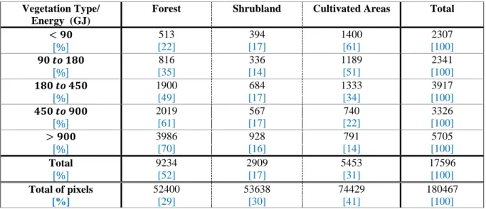
Cultivated areas are the most predominant vegetation type over the study area, accounting for 41%, followed by shrubland with 30% and forest with 29% (Table 4.1, bottom line). Despite being the less abundant type of vegetation, forest accounts for 52% of all observed fires and for 70% of the fires with energy greater than 900 GJ. Shrubland accounts for 17% of the observed fires and cultivated areas for 31% of the fires but only for 14% of the fires greater than 900 GJ. This clearly shows that, as expected, fire dynamics is very distinct among the different vegetation types. Fires with high energy are therefore more common in forest and shrublands than in cultivated areas and forest in particular have the greatest potential for very large fires.

Table 4.1. Distribution of fire energy 𝐸 by vegetation type.

Vegetation Type/ Energy (GJ)

Forest Shrubland Cultivated Areas Total

< 𝟗𝟎 [%] 513 [22] 394 [17] 1400 [61] 2307 [100] 𝟗𝟎 𝒕𝒐 𝟏𝟖𝟎 [%] [35]816 336 [14] 1189 [51] 2341 [100] 𝟏𝟖𝟎 𝒕𝒐 𝟒𝟓𝟎 [%] 1900 [49] 684 [17] 1333 [34] 3917 [100] 𝟒𝟓𝟎 𝒕𝒐 𝟗𝟎𝟎 [%] 2019 [61] 567 [17] 740 [22] 3326 [100] > 𝟗𝟎𝟎 3986 928 791 5705

4.2 Static probability of exceedance

Using the procedure described in section 3.3, values of static probability were computed over the study area for 21 thresholds (namely 45, 90, 180, 270, 360, 450, 540, 630, 720, 810, 900, 990, 1080, 1170, 1260, 1350, 1440, 1530, 1620, 1710 and 1800 GJ).

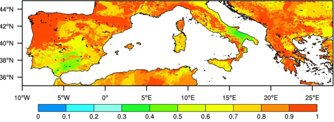
The spatial distributions of values of probability of exceedance for thresholds 90 and 810 GJ, i.e. 𝑃(90|0) and 𝑃(810|0) are shown in Figures 4.1 and 4.2, respectively. The sharp changes of values of probability of exceedance reflect changes in vegetation cover (Figure 2.3). There are wide regions where 𝑃(90|0) is close to 1, indicating that almost all fires observed release more than 90 GJ of energy. On the contrary, for 𝑃(810|0), there are regions where almost no fires exceed the threshold of 810 GJ and therefore fire danger should be lower in those regions.

Figure 4.1. Static probability of exceedance of 90 GJ.

Figure 4.2. As in Figure 4.1 but for threshold of 810 GJ.

The spatial distributions of values of the size 𝛿 of cells (Figure 4.3) and of the total number 𝑆𝑝(𝛿, 0)

of daily fire events within each cell during (Figure 4.4) reflect the characteristics of fires events in Mediterranean Europe. Regions with lower values of 𝛿 have a high density of fire occurrences as opposed to regions of large values of 𝛿 where the density is lower. Regions may be observed, in

It is worth noting that, for example, over Italy, there are regions with high static probability of exceedance (Figures 4.1 and 4.2) that have few occurrences during the study period compared with the surrounding regions (Figure 4.3). This can be explained by looking at the map of vegetation cover (Figure 2.3) where it may be noted that those regions with higher static probability of exceedance correspond to forest while the other regions with lower static probability of exceedance and more fire occurrences mostly correspond to cultivated areas. This visual analysis leads to the conclusion that those cultivated regions have a large amount of fires, but most of them with very small energy released whereas the forest regions have less fires but most of them are large. Looking at the forest regions over north Iberia it may be observed that the number of fires (Figure 4.4) and the static probability of exceedance (Figures 4.1 and 4.2) are both very high. This means that fire danger should be usually higher over these regions.

Figure 4.3. Size of cells 𝛿 over the study area

4.3 Classes of fire danger

As described in the previous section, 𝑛 classes may be defined based on the 𝑛 − 1 quantiles of the static probability of exceedance of a predefined threshold. The number of classes for each zone was empirically chosen based on the number of fires observed during the study period, the goodness of fit of static models and the behaviour of the daily models.

Choice of the optimal threshold was based on the rationale that classes to be defined should be stable in the sense that the class of fire danger attributed to a given pixel should have a very weak dependence on the chosen threshold.

The following procedure was therefore followed:

1. For all threshold considered in section 4.2 – i.e. from 𝑃(45|0) up to 𝑃(1800|0 ), static percentiles of exceedance were computed, classes were defined and pixels were accordingly attributed to a given class.

2. For every two consecutive thresholds, the fraction of pixels that did not change to a different class was computed (Figure 4.5). It is observed that for zones A, D and E curves obtained present a steep increase at lower energy levels but this behaviour is not observed in zones B and C due to the smaller number of classes.

Figure 4.5. Percentage of pixels belonging to the same class for two consecutive thresholds of released energy for each zona A to E.

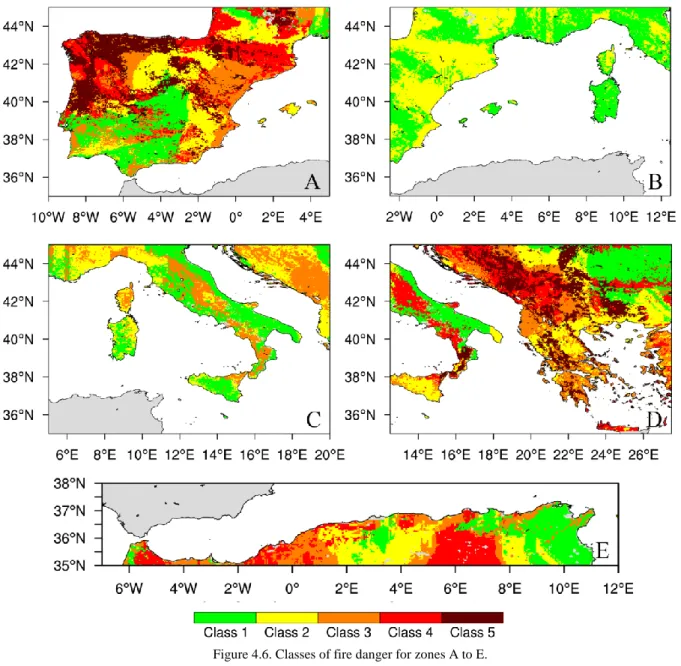
3. Between 720 and 810 GJ the behaviour is similar for all zones and for all remaining changes the curves present a rather stable behaviour, with oscillations of small amplitude for all zones A to E. The optimal threshold was therefore set at 810 GJ, and percentiles of 𝑃(810|0) were therefore chosen to define the static classes for each zone A to E (Figure 4.6).

Figure 4.6. Classes of fire danger for zones A to E.

4.4 Static Models

Choice of threshold 𝐸𝑚𝑖𝑛, for the GP distributions was made by testing successive thresholds, from

0 to 600 GJ with increments of 30 GJ. Values of thresholds were plotted against the respective sample means exceeding each threshold (Coles 2001). For thresholds greater than ~60-90 GJ dependence of exceeding means on thresholds becomes a linear function for each of the 𝑛 classes and 4 zones chosen. The chosen value of 90 GJ presents a confidence level below 93% for all classes and zones, being much lower in most of them, with an average of 34%. This indicates that the null hypothesis that the samples follow GP distribution cannot be rejected at 7% or more significance levels with an average significance level of 66%.

Table 4.2. Sample size and respective percentage relative to the total sample for each zone and class, fitted values of shape and scale parameters of GP distribution (with 95% confidence intervals in brackets) and confidence level of the

Anderson-Darling test.

[ZONE, CLASS] SAMPLE SIZE [%] 𝜶 [95% CI] 𝝈 [95% CI] CL

A1 398 [55%] 0.72 [0.55, 0.89] 152 [126, 183] 17% A2 256 [74%] 0.86 [0.62,1.09] 455 [357, 579] 3% A3 795 [90%] 0.50 [0.39, 0.61] 672 [593, 761] 30% A4 2061 [94%] 0.37 [0.31, 0.43] 913 [849, 982] 81% A5 3606 [96%] 0.40 [0.35, 0.44] 1236 [1170, 1307] 93% B1 261 [82%] 0.89 [0.65, 1.14] 546 [426, 702] 21% B2 265 [98%] 0.71 [0.49, 1.92] 904 [715, 1143] 15% C1 554 [58%] 0.81 [0.65, 0.97] 155 [131, 182] 22% C2 203 [80%] 0.43 [0.21, 0.65] 577 [447, 743] 48% C3 302 [97%] 0.28 [0.14, 0.43] 954 [795, 1146] 3% D1 1210 [65%] 0.33 [0.26, 0.41] 167 [152, 184] 49% D2 612 [71%] 0.61 [0.48, 0.75] 306 [264, 355] 18% D3 516 [87%] 0.56 [0.42, 0.69] 501 [430, 583] 62% D4 330 [92%] 0.36 [0.21, 0.52] 703 [584, 847] 14% D5 412 [98%] 0.20 [0.08, 0.32] 1126 [966, 1311] 3% E1 814 [73%] 0.49 [0.38, 0.59] 274 [243, 310] 5% E2 795 [84%] 0.32 [0.23, 0.41] 480 [428, 538] 7% E3 1258 [86%] 0.33 [0.25, 0.40] 598 [543, 657] 77% E4 1761 [91%] 0.40 [0.33, 0.47] 930 [857, 1009] 78%

The goodness of fit for all classes for each zone can be visually confirmed by analysing the sample quantiles plotted against the GP quantiles (Figure 4.7). Starting at about 7000 GJ energy level it’s observed (Figure 4.7) that the GP quantiles start to overestimate the sample quantiles and this is likely due to the saturation of the sensor that happens for fires of higher power.

The cumulative distribution functions (Figure 4.8) reflect the different behaviours for the different classes. As expected for the lower classes, corresponding to a lower static probability of exceedance of 810 GJ, most fires have lower released energy levels and hence the cumulative distribution function increases to values close to 1 very fast on the low energy levels. The exception is zone B due to having only 2 classes.

It is also observed that, for zones A, D and E where the number of classes is higher, the differences among middle classes are less marked when compared with lowest and highest classes.

Figure 4.8. As in Figure 4.7 but for the cumulative distribution functions.

4.5 Daily Models

Following DaCamara et al. (2014), the role played by FWI on fire activity was evaluated by subdividing the dataset of energy exceedances into 51 groups of fire pixels, corresponding to the values of FWI* starting between the 0 and 50th _{percentiles and moving forward by steps of 1% until reaching}

the 51st _{to 100}th _{percentiles. GP distributions were then adjusted to each group and the estimated values}

of the scale parameter (𝜎) were plotted against the mean FWI* value in the respective range (Figure 4.9). The scale parameter (𝜎) tends to increase with increasing values of FWI* for all zones and classes,

values of the maximum likelihood ratio test are lower than 2.7% (much lower in most cases). The ratio test indicates that the null hypothesis that the daily models have a better fit than the corresponding static ones cannot be rejected at the 2.7% or lower significance level.

Table 4.3. Shape parameter (𝛼), slope 𝑎 and intercept 𝑏 of the linear model 𝜎 = 𝑎 × 𝐹𝑊𝐼∗_{+ 𝑏; and p-value (%) for each}

zone and class.

[ZONE, CLASS] 𝜶 𝒂 𝒃 P-VALUE (%)

A1 0.72 3.5 71.8 0 A2 0.86 13.6 71.4 3 × 10−5 A3 0.50 15.4 301.5 0 A4 0.37 16.4 522.1 0 A5 0.40 27.6 578.0 0 B1 0.89 21.5 67.4 0 B2 0.71 25.1 333.3 0 C1 0.81 5.6 67.4 0 C2 0.43 10.6 329.3 2.7 C3 0.28 24.1 288.5 5 × 10−5 D1 0.33 1.6 140.3 0.04 D2 0.61 7.9 132.7 0 D3 0.56 10.3 257.4 1 × 10−5 D4 0.36 15.1 341.8 9 × 10−4 D5 0.20 20.4 578.6 0.05 E1 0.49 2.5 206.2 0.9 E2 0.32 6.4 300.5 2 × 10−4 E3 0.33 7.6 377.2 0.1 E4 0.40 20.2 303.0 0

It worth noticing that in general for higher classes not only the slope 𝑎 of the linear model is higher (Figure 4.9 and Table 4.3) but the same happens with the value of intercept 𝑏 leading to an even greater difference among classes. It may be noted that a higher value of the slope is an indication of a stronger dependence on 𝐹𝑊𝐼∗_.

The sensitivity of scale parameters to changes in 𝐹𝑊𝐼∗ _{may be put into evidence by plotting the}

cumulative distribution functions for different values of 𝐹𝑊𝐼∗ _{(Figure 4.10). It is worth noting that the}

sensitivity increases from types 1 to 𝑛 provides an indication of the role played by meteorological conditions on the occurrence of large fires.

Figure 4.10. Cumulative distribution functions for three fixed values of 𝐹𝑊𝐼∗ _{of the daily GP models for exceedances of}

900 GJ for all classes defined at each zone A to E.

4.6 Daily probability of exceedance

Values of daily probability of exceedance 𝑃(900|0) are obtained by multiplying values of static probability of exceedance 𝑃(90|0) (as given by the static models) by values of the daily probability of

Results obtained were then verified by comparing values of 𝑃(900|0) with empirical probabilities directly estimated from observations by considering “probability windows” with a width of 0.2 and moving with increments of 0.05 and counting both the total number N of fires occurrences and the number N900 of fire occurrences with energy release above 900 GJ. For each window the corresponding

estimated probabilities (from models) are given by the average of 𝑃(900|0) for all fire occurrences and the empirical probabilities are given by the ratio N900/N.

The robustness of results was assessed by successively comparing 𝑃(900|0) with empirical probabilities for all years but one (Figure 4.11). It may be observed that the differences between estimated and empirical probabilities 𝑃(900|0) is less than 10% for all zones, the exception being zone B where the estimated probability is overestimated. This result is not surprising because zone B is the one with less number of fires and hence the errors are expected to be larger than for the other zones with higher amount of fires during the study period.

The very small variability that is observed in all panels of Figure 4.11 provides a strong indication of the consistency and robustness of the methodology used in the study. It is only in the case corresponding to all years but 2012 (Figure 4.11, top right panel) that a slightly different behaviour is observed, namely for zone B where the overestimation is no longer observed. This difference is explained by noticing that 2012 was the year with higher fire activity during the study period (2010-2015), representing 29% of all the fires that occurred during this period.

Figure 4.11. Estimated values of 𝑃(900|0) and empirical values of probability directly computed from observations considering successively all years but one (top panels without 2010, 2011 and 2012 and bottom panels without 2013, 2014

4.7 Fire Danger

The defined probability of exceedance of energy provides a physically-based assessment of fire danger. However it is also important to convert this information into user-oriented classes of fire danger. Table 4.4 shows the definition of the 5 fire danger classes, respectively labelled Low, Moderate, High, Very High and Extreme, for zones A, C and D, and E. Break-points in probability of exceedance are specifically defined for each one of the 3 regions in order to take into account the different fire behaviours observed. For example, in zone A the probability of exceedance is usually higher than in the remaining zones of the study area, resulting in the occurrence of fires releasing more energy.

Table 4.4. Break-points of probability of exceedance for zones A, C and D and E.

Fire Danger

Class/Zone Zone A Zones C and D Zone E

Low < 0.05 < 0.03 < 0.10

Moderate 0.05 to 0.19 0.03 to 0.14 0.10 to 0.20

High 0.19 to 0.34 0.14 to 0.24 0.20 to 0.30

Very High 0.34 to 0.48 0.24 to 0.35 0.30 to 0.40

Extreme > 0.48 > 0.35 > 0.40

The distributions of fires among the classes of fire danger for 5 intervals of released energy are presented in Tables 4.5 to 4.8 for all study area, zone A, zones C and D, and zone E, respectively. As expected the fires releasing more energy concentrate in the higher danger classes, a strong indication that meteorological conditions play a determinant role in the development of large forest fires.

It is worth noticing that the percentage of fires exceeding 900 GJ for the considered regions (Tables 4.6 to 4.8) is in accordance with the break-points of probability of exceedance as defined in Table 4.4.

Table 4.5. Distribution of fires (2010 to 2015) among the classes of fire danger for 5 intervals of released energy for all study area. Energy (GJ) / Fire Danger Class Low % Moderate % High % Very High % Extreme % Total % < 90 [%] 565 [22] 42 1103 [42] 29 460 [18] 13 320 [12] 7 170 [6] 4 2618 [100] 15 90 to 180 [%] 370 [15] 27 834 [34] 22 498 [21] 14 427 [18] 10 296 [12] 7 2425 [100] 14 180 to 450 [%] 290 [7] 21 994 [25] 27 937 [23] 26 1047 [26] 23 767 [19] 17 4035 [100] 23 450 to 900 [%] 94 [3] 7 478 [15] 13 728 [22] 21 1051 [32] 23 907 [28] 20 3258 [100] 18 > 900 [%] 46 [1] 3 332 [6] 9 920 [17] 26 1662 [32] 37 2300 [44] 52 5260 [100] 30 Total [%] 1365 [8] 100 3741 [21] 100 3543 [20] 100 4507 [26] 100 4440 [25] 100 17596 [100] 100

Table 4.6. As in Table 4.5 but for zone A. Energy (GJ) / Fire Danger Class Low % Moderate % High % Very High % Extreme % Total % < 90 [%] 194 [25] 57 179 [23] 34 121 [16] 11 179 [23] 6 105 [13] 3 778 [100] 10 90 to 180 [%] 88 [12] 26 109 [15] 21 139 [18] 12 248 [33] 8 168 [22] 6 752 [100] 9 180 to 450 [%] 45 [3] 13 128 [8] 24 312 [19] 27 669 [41] 23 467 [29] 16 1621 [100] 21 450 to 900 [%] 4 [0] 1 58 [4] 11 244 [15] 21 698 [43] 23 606 [38] 21 1610 [100] 20 > 900 [%] 10 [0] 3 52 [2] 10 333 [11] 29 1177 [37] 40 1561 [50] 54 3133 [100] 40 Total [%] 341 [4] 100 526 [7] 100 1149 [14] 100 2971 [38] 100 2907 [37] 100 7894 [100] 100

Table 4.7. As in Table 4.5 but for zones C and D.

Energy (GJ) / Fire Danger Class Low % Moderate % High % Very High % Extreme % Total % < 90 [%] 227 [22] 38 612 [60] 33 103 [10] 17 58 [6] 10 16 [2] 3 1016 [100] 24 90 to 180 [%] 179 [20] 30 482 [54] 26 96 [11] 15 84 [9] 14 49 [6] 8 890 [100] 21 180 to 450 [%] 141 [13] 24 462 [43] 25 185 [17] 30 154 [15] 26 128 [12] 22 1070 [100] 25 450 to 900 [%] 42 [7] 7 189 [32] 10 114 [19] 18 133 [22] 22 117 [20] 20 595 [100] 14 > 900 [%] 8 [1] 1 99 [15] 6 123 [18] 20 169 [25] 28 279 [41] 47 678 [100] 16 Total [%] 597 [14] 100 1844 [43] 100 621 [15] 100 598 [14] 100 589 [14] 100 4249 [100] 100

Table 4.8. As in Table 4.5 but for zone E.

Energy (GJ) / Fire Danger Class Low % Moderate % High % Very High % Extreme % Total % < 90 [%] 144 [17] 34 312 [38] 23 236 [29] 13 83 [10] 9 49 [6] 5 824 [100] 15 90 to 180 [%] 103 [13] 24 243 [31] 18 263 [34] 15 95 [12] 10 79 [10] 8 783 [100] 14 180 to 450 [%] 104 [8] 24 404 [30] 29 440 [33] 25 224 [17] 24 172 [13] 18 1344 [100] 25 450 to 900 [%] 48 [5] 11 231 [22] 17 370 [35] 21 220 [21] 23 184 [17] 20 1053 [100] 19 > 900 28 181 464 316 460 1449

5 C

ASE STUDIES

5.1 Case study 1 – August 8

, 2012

Conditions for the occurrence of large forest fires are due to the presence of a very warm air mass over the Mediterranean that reflect on the spread of regions with high probability of exceedance of 900 GJ across the study area (Figure 5.1a).

It is worth noting the distribution of fire danger classes over Italy (Figure 5.1b) where there are regions of very high and extreme fire danger surrounded by large regions of moderate fire danger. This is in agreement with the very distinct probabilities of exceedance of 900 GJ (Figure 5.1a) that reflect the characteristics of vegetation (Figure 2.3); the high probabilities of exceedance of 900 GJ and the very high/extreme fire danger classifications are observed mainly in forest regions whereas the moderate fire danger classification as a result of a probability of exceedance of 900 GJ smaller than 0.1 or 0.2 is observed in cultivated areas. Some of the observed fires exceeded the 900 GJ released energy (Figure 5.1c) and they are mostly located in the Italy regions with higher probability of exceedance of 900 GJ.

A large fire is also observed over Greece (Figure 5.1c) where multiple overlapping dark red dots corresponding to fires exceeding 900 GJ are present. This fire occurred in a region where the fire danger classification was very high/extreme (Figure 5.1b) and the probability of exceedance of 900 GJ was also very high. Similar conclusions can be drawn by analysing the two large fires over Iberia Peninsula (dark red dots in Figure 5.1c).

It is also worth noting the large number of fires occurring in North Africa (Figure 5.1a), some of them in regions of moderate and high fire danger (Figure 5.1b) associated to a not so high probability of exceedance (Figure 5.1a). This behaviour is to be expected over this region since, as shown in Table 4.8, there is a high number of fires occurring in regions of moderate and high fire danger but the fraction of those fires that exceed the 900 GJ released energy level is of course smaller. Nevertheless the number of fires exceeding 900 GJ can be large if the total number of fires is very large, as in the present case.

Figure 5.1. 𝑃(900|0) probability of exceedance, fire danger map and observed fires (top, centre and bottom maps respectively) for August 8th_{, 2012.}

5.2 Case study 2 – September 3

, 2012

During early September 2012 continental Portugal was under the influence of an anticyclone centred over the Bay of Biscay or the British Islands, steering an eastward flow of warm and dry air which resulted in high temperatures and low relative humidity (IPMA 2012).

The probability of exceedance of 900 GJ (Figure 5.2a) reached extreme values exceeding 0.6 in some regions over Portugal and exceeding 0.5 in large areas over Portugal and Spain. The high probability of exceedance of 900 GJ resulted in the extreme fire danger class covering almost all northern Portugal (Figure 5.2b) and a very large amount of fires exceeding the 900 GJ released energy were observed in these region (dark red dots in Figure 5.2c). According to the local press, 15 large wildfires occurred during this day, in very good agreement with the multiple dark red dots (Figure 5.2c), representing fires with more than 900 GJ of released energy.

Some large fires are also observed in Serbia (Figure 5.2c) where fire danger was very high and extreme (Figure 5.2b). It is worth also noticing that, over Italy, the probability of exceedance of 900 GJ was very low on this day resulting in mostly Low and Moderate fire danger classes for the region (Figure 5.2b) and probability of exceedance of 900 GJ smaller than 0.1 (Figure 5.2a).

Figure 5.2. As for Figure 5.1 but for September 3rd_{, 2012.}

5.3 Case study 3 – March 28

, 2012

At the end of March 2012 an unusual amount of fires for this period of the year was observed over northern Portugal and Galicia. This unusual event occurred within a particular meteorological context,

The probability of exceedance of 900 GJ was greater than 0.4 in large areas over northern Portugal and Spain and even greater than 0.5 in a large area over Portugal (Figure 5.3a). This resulted in very high and extreme fire danger classes over the region (Figure 5.3b). Comparing the probability of exceedance of 900 GJ (Figure 5.3a) with the fire danger classification (Figure 5.3b) and the fire occurrences (Figure 5.3c) it may be noticed that most fires take place in regions with very high or extreme fire danger classification where the probability of exceedance of 900 GJ is high and indeed several fires with more than 900 GJ of released energy (dark red dots in Figure 5.3c) were observed.

It is also worth observing that during this day almost all northern Africa that is part of the study area (zone E) presented a low fire danger (Figure 5.3b) with a probability of exceedance of 900 GJ smaller than 10% (Figure 5.3a) and no fires were observed (Figure 5.3c).

6 C

ONCLUSIONS

In this work a methodology was developed to estimate the probability of exceedance of daily energy released by fires over the Mediterranean region. A procedure is also proposed to convert values of probability of exceedance into 5 classes of fire danger. Estimation of probability of exceedance and ranking into classes of fire danger rely on an integrated use of meteorological information provided by ECMWF, vegetation land cover from Global Land Cover 2000 (GLC2000) and fire radiative power as detected by the SEVIRI instrument on-board MSG satellites.

The use of the SEVIRI instrument, with a temporal resolution allowing the detection of fire events every 15 minutes, represents an important advantage in relation to the traditional approaches where the calibration procedures are performed by means of analyses of fire weather history based on ground observations of amount of burned area or on the number of fire occurrences (DaCamara et al. 2014). Use of fire radiative power further provides a solid physical meaning to the approach since energy is a measurable physical property and fire radiative power is directly related to rates of fuel consumption and smoke production (e.g. Wooster et al. 2005). Last but not least, daily probability of exceedance provides a measure of fire danger that is uniform throughout all the study area and may be easily converted into conventional classes of danger.

7 R

EFERENCES

Anderson TW, Darling DA (1952). Asymptotic Theory of Certain "Goodness of Fit" Criteria Based on Stochastic Processes. Annals of Mathematical Statistics 23, 193–212. doi:10.1214/aoms/1177729437.

Coles S (2001). An Introduction to Statistical Modeling of Extreme Values, 208 pp. (Springer-Verlag:London).

DaCamara CC, Calado TJ, Ermida SL, Trigo IF, Amraoui M and Turkman KF (2014). Calibration of the Fire Weather Index over Mediterranean Europe based on fire activity retrieved from MSG satellite imagery. International Journal of Wildland Fire. doi:10.1071/WF13157.

Dee DP, Uppalaa SM, Simmonsa AJ, Berrisforda P, Polia P, Kobayashib S, Andraec U, Balmasedaa MA, Balsamoa G, Bauera P, Bechtolda P, Beljaarsa ACM, van de Bergd L, Bidlota J, Bormanna N, Delsola C, Dragania R, Fuentesa M, Geera AJ, Haimbergere L, Healya SB, Hersbacha H, Holm´ a EV, Isaksena L, Kallberg P, Kohler M, Matricardia M, McNallya AP, Monge-Sanzf BM, Morcrettea J-J, Parkg B-K, Peubeya C, de Rosnaya P, Tavolatoe C, Thepaut JN and Vitarta F (2011). The ERA-Interim reanalysis: configuration and performance of the data assimilation system. Quarterly Journal of the Royal Meteorological Society.

de Zea Bermudez P, Mendes J, Pereira JMC, Turkman KF, Vasconcelos MJP (2009). Spatial and temporal extremes of wildfire sizes in Portugal (1984–2004). International Journal of Wildland

Fire 18, 983-991. doi:10.1071/WF07044.

de Zea Bermudez P, Kotz S (2010). Parameter estimation of the generalized Pareto distribution - Part II. Journal of Statistical Planning and Inference 140, 1374-1388. doi:10.1016/j.jspi. 2008.11.020. González-Cabán A (2007). Wildland Fire Management Policy and Fire Management Economic Efficiency in the USDA Forest Service. Paper presented at the Wildfire 2007-4th International Wildland Fire Conference, 13—17 May 2007, Seville, Spain.

Grimshaw SD (1993). Computing Maximum Likelihood Estimates for the Generalized Pareto

Distribution. Technometrics 35, 185-191. doi:10.2307/1269663.

IPMA (2012). Boletim Climatológico de Março de 2012, (Instituto Português do Mar e da Atmosfera,

http://www.ipma.pt/resources.www/docs/im.publicacoes/edicoes.online/20120405/LLkjsigaQrAr ZyCvbjez/cli_20120301_20120331_pcl_mm_co_pt.pdf

IPMA (2012). Boletim Climatológico de Setembro de 2012, (Instituto Português do Mar e da Atmosfera,

http://www.ipma.pt/resources.www/docs/im.publicacoes/edicoes.online/20121108/bexhlGlAtcjo LwxmGgaO/cli_20120901_20120930_pcl_mm_co_pt.pdf

JRC (2014). Science for Disaster Risk Reduction. EC Joint Research Centre. doi: 10.2788/65084. Lawrence MG (2005). The Relationship between Relative Humidity and the Dewpoint Temperature in

Moist Air, A simple Conversion and Applications. Bulletin of the American Meteorological Society

86, 225–233. doi:10.1175/BAMS-86-2-225.

LSA SAF (2015). Fire Radiative Power Validation Report, Issue II, SAF/LAND/IM/VR_FRP/V_10. Mendes JM, de Zea Bermudez PC, Pereira J, Turkman KF, Vasconcelos MJP (2010). Spatial extremes

of wildfire sizes: bayesian hierarchical models for extremes. Environmental and Ecological

Statistics 17, 1-28. doi:10.1007/s10651-008-0099-3.

Neyman J, Pearson ES (1933). On the Problem of the Most Efficient Tests of Statistical Hypotheses.

Pickands J (1975). Statistical inference using extreme order statistics. The Annals of Statistics 3, 119-131. doi:10.1214/aos/1176343003.

Requardt A, Köhl M, Schuck A, Poker J, Janse G, Mavsar R, Päivinen R (2007).FEASIBILITY STUDY ON MEANS OF COMBATING FOREST DIEBACK IN THE EUROPEAN UNION,ECDGENVCONTRACT, BRUSSEL.http://ec.europa.eu/environment/forests/fpolicies.htm.

Roberts, G.J. and Wooster, M.J (2008). Fire Detection and Fire Characterization Over Africa Using Meteosat SEVIRI, IEEE Trans on Geosci. and Remote Sens., 46, doi: 10.1109/TGRS.2008.915751. San-Miguel-Ayanz J, Barbosa P, Liberta G, Schmuck G, Schulte E, Bucella P (2003). The European

Forest Fire Information System. A European Strategy towards Forest Fire Management. 3rd International Wildland Fire Conference and Exhibition, ITTO, Erickson Air-Crane, FMWG, 3-6 October 2003, Sydney (AUS).

San-Miguel-Ayanz J, Schulte E, Schmuck G, Camia A, Strobl P, Liberta G, Giovando C, Boca R, Sedano F, Kempeneers P, McInerney D, Withmore C, Santos de Oliveira S,, Rodrigues M, Durrant T, Corti P, Oehler F, Vilar L, Amatulli G (2012). Comprehensive Monitoring of Wildfires in Europe: The European Forest Fire Information System (EFFIS). In ‘Approaches to Managing Disaster – Assessing Hazards,Emergencies and Disaster Impacts’. (Ed. J Tiefenbacher) pp. 87– 108. (InTech: Rijeka, Croatia)

Stephens MA (1986). Tests Based on EDF Statistics. In ‘ Goodness-of-Fit Techniques ’ (Eds D'Agostino RB, Stephens MA) pp. 97-193 (Marcel Dekker: New York).

Stocks BJ, Lawson BD, Alexander ME, Van Wagner CE, McAlpine RS, Lynham TJ, Dube DE (1989). The Canadian Forest Fire Danger Rating System: An Overview. Forestry Chronicle 65, 450-457.doi:10.5558/tfc65450-6.

Sun C, Tolver A (2012). Assessing the distribution patterns of wildfire sizes in Mississippi, USA.

International Journal of Wildland Fire 21, 510-520 doi:10.1071/WF10107.

Van Wagner CE (1974). Structure of the Canadian Forest Fire Weather Index. Publication No. 1333,Department of the Environment, Canadian Forestry Service. (Ottawa).

Viegas DX, Bovio G, Ferreira A, Nosenzo A, Sol B (1999). Comparative study of various methods of fire danger evaluation in southern Europe. International Journal of Wildland Fire 9, 235– 246.doi:10.1071/WF00015.

Wooster MJ, Roberts G, Perry GLW, Kaufman YJ (2005). Retrieval of biomass combustion rates and totals from fire radiative power observations: FRP derivation and calibration relationships between biomass consumption and fire radiative energy release. Journal of Geophysical

A

PPENDIX

I

-

W

EBPAGE

Data acquisition and storage

Three-day forecasts from ECMWF available from the LSA SAF are obtained from a webserver through ftp connection using Matlab’s ftp and mget functions. Compressed files are then decompressed using bzip2 command from Cygwin executed through a command line file called from Matlab with

system command. The resulting HDF5 files are then opened in Matlab using the nctoolbox and data are

finally stored in mat format for the European region. These include variables from the Canadian Fire Weather Index System, namely FWI, DSR, FFMC, DC, DMC, BUI and ISI, hereafter called FRM (Fire Risk Mapping) for short.

Information of fire hotspots is obtained on a similar fashion with new data available every 15 minutes. Two mat files are stored for each day, one containing all the observed hotspots with the respective hour and minute of observation and the other with maximum value of energy, maximum fire confidence, starting time, duration of the fire and geographical coordinates for each fire.

Data processing and uploading

The 900 GJ probability of exceedance and the fire danger classes are computed as described in this work. Climatological percentiles 5, 25, 50, 75, 95 are computed using the FRM parameters for the period 1979-2014 using the ERA-Interim reanalysis. For each FRM parameter a class of 1 to 6 is attributed to the value according to the percentile level for the current day. The resulting maps representing the daily FRM percentile classes are plotted in a Mercator projection on Matlab using axesm and geowshow functions. The conversion to a Mercator Projection is required because it is the projection commonly used in web mapping applications. The resulting plots are exported in png format for the FRM, 900 GJ probability of exceedance and Fire Danger. The final step is to set the white background to transparent and then crop the images the most possible in order to decrease their size of storage. This is achieved using Cygwin again and relying on mogrify, a program to process images. As before, the Cygwin commands are called from a command line file executed from matlab using the system command.

Information about hotspots is processed by simply saving a javascript file from matlab where 7 arrays are created to store Latitude, Longitude, Maximum Fire Radiative Power, Maximum Fire Confidence, Hour, Minute and Duration. Processed data are finally uploaded to the webpage using matlab commands

ftp and mput.

Webpage design and content

The webpage was built using javascript, php, html and css relying on the Leaflet javascript library that allows the dynamic display and provides functions to easily add the overlays and the controls to the map.

The map (Figure A1) is projected on the top of the geographical map that allows the usual controls like zooming and moving. The controls at the left allow to change the parameter to be viewed as well as the day of the year (either towards the past to recover available history or for 2 day into the future to obtain forecasts). Fire markers are larger for larger fires and by hovering the mouse over them a small