Behavior and ecology of Caribbean cleaning gobies Elacatinus evelynae in response to reef-condition changes

2017

UNIVERSIDADE DE LISBOA

FACULDADE DE CIÊNCIAS

DEPARTAMENTO DE BIOLOGIA ANIMAL

Behavior and ecology of Caribbean cleaning gobies

Elacatinus evelynae in response to reef-condition changes

Ana Maria Pedrosa Poças

Mestrado em Ecologia Marinha

Dissertação orientada por:

Doutora Marta Soares

Prof. Doutor Carlos Assis

i AGRADECIMENTOS

Obrigada aos meus orientadores, Marta Soares e professor Carlos Assis, por todo o apoio dado, por todos os comentários, incentivos, ajudas e paciência ao longo deste percurso que acabou por ser mais demorado do que o esperado.

Obrigada a todos vocês, Trio Odemira, Cutxis, LC, Cromas, Super Padrinho, F4, Biogado, Sup, que me ajudaram, motivaram, apoiaram ao longo desta tese, por todos os sorrisos, gargalhadas, ralhetes e bons momentos, sem vocês não estaria aqui.

Thank you to all of you, in the Uppsala University for the valuable laboratory lessons, and to all the staff in Carmabi for the help during the field season.

iii

THIS WORK WAS PRESENTED IN THE FOLLOWING SCIENTIFIC MEETING

:

Poças, A.; Santos, T.P.; Messias; J.P.M.; Winberg, S.; Soares, M.C.; (2015). Are coral reef condition and reef fish diversity implicated in cleaning gobies behavior and physiological changes? at 12th congress of the Portuguese Ethological Society, SPE 2015. 9-10th October, Lisbon, Portugal. Book of Abstracts, pag. 22.

v

RESUMO

Os recifes de coral são um dos ecossistemas mais diversos e complexos do planeta. Os corais são formados por organismos simples que vivem em colónias e em relação simbiótica com zooxantelas, que proporcionam nutrientes em troca de abrigo.

O branqueamento dos corais, que se deve à expulsão das zooxantelas, leva à perda das suas cores vibrantes, sendo substituídas por uma coloração esbranquiçada. Este fenómeno pode conduzir à morte dos corais. Estes eventos, na sua maioria motivados por stress térmico, são cada vez mais recorrentes devido às alterações climáticas.

Os parasitas estão presentes e fazem parte da comunidade animal dos recifes, no entanto, evitam o coral vivo, de modo que com a degradação dos recifes e diminuição de coral vivo, os níveis de parasitas podem aumentar. Tal facto leva a um aumento dos níveis de parasitação dos peixes recifais, reduzindo a sua capacidade adaptativa e levando a uma maior vulnerabilidade a infeções.

Um dos mutualismos mais estudado no meio marinho é a relação entre organismos limpadores e peixes maiores que estes, denominados de “clientes”. Nesta, os limpadores inspecionam o corpo dos clientes e removem os ectoparasitas neles presentes. Desta forma, o limpador tem acesso a alimento e os clientes veem reduzida a sua carga parasitária, níveis de stress e um aumento da sua capacidade imunitária. Para dar início a uma limpeza, os clientes podem adotar uma pose imóvel, por vezes quase vertical, de forma a indicar ao limpador que querem ser inspecionados; ou o limpador pode iniciar a mesma sem a demonstração de interesse por parte do cliente. Durante a limpeza podem ainda ser removidas escamas e muco, o que é prejudicial para os clientes, uma vez que estas estruturas os protegem de infeções e têm elevados custos de produção, constituindo portanto uma falha de cooperação. Face a este serviço desonesto, os clientes podem efetuar um movimento de “sacudidela” corporal denominado de jolt. Este estudo teve como objetivo observar se a degradação dos recifes de coral implica mudanças de comportamento, dieta ou níveis de stress numa espécie de caboz limpador, Elacatinus evelynae. Embora esta espécie apresente diferentes níveis de organização social, podendo ser solitários, associarem-se em pares ou em grandes grupos, neste trabalho foram apenas analisados dois tipos de associações: os cabozes solitários e os cabozes que limpam em pares.

Procedeu-se à amostragem de cinco recifes em Curação, uma ilha do sul das Caraíbas. Foram feitos transectos de ponto-intersecção, nos quais foi identificado o tipo de cobertura que aí ocorria (coral vivo, coral morto, coral morto com algas, areia ou outro). Os corais vivos foram posteriormente identificados até ao nível taxonómico mais baixo possível. Foram ainda realizados transectos para analisar a densidade e diversidade da comunidade piscícola. Desta forma, os recifes foram descritos e o seu nível de degradação identificado.

Observaram-se dez estações de limpeza de cabozes limpadores solitários e dez estações de limpeza de cabozes em pares, por recife. O comportamento dos mesmos foi registado considerando: o número de limpezas realizadas, de perseguições pelos cabozes e esperas por parte de clientes que desejavam ser limpos. O tamanho e espécie dos clientes foram também registado. Na ocorrência de uma limpeza, anotou-se a sua duração, quem a iniciava e o número de jolts do cliente. Os indivíduos observados foram capturados e transportados para laboratório onde foram eutanasiados e conservados a - 80ºC. Os seus níveis de cortisol foram posteriormente quantificados.

Adicionalmente foram capturados cinco cabozes solitários e cinco pares de cabozes por recife para serem analisados os seus conteúdos estomacais (parasitas e escamas).

As diferenças entre os recifes foram exploradas com recurso a testes de ANOVA, Kruskal-Wallis, ANOSIM, MDS e SIMPER. Foram utilizados ainda testes de Permanova e GLM’s para verificar a influência do recife nas diferenças encontradas.

vi

Os cinco recifes amostrados foram separados em três categorias: mais degradado, medianamente degradado e menos degradado. Water Factory foi considerado o recife menos degradado (saudável), uma vez que apresentava a maior cobertura (ca. 40%) e diversidade de coral vivo. Carmabi foi considerado o mais degradado uma vez que apresentava a menor cobertura de coral vivo (ca. 3 %) e, apesar de também ter a menor cobertura de coral morto, apresentava a maior cobertura de coral morto com algas (ca. 70 %). Os restantes recifes (Blue Bay Left, Blue Bay Right e Habitat) foram considerados como estando num estado intermédio de degradação, com cerca de 10 % de coral vivo e 45 % de coral morto coberto por algas.

Nos comportamentos de limpeza só se verificaram duas diferenças: os cabozes solitários tiveram maior número de limpezas no recife saudável; nas estações de cabozes em pares, os clientes esperaram mais frequentemente no recife saudável. Todos os outros comportamentos observados, utilizados como medida da qualidade do serviço e motivações dos cabozes e clientes, não variaram entre recifes em nenhum dos contextos sociais.

Entre os parasitas observados no conteúdo estomacal dos cabozes, foram identificados exemplares de duas famílias: Caligidae e Gnathiidae. Não ocorreram diferenças no consumo de caligídeos entre recifes para os cabozes solitários ou em pares. Já no caso dos gnatiídeos, houve um maior consumo destes por parte dos cabozes solitários num dos recifes de condição intermédia de degradação (Habitat). Nos cabozes em pares o maior consumo foi no recife saudável (Water Factory). No consumo de itens não parasíticos, ou seja, indicador de desonestidade do serviço de limpeza, todos os recifes apresentaram valores semelhantes.

Os cabozes solitários apresentaram valores de stress (i.e. cortisol) mais elevado no recife degradado (Carmabi). Tal não se verificou nos cabozes em pares, neste caso, os valores foram semelhantes entre todos os recifes.

O recife onde os cabozes habitam é um fator influenciador da sua dieta e níveis stress. Isto já não se verifica para os comportamentos observados, para os quais o recife não aparenta ser um fator relevante. No geral, não existiram diferenças entre os cabozes solitários e os cabozes em pares que viviam no mesmo recife.

O maior número de limpezas no recife saudável (Water Factory) não se traduziu num maior consumo de parasitas para os cabozes solitários. Desta forma, é proposta a hipótese de que num recife com elevada parasitação, os cabozes possam efetuar menos limpezas, pois têm acesso a um maior número de alimento por limpeza. Enquanto nos recifes com menor parasitação, os limpadores têm de interagir mais vezes para obter a mesma quantidade de alimento.

A inexistência de diferenças entre as estações de limpeza de cabozes em pares nos vários recifes pode dever-se à preferência dos clientes de serem limpos nas estações de cabozes em pares em detrimento das dos cabozes solitários, uma vez que a limpeza a pares aumenta a honestidade do serviço.

O facto de os cabozes solitários apresentarem diferenças de stress entre recifes e os cabozes em pares não, é das primeiras indicações de que os dois grupos reagem de forma diferente à degradação do recife. Adicionalmente, os pares de cabozes apresentam níveis mais elevados de stress do que os solitários, exceto no caso do recife mais degradado. Tal pode dever-se a ser mais vantajoso para os cabozes associarem-se a um parceiro nos recifes degradados.

Apesar destes resultados serem promissores, várias questões ainda permanecem por responder. O maior nível de stress por parte dos cabozes solitários só se verifica no recife mais degradado, não ocorrendo diferenças entre o recife saudável e os medianamente degradados. Permanece assim a questão de qual o limite da degradação do recife para que esta comece a ter impactos nos cabozes. Estudos futuros devem por isso aumentar o número de recifes a amostrar e englobar mais níveis de degradação de forma a tentar identificar melhor qual é a fronteira para esta influência.

Para a maioria das variáveis amostradas não existiram diferenças entre cabozes solitários e em cabozes pares que habitam dentro do mesmo recife.

vii

Neste estudo, não foi possível confirmar se alguma variável caracterizante do recife tinha mais impacto na influência do mesmo nas diferenças de dieta e stress. Foi usado a identidade do recife como um todo, e é por isso relevante que no futuro se explore também esta hipótese.

Este estudo proporciona informação importante para a conservação dos recifes, uma vez que os cabozes limpadores têm um papel ativo nos mesmos, nomeadamente, na manutenção da biodiversidade destes locais.

PALAVRAS-CHAVE: Elacatinus evelynae, degradação de recifes de coral, comportamento de limpeza,

ix

ABSTRACT

Cleaning interactions are among the most studied mutualisms in the marine environment. They not only have a positive impact on both parts (cleaner and client) but also influence the structure of the reef communities by, among other things, increasing biodiversity.

Sharknose gobies, Elacatinus evelyane, and a large number of other cleaning gobies associate with corals, as it is where they maintain their cleaning stations. The increase in coral reef degradation and coral bleaching events affects the parasite proliferation and therefore, goby communities might suffer some kind of impact as well. This study aimed to understand how reef degradation affects these cleaning gobies’ behavior, diet and stress levels.

Five reefs were sampled in Curaçao, South Caribbean. Three different reef health conditions were established - degraded, fair and healthy - by analyzing the fish community (density and diversity), coral diversity and the substratum cover (live and dead coral, sand, and algae). Behavior, diet and stress levels were sampled for both single and paired gobies.

Although some differences in behavior for both single and paired gobies were found between reefs, in healthier reefs single gobies had more cleaning interactions than the degraded one, and paired gobies had more client waits than the fair reefs. However, it seems these were not due to the differences in reef health conditions.

The reef condition was in fact influencing the gobies diet and stress levels. For the diet, single gobies in one of the fair reefs had more intake of parasites than in all the other reefs, and for the paired gobies the higher intake was for the healthier reef. As for stress levels, single gobies were indeed more stressed in the degraded reef than in the fair and healthy ones, but these differences were not observed in paired gobies, as stress levels were similar in all reefs. This indicates that perhaps single and paired gobies react differently to different reef degradation stages, and that it might be more advantageous for gobies in degraded reefs to clean with a partner.

xi

T

C

1.

Introduction ... 1

1.1. Coral Reefs ... 1

1.2. The Caribbean – a region in serious risk? ... 1

1.3. The importance of positive mutualistic interactions to coral reef ecosystems ... 2

1.4. Cleaning gobies ... 3

1.5. Gobies in stress: how are cleaning mutualisms coping? ... 4

1.6. Study objectives ... 5

2.

Materials and methods ... 7

2.1. Study sites and species ... 7

2.2. Coral reef diversity and abundance ... 8

2.3. Reef fish diversity and density ... 8

2.4. Cleaning gobies behavioral observation ... 9

2.5. Cleaning goby diet analysis ... 9

2.6. Tissue Cortisol extraction and determination ... 9

2.7. Statistical analysis ... 10

3.

Results ... 13

3.1. Reef description ... 13

3.2. Cleaning goby behavior ... 17

3.2.1. Single cleaning gobies ... 17

3.2.2. Paired cleaning gobies ... 19

3.3. Diet analysis ... 21

3.4. Cleaning gobies cortisol levels ... 24

3.5. Inside the reef: a comparison between single and paired cleaning gobies ... 26

3.6. A brief summary ... 27

4.

Discussion ... 29

4.1. The health status of the studied reefs ... 29

4.2. Do cleaning gobies have different food consumption between reefs? ... 30

4.3. Do gobies behave differently between reefs? ... 31

4.4. Are gobies from different reefs subjected to different stress levels?... 32

5.

Final remarks ... 35

6.

References ... 37

xiii

L

Figure 2.1- The Island of Curaçao, and the location of the studied reefs (Santos 2016) ... 7 Figure 2.2 – Sharknose cleaning goby, Elacatinus evelynae. ... 8 Figure 3.1 – (a) Mean cover percentage of benthic categories in the sampled reefs. ... 13 Figure 3.2 - Multidimensional scaling plot of benthic community across reefs. Each point corresponds

to a single transect done in Habitat (H), Blue Bay Right (BBR), Blue Bay Left (BBL), Carmabi (C), and Water Factory (WF). Sample size: 10 transects per reef. ... 14

Figure 3.3 – Mean (± SD) number of cleaning stations of: () single goby, (○) paired gobies , () total number of cleaning stations. Sample size for all variables: nBBL= nBBR= nC=nH = nWF=6. ... 15

Figure 3.4 – Mean (± SD) E.evelynae density per m2 _{in the five sampled reefs. Significant differences} are marked with: * Tukey test, p<0.05; ** Tukey test, p<0.01. Sample size: nBBL= nBBR= nC=nH = nWF=6. ... 15

Figure 3.5 – Mean (±SD) fish density (a) and fish diversity (b) in the five sampled reefs. Significant

differences are marked with: : * Tukey test, p<0.05; ** Tukey test, p<0.01. Sample size: nBBL= nBBR= nC=nH = nWF=6. ... 16

Figure 3.6 - Multidimensional scaling plot of the fish community across the reefs. Each point

corresponds to a single transect done in each reef. Sample size: 6 transects per reef. ... 16

Figure 3.7 – Mean frequency of cleaning interactions, cleaner chases and client waits observed in

cleaning stations of single gobies in the five sampled reefs. Significant differences

marked with: * Dunn’s test p<0.05 ... 17

Figure 3.8 – Mean (± SD) average client length (a) and cleaner-client interaction duration (b) at single

goby cleaning stations in the five sampled reefs. Significant differences are marked with: ** Tukey test, p<0.01. Sample size for client size and interaction duration respectively: nWF=7, nBBL=nH=9, nBBR=nC=10; nC=4, nBBL=nH= nWF=6, nBBR=8. ... 18

Figure 3.9 - Likelihood of (a) client posing success, (b) chase by a goby success and proportion of

cleaning events that started by cleaner initiative (c) at single cleaning stations. Box-plots represent median, minimum, maximum, 1st and 3rd quartiles. Mean is marked with “+”. ... 19

xiv

Figure 3.10 - Mean frequency of cleaning interactions, cleaner chases and client waits observed in

pair cleaning stations in the five sampled reefs. Significant differences marked with * and □, Dunn’s test p<0.05 ... 20

Figure 3.11 – (a) Average length of clients visiting paired cleaning stations in the five sampled reefs.

Box-plots represent median, minimum, maximum, 1st and 3rd quartiles. Mean is marked with “+”. ... 20

Figure 3.12 – Likelihood of (a) client posing success, (b) chase by a goby success and proportion of

cleaning events that started by cleaner initiative (c) at paired cleaning stations. Box-plots represent median, minimum, maximum, 1st and 3rd quartiles. Mean is marked with “+”. ... 21

Figure 3.13 – (a) Number of caligids in single cleaning gobies stomachs and percentage of cheating

(c) across five different reefs. Box-plots represent median, minimum, maximum, 1st and 3rd quartiles. Mean is marked with “+”. ... 22

Figure 3.14 –Number of caligids (a) and gnathiids (b)) in paired cleaning gobies stomachs and

percentage of cheating (c) across five different reefs. Box-plots represent median, minimum, maximum, 1st and 3rd quartiles. Mean is marked with “+”. Significant

differences are marked with: ** Dunn’s test, p<0.01. ... 23

Figure 3.15 –Mean (± SD) cortisol levels in single cleaning gobies across the five sampled reefs.

Significant differences marked with: ** Tukey test, p < 0.01. Sample size: nC=5, nBBL=6, nH=nWF=7, nBBR=8 ... 24

Figure 3.16 – Mean (± SD) cortisol levels in paired cleaning gobies across the five sampled reefs.

xv

L

Table 3.1– Total number of client species observed at single and paired cleaning stations ... 17 Table 3.2 - Results of the PERMANOVA analysis conducted to compare the stomach content of

single cleaning gobies between different reefs. Significant p-values (p < 0.05) marked in bold type. ... 22

Table 3.3 - Results of Pairwise PERMANOVA comparisons between reefs for single cleaning gobies

stomach content (p-values). Significant differences (p < 0.05) in bold type. ... 23

Table 3.4 - Results of the PERMANOVA analysis conducted to compare the stomach content of

paired cleaning gobies between different reefs. Significant p-values (p < 0.05) marked in bold type. ... 24

Table 3.5 - Results of Pairwise PERMANOVA comparisons between reefs for paired cleaning gobies

stomach content (p-values). Significant differences (p < 0.05) in bold type. ... 24

Table 3.6 – General linear model test effects for cortisol in single gobies as a dependent variable.

Significant values are marked with bold type (p < 0.05). Model AIC = 215.03. ... 25

Table 3.7 - General linear model test effects for cortisol in individual A of paired gobies as a

dependent variable. Significant values are marked with bold type (p < 0.05). Model AIC = 279.960. ... 26

Table 3.8 – Summary of reef conditions results. ... 27 Table 3.9 – Summary of behavioral, dietary and stress results. ... 28

xvii

A

BBL Blue Bay Left

BBR Blue Bay Right

C Carmabi

H Habitat

WF Water Factory

CS Cleaning stations

1

1. I

1.1. Coral Reefs

Coral reefs are among the most diverse and complex ecosystems worldwide. They support 25% of all marine life, even though they only represent 0.2% of the ocean floor cover (Spalding et al. 2001). Corals are small and simple organisms and can be found in all oceans and at all depths. A large number of species live in large colonies and have the ability to build a shared skeleton. These skeletons can be made of calcium carbonate, making them hermatypic or reef building corals. With only a few millimeters of growth per year, hermatypic corals are frail organisms with a slow growth rate even in ideal conditions, and can be destroyed in only a few hours (e.g. hurricanes) (Spalding et al. 2001). The majority of coral species have a symbiotic relationship with zooxanthellae, providing them shelter while receiving nutrients from their photosynthesis. It is considered that most corals are dependent of these organisms, which in the case of bleaching events is worrisome. Bleaching occurs when the zooxanthellae are expelled or when they lose their chlorophyll. This leads to the loss of corals vibrant colors becoming white or pastel colored (Spalding et al. 2001).

Even though several factors can cause bleaching, the great majority are temperature-related stressors, that are increasing with climate change (Spalding et al. 2001). Coral recovery from bleaching events can occur, although sometimes it is not possible and they perish, turning into rubble and/or becoming covered with sponge and algae, which leads to major reef structure changes (Gardner et al. 2003; Artim and Sikkel 2013). This replacement of live coral for algae is usually known as coral-algae phase shift (Hughes 1994; Bruno et al. 2009) and has an effect on fish assemblages (Done 1992), on fish and invertebrate diversity (Idjadi and Edmunds 2006), and on ectoparasite density (Artim and Sikkel 2013). In addition to this, turf algae directly affects neighboring corals by weakening them, reducing coral fitness and outgrowing them (Birrel et al. 2005; Quan-Young and Espinoza-Avalos 2006; Titlyanov et al. 2007; Barott et al. 2009; Vermeij et al. 2010). It also prevents the settlement of new coral planulae, which leads to a progressive reef degradation that corals cannot overcome (Vermeji and Sandin 2008; Vermeij et al. 2010).

Additionally, reefs are also affected by a plenitude of other conditions such as pollution, coral disease, over-harvesting, storms, nutrient excess, coastal development and sediment pollution (Pandolfi et al. 2003; Bellwood et al. 2004; Hughes et al. 2007; Wilkinson 2008).

Coral degradation is a worldwide crisis, with 19% of the original area of coral reefs already lost (Wilkinson 2008) and with 75% of the world’s reefs threatened (Burke et al. 2011). If no measures are taken this percentage will increase to more than 90% by 2030 and to virtually 100% by 2050 (Burke et al. 2011).

1.2. The Caribbean – a region in serious risk?

The Caribbean represents 7% of the world total reef area and is one of the sites with most reports of reef degradation. It is reported that more than two thirds of Caribbean reefs are threatened, with a considerable part in high and very high risk categories (McClanahan et al. 1999; Spalding et al. 2001; Burke and Maidens 2004; Bruno et al. 2009). In only 30 years, the average hard coral cover on the Caribbean reefs went down from 50% to 10% (Gardner et al. 2003).

Caribbean coral reefs appear to have a lower resilience in relation to other reefs, due to a higher macroalgae productivity (Roff and Mumby 2012). This makes the reefs more prone to suffer algae blooms. In addition, Caribbean functional groups are less diverse and thus if a species disappears, there is a lower capacity to replace its role in the ecosystem (Bellwood et al. 2004). All of this makes Caribbean reefs more frail, vulnerable and their rehabilitation a harder process (Gardner et al. 2003; Bellwood et al. 2004; Roff and Mumby 2012).

2

The chosen study site, the island of Curaçao, is located in the southern Caribbean, north to the coast of Venezuela. It is surrounded by fringing reefs, where more than 70% of all Caribbean species can be found, making the island one of the most diverse areas in the Caribbean (Vermeij 2012). In addition, growing reefs still exist on the island, making this archipelago even more unique. Thus, the coral reefs of Curaçao represent one of the best reef systems left in the Caribbean at present. Yet they also face the same worldwide pressures: coastal development, tourism overuse, pollution and the rise in sea temperature due to climate change (Vermeij 2012). In the past, reef building corals covered approximately 40% of the reefs in Curaçao (Duyl 1985). By 2010 that percentage had decreased by half (Vermeij 2012). If this decline rate continues, even though growing corals still exist, some estimates predict that coral reefs in Curaçao will decline and disappear by 2060 ( Vermeij 2012).

One of the largest threats to coral reefs is the rise in sea temperature, which leads to bleaching events (Wilkinson 2008). In 2010 occurred the worst coral bleaching event ever reported in Curaçao, with 12% of reef building corals being affected (in some locations it went up to 30%). It surpassed the 2005 event that was a record setting for the Tropical Atlantic and Caribbean (Vermeij 2012). This suggests that coral bleaching will start occurring regularly, giving more importance to studies that investigate the impacts that these changes can have (Vermeij 2012).

1.3. The importance of positive mutualistic interactions to coral reef ecosystems

Mutualisms are, by definition, interspecific relationships that result in benefits for all parties involved (Côté 2000). Positive mutualistic interactions are considered to be of key importance for reef fish communities as these make the environment, directly or indirectly, more favorable for associated species, which in turn will facilitate the establishment of other species (Grutter and Irving 2007). At larger regional scales, positive interactions enhance diversity via an increase in habitat diversity (Stachowicz 2001). At a more individual scale, these interactions seem to contribute to an increase of body condition and decreased baseline and acute stress levels.

Cleaning mutualisms can take two forms: an incidental cleaning, which does not require any adaptation on either of the participants, or a cleaning that involves specific behavior and morphology (Côté 2000). An example of the first case occurs between herbivore fishes and sea turtles. In this association the fish eat algae lodged on the body surface of the turtle, just as if they would from the substratum (Losey et al. 1994). The second case involves specialized organisms, known as cleaners, that receive the visit of other often larger organisms (known as clients), to inspect their body in search for ectoparasites, mucus and dead or diseased tissues (Feder 1966; Côté 2000).

During mutualistic cleaning interactions, the cleaners feed on ectoparasites, such as gnathiids and caligid copepods (Arnal and Côté 2000). If not removed, these can lead to host disease, behavior and immunological changes, host fitness reduction, and can even impact host population dynamics (Arnal et al. 2000; Barber et al. 2000; Buchmann and Lindenstrøm 2002; Finley and Forrester 2003; Hudson et al. 2006). Through this, the cleaner gets access to a preferred meal and the clients get their parasite load reduced, preventing or reducing the effects referred above which have a major impact in fish health (Grutter 1999; Arnal and Côté 2000; Arnal et al. 2000; Bshary et al. 2007).

These cleaning interactions promote local reef fish diversity and density, and impacts the structure of reef fish communities (Bshary 2003; Grutter et al. 2003; Bshary et al. 2007).

The sequence of a cleaning interaction may start either with the client posing for the cleaner or with the cleaner first approaching the client (Côté 2000; Soares et al. 2007). Client poses are usually very conspicuous, since clients adopt an immobile posture. All fins are erect and the body almost vertical, remaining motionless throughout all the interaction (Côté et al. 1998). Species have specific poses, although some show variability in their posing behavior (Côté et al. 1998). Cleaners then start inspecting the client’s body surface, inside the buccopharyngeal cavity and the gills chamber, removing ectoparasites, dead or infected tissue and debris (Grutter and Hendrikz 1999; Grutter 2002).

3

Cleaners can remove more than ectoparasites. Sometimes they also remove healthy tissue, mucus and/or scales (Feder 1966; White et al. 2007; Soares et al. 2008a; Campos and Sá-Oliveira 2011). Such behavior is labelled as “cheating”, since mucus protects fish against infections, and due to a high protein content, it is expensive to produce not being beneficial for the client (Ebran et al. 1999; Arnal et al. 2001). Clients keep track of cleaners’ behavior, if the latter provides an honest (remove parasites) or a dishonest (cheat) service. From the client’s perspective, getting immediately inspected and receiving a good service are factors that can evaluate the quality of a cleaning interaction (Bshary and Noë 2003). Cleaners cheating behavior may be measured by jolt count, which are whole-body shudders that are apparently painful reactions to a cleaner fish bite and have been associated to dishonest bites by cleaners (Soares et al. 2008a).

Nevertheless, clients benefit from interacting with cleaners, as it reduces parasite loads, decreases stress levels and the need to have a high immune function. Lower loads and exposure to parasites lead to a reduction in the energy allocated to the immune system, that can be used for other processes such as growing (Bshary et al. 2007; Ros et al. 2011a). Stress reduction may even be a key motivation for clients to seek cleaners (Ros et al. 2011b). Another interesting effect arises from the basic access to physical contact, which also contributes to the reduction of baseline stress levels in clients (Soares et al. 2011).

1.4. Cleaning gobies

Cleaning gobies (Elacatinus spp.) are the most ubiquitous cleaners in the Caribbean region (Soares et al. 2008a). This study focused on sharknose gobies, Elacatinus evelynae (Böhlke and Robins, 1968), which are relatively small (1.2-3.5 cm total length) and have a prominent lateral stripe (blue and yellow) extending from the snout to the tail (Soares et al. 2009).

Although best known for their cleaning behaviors they are sometimes described as facultative cleaners by some authors, due to their alternative habitat related strategies, which may vary between coral heads or basket sponges (Côté 2000; White et al. 2007). When found on coral heads they are cleaners and that is where they maintain their territories (known as cleaning stations) (White et al. 2007). If found on basket sponges, they feed mainly on nonparasitic copepods and spend little time cleaning (White et al. 2007). In this study, only cleaners found on coral heads were considered.

Sharknose gobies can be found alone, in pairs or in groups in their territories and their behavior is known to vary in accordance to their social status (Soares et al. 2008a, 2009).

As in other cleaner species, both scales and mucus have been found in E. evelynae stomach, demonstrating the practice of a dishonest service. However, contrarily to Labroides dimidiatus, the Bluestreak cleaner wrasse, one of the most abundant and well known cleaner in the Pacific, gobies appear to prefer eating ectoparasites (Soares et al. 2010). So it is suggested that gobies start their cleaning interaction just searching for this food item but once it is reduced they start ingesting mucus and scales (Soares et al. 2010).

In order to control dishonest cleaners, clients may either change the cleaning station they visit or respond aggressively by chasing the cleaner (Soares et al. 2008c). On the other hand, some cleaners also manipulate clients into staying after cheating occurs, by providing tactile stimulation with their pelvic fins to the clients’ dorsal region (Soares et al. 2008c). Cleaning gobies however do not have either (Soares et al. 2008c). They do not perform tactile stimulation because they are ultimately honest. This leads to a minimum amount of conflict and to an overall similar quality of service, therefore clients do not need to punish them. Moreover, in the cleaning goby system, clients’ jolts act as a reliable signal that the parasite load is low and that it is time to stop the interaction (Soares et al. 2008c, 2010).

4

1.5. Gobies in stress: how are cleaning mutualisms coping?

Stress can be described as “the nonspecific response of the body to any demand made upon it” (Selye 1973, p. 692). It can also be described as a state of threatened homeostasis by a real or perceived stressor that is re-established by a complex suite of adaptive responses (Chrousos 1998; Barton 2002).

Stressors can vary from predation risk and other antagonistic fish interactions to environmental variables. The degree of reaction to a stressor is variable between species. Some have a high reaction and others an almost unnoticeable one (Iwama 1998; Barton 2002; Soares et al. 2012). However if the stressor is prolonged and severe, it can have an impact on fish health and well-being, from a molecular level to its social organization (Barton and Iwama 1991; Barton 2002).

Fish response to stressors is divided in primary, secondary and tertiary responses (Iwama 1998; Barton 2002). The first include endocrine changes such as the release of catecholamines and corticosteroids (Wendelaar Bonga 1997; Reid et al. 1998; Barton 2002). The second involves metabolic, cellular, hematological and immune function changes and osmoregulatory disturbance (Iwama 1998; Barton 2002). And tertiary responses are related to changes in whole-animal performance and modified behavioral patterns (Iwama 1998; Barton 2002).

Corticosteroids are able to cross blood-brain barrier and access the receptors in the brain. This adds to their importance in stress responses, because, in order to affect behavior, the mediation of stress also has to affect the brain (Nelson 2005; Soares et al. 2012).

Cortisol is the main corticosteroid in teleosts and, contrarily to the catecholamines that are immediately released after a fish is exposed to a stressor, cortisol release is delayed and its effects are more prolonged (Gamperl et al. 1994; Barton 2002; Martinez-Porchas et al. 2009). This allows to sample and measure fish baseline levels of cortisol, and therefore it is commonly used as an indicator of stress in fish (Barton and Iwama 1991; Wendelaar Bonga 1997).

Various studies investigated the relation between the access to cleaning interactions and the clients’ stress levels (Bshary et al. 2007; Ros et al. 2011a). However, few attempted to comprehend cleaners’ stress levels, their variations, and which variables can sway such levels.

Munday (2004) proposed that habitat specialists would be the first species to be lost from coral reefs if degradation occurs. The fact that some cleaning gobies are coral dwellers could mean they are more predisposed to be affected by the degradation in coral reefs. Thus, considering the real pressures of organisms inhabiting coral reefs, particularly those considered to have a key relevance to the community, it is important to know how these are responding to ecosystem shifts, the lowering of fish diversity and changes in food (parasite) availability.

5

1.6. Study objectives

The importance of cleaners, their behavioral abilities and their scope of influence to the remaining fish communities is clearly linked to a necessity to find out more about the underlying mechanisms of these elaborate interactions and how exposed these may be to the present dramatic changes suffered by reef ecosystems. Thus, cleaners are under a significant amount of pressure. Also, the relevant changes in their fish clientele and parasite levels may also translate into cleaning goby physiology changes. Thus, taking this into consideration, this study aims to understand if gobies living in different reefs exhibit:

(1) different behaviors;

(2) different diet and food consumption; (3) different stress levels;

7

2. M

2.1. Study sites and species

This study took place in the southwestern coast of Curaçao, Netherlands Antilles, between June and August 2014. Five reef sites (Figure 2.1), Habitat, Blue Bay Right, Blue Bay Left, Carmabi and Water Factory, were chosen based on visual differences in reef health status and the report ‘The current state of Curaçao's Coral Reefs’ by Mark Vermeij (2012), with the attempt to maximize the differences in fish abundance, diversity and benthic characteristics amongst reefs.

8

The reefs sampled were located on the south west side of the island, which is characterized for having a gradually sloping terrace in front, dropping-off at 7 m to 12 m with a slope that varies from 45° to vertical (Bak 1975). Coral cover and diversity are at the highest near the drop-off, reaching 70% (Vermeij 2012). The studied reefs were distributed along a 21 km stretch of coastline, with distances between reefs that ranged between 300 m to 12 500 m.

The target species in this study was the sharknose cleaning goby, Elacatinus evelynae (Figure 2.2). It is the main cleaning species in the Caribbean, with a high abundance and is easily identifiable (White et al. 2007; Soares et al. 2008c, 2012).

Figure 2.2 – Sharknose cleaning goby, Elacatinus evelynae.

2.2. Coral reef diversity and abundance

Point intersect transects were used to access the quantity and diversity of corals in all the selected five reefs. Ten 10 m long transects were carried out per reef by one diver. In order to categorize the dominant substrate (dead coral, dead coral with algae, live coral, sand and other) annotations were taken every 10 cm, totaling 101 per transect. All living corals were photographed for posterior identification; they were identified to the lowest taxonomical level possible.

2.3. Reef fish diversity and density

In order to analyze reef fish diversity and density, six transects were performed in each reef. Each transect had a total length of 50 m, a width of 4 m and was conducted by two divers. The transect was marked longitudinally with a measuring tape placed in the center of the 4 m width. An assessment dive was performed in which all species observed were photographed and/or described in a plastic board so they could be later identified and a species list compiled. This list was divided in two, so each diver was responsible to count the individuals of a different set of species. The 50 m distance was swam twice.

9

The first time, the species on the list were noted and the number of individuals per species was counted. The second time around, all the cleaning stations and E.evelynae were counted, in this case each diver would get one side of the sampled area (right or left side of the measuring tape). If new species to the list were observed along a transect, a photo or description was taken to allow a posterior identification and addition to the list.

2.4. Cleaning gobies behavioral observation

For each reef a total of 20 cleaning stations were observed, 10 occupied by one adult cleaning goby (single) and 10 operated by two adult cleaning gobies (a pair). The observations were done by three different divers. In order to reduce the error between different observers, preliminary observations were done to ensure that the criteria utilized by all divers was standardized.

The cleaning stations (and thus the cleaners) were chosen haphazardly, between depths of 1 m and 15 m. Each cleaning station was observed once for a period of 20 min, between 10 am and 4 pm, which coincided with the period of cleaning activity in this species (Johnson and Ruben 1988). Observations were made from a distance of 2-3 m. A total of 2000 min of observations were logged by the divers during this study.

All cleaner fish were observed per cleaning station (one or two in the case of a pair). During each observation the species and size (total length estimated to the nearest cm) of each visiting client was registered and, three types of behavior were recorded: waiting to be inspected (when a client is willing to be cleaned and waits to be attended, but it is not), cleaning interactions (when a client is inspected) and cleaner chases (whenever a cleaner pursues a client, trying to start a cleaning interaction, but does not) (Soares et al. 2008a, 2009). Whenever an interaction occurred, its duration was registered as well as which party initiated each interaction: whether the client posed before receiving an inspection (client-initiated) or if the cleaner began the inspection prior to client posing behavior (cleaner-(client-initiated). Finally, the number of jolts performed by the client and if the interaction was terminated with a jolt were also recorded (Soares et al. 2008a, 2009).

2.5. Cleaning goby diet analysis

On each of the focused reefs, 5 singles and 5 pairs of cleaning gobies (in a total of 15 individuals) were randomly sampled. In the lab, individuals were transferred to Eppendorf vials with 90% alcohol for further preservation.

Cleaning gobies were then dissected and intestines and stomach were analyzed (White et al. 2007). The items found were counted and categorized as ectoparasites (identified as the parasitic copepod - Caligidae and the parasitic isopod -Gnathiidae), scales, and non-parasitic items (mainly free living copepods). Due to the low numbers of food items, they were counted individually.

2.6. Tissue Cortisol extraction and determination

To evaluate tissue cortisol levels as a stress response indicator, after each behavioral observation (see point 4 above), cleaning gobies were immediately captured with a hand net, placed in a zip plastic bag and were taken to the lab where they were submerged in a mixture of clove oil, ethanol and sea water (1/4 clove oil, 1/4 ethanol, 2/4 sea water), used for anesthesia purposes. The individuals were then measured and rapidly killed by severing the spinal medulla. The brain was dissected and stored in

10

Eppendorf vials at -80°C and the body was separately stored, also at -80°C. The whole body of the collected gobies (without the brain) was used to perform cortisol analysis. The gobies’ bodies were weighed and then homogenized with 500μL of PBS, after which ethanol was added. The amount of ethanol added varied with the goby body weight. To select the correct amount of ethanol the following equation was used:

(𝑏𝑜𝑑𝑦 𝑤𝑒𝑖𝑔ℎ𝑡 (g) + 500) × 3 = 𝑒𝑡ℎ𝑎𝑛𝑜𝑙 𝑣𝑜𝑙𝑢𝑚𝑒 (μL) (2.1)

The sample was then homogenized with the vortex and left overnight at 4°C. Afterwards the sample was concentrated through ethanol evaporation forced by an injection of nitrogen gas. Finally, a cortisol radioimmunoassay (RIA) was conducted.

2.7. Statistical analysis

From the collected data, some calculations were made in order to perform the statistical analysis. These can be categorized in goby behavior and reef descriptors.

a) Reef health status descriptors:

b) Goby behavior calculations: 𝑝𝑒𝑟𝑐𝑒𝑛𝑡𝑎𝑔𝑒 𝑜𝑓 𝑐𝑜𝑣𝑒𝑟 𝑜𝑓 𝑏𝑒𝑛𝑡ℎ𝑖𝑐 𝑐𝑎𝑡𝑒𝑔𝑜𝑟𝑦 = 𝑁𝑜. 𝑜𝑓 𝑜𝑐𝑢𝑟𝑟𝑒𝑛𝑐𝑒𝑠 × 100 101 (2.2) 𝑐𝑙𝑖𝑒𝑛𝑡 𝑠𝑝𝑒𝑐𝑖𝑒𝑠 𝑓𝑟𝑒𝑞𝑢𝑒𝑛𝑐𝑦 𝑎𝑡 𝑐𝑙𝑒𝑎𝑛𝑖𝑛𝑔 𝑠𝑡𝑎𝑡𝑖𝑜𝑛𝑠 = 𝑁𝑜. 𝑜𝑓 𝑣𝑖𝑠𝑖𝑡𝑠 𝑏𝑦 𝑎 𝑠𝑝𝑒𝑐𝑖𝑒𝑠 𝑎𝑣𝑒𝑟𝑎𝑔𝑒 𝑠𝑝𝑒𝑐𝑖𝑒𝑠 𝑑𝑒𝑛𝑠𝑖𝑡𝑦 (𝑡𝑟𝑎𝑛𝑠𝑒𝑐𝑡) (2.3) 𝑙𝑖𝑘𝑒𝑙𝑖ℎ𝑜𝑜𝑑 𝑜𝑓 𝑐𝑙𝑖𝑒𝑛𝑡 𝑝𝑜𝑠𝑖𝑛𝑔 𝑠𝑢𝑐𝑐𝑒𝑠𝑠 = 𝑁𝑜. 𝑐𝑙𝑒𝑎𝑛𝑖𝑛𝑔 𝑒𝑣𝑒𝑛𝑡𝑠 𝑡ℎ𝑎𝑡 𝑠𝑡𝑎𝑟𝑡𝑒𝑑 𝑤𝑖𝑡ℎ 𝑎 𝑝𝑜𝑠𝑒 𝑡𝑜𝑡𝑎𝑙 𝑛𝑜. 𝑜𝑓 𝑝𝑜𝑠𝑒𝑠 (2.4) 𝑝𝑟𝑜𝑝𝑜𝑟𝑡𝑖𝑜𝑛 𝑜𝑓 𝑐𝑙𝑒𝑎𝑛𝑖𝑛𝑔 𝑒𝑣𝑒𝑛𝑡𝑠 𝑠𝑡𝑎𝑟𝑡𝑒𝑑 𝑏𝑦 𝑡ℎ𝑒 𝑐𝑙𝑒𝑎𝑛𝑒𝑟 = 𝑁𝑜. 𝑐𝑙𝑒𝑎𝑛𝑖𝑛𝑔 𝑒𝑣𝑒𝑛𝑡𝑠 𝑠𝑡𝑎𝑟𝑡𝑒𝑑 𝑏𝑦 𝑎 𝑐𝑙𝑒𝑎𝑛𝑒𝑟 𝑡𝑜𝑡𝑎𝑙 𝑛𝑜. 𝑜𝑓 𝑐𝑙𝑒𝑎𝑛𝑖𝑛𝑔 𝑒𝑣𝑒𝑛𝑡𝑠 (2.5) 𝑙𝑖𝑘𝑒𝑙𝑖ℎ𝑜𝑜𝑑 𝑜𝑓 𝑐ℎ𝑎𝑠𝑒 𝑏𝑦 𝑔𝑜𝑏𝑦 𝑠𝑢𝑐𝑒𝑠𝑠 = 𝑁𝑜. 𝑐𝑙𝑒𝑎𝑛𝑖𝑛𝑔 𝑒𝑣𝑒𝑛𝑡𝑠 𝑡ℎ𝑎𝑡 𝑠𝑡𝑎𝑟𝑡𝑒𝑑 𝑤𝑖𝑡ℎ 𝑎 𝑐ℎ𝑎𝑠𝑒 𝑡𝑜𝑡𝑎𝑙 𝑛𝑜. 𝑜𝑓𝑐ℎ𝑎𝑠𝑒𝑠 (2.6)

11

𝑝𝑒𝑟𝑐𝑒𝑛𝑡𝑎𝑔𝑒 𝑜𝑓 𝑐ℎ𝑒𝑎𝑡𝑖𝑛𝑔 = 𝑁𝑜. 𝑜𝑓 𝑠𝑐𝑎𝑙𝑒𝑠 𝑖𝑛𝑔𝑒𝑠𝑡𝑒𝑑

𝑁𝑜. 𝑜𝑓 𝑠𝑐𝑎𝑙𝑒𝑠 𝑎𝑛𝑑 𝑝𝑎𝑟𝑎𝑠𝑖𝑡𝑒𝑠 𝑖𝑛𝑔𝑒𝑠𝑡𝑒𝑑 × 100 (2.7)

Using PRIMER 6, Primer-E, Ltd an analysis of similarity (ANOSIM), a multidimensional scaling (MDS) plot and a similarity percentage analysis (SIMPER) were performed to differentiate the reefs. In order to create a Bray-Curtis resemblance matrix, needed for the ANOSIM, the abundance matrix for the benthic structure data was square-rooted and the fish species data fourth rooted. Furthermore a permutational multivariate ANOVA (PERMANOVA) followed by pairwise tests, was used to analyze differences in goby stomach content, for single and paired gobies separately. To do so, a resemblance matrix was built using Bray-Curtis similarity.

The remaining analyses were performed using IBM SPSS Statistics 22. The assumptions for normality and homoscedasticity were tested for all data. If assumptions were met, one-way ANOVA were performed. If they were not met, even after transformation, Kruskal-Wallis tests were used. Tukey post-hoc tests and Dunn´s post-post-hoc tests, followed respectively. Finally generalized linear models (GLMs) were performed, of which the models with the lowest AIC were chosen. For all GLMs normal probability distribution and the link function identity was used, and aside from the logarithmization of the interaction duration, no transformations were needed.

13

3. R

3.1.

Reef description

The sampled reefs had different cover percentage of the sampled benthic categories (Figure 3.1a). Water Factory had a higher percentage of live coral cover than all the other reefs (one-way ANOVA, F4 = 34.895 p ˂ 0.001, Tukey test p < 0.001). Habitat and Blue Bay Left had as well a higher percentage of live coral cover than Carmabi (Tukey test, H-C p = 0.021; Tukey test BBL-C p = 0.005). Dead Coral cover also varied across reefs (Kruskal-Wallis, H4 = 24.767, p < 0.001), with Carmabi having lower cover than Blue Bay Left (Dunn’s test, p = 0.003), Habitat (Dunn’s test, p = 0.005) and Water Factory (Dunn’s test, p < 0.001). Carmabi has more cover of dead coral with algae than Water Factory (Kruskal- Wallis, H4 = 20.206, p < 0.001, Dunn’s test p < 0.001). For the sand and other categories, cover percentage was different across reefs but the pairwise tests were not able to identify the reefs responsible for this (% Cover Sand: Kruskal-Wallis, H4 = 9.906, p = 0.042, Dunn’s test p > 0.05; % Cover Other: Kruskal-Wallis, H4 = 9.867, p = 0.043, Dunn’s test p > 0.05).

In total, 24 species of corals were identified and 4 corals were only identified to the genus. Water Factory had a higher diversity of coral species than all the other reefs (one-way ANOVA, F4 = 14.820, p < 0.001, Tukey tests p < 0.001) (Figure 3.1b)

Figure 3.1 – (a) Mean cover percentage of benthic categories in the sampled reefs.

(b) Mean (± SD) number of coral species identified in the five reefs. Significant differences marked: ** Tukey test, p≤0.01.

Sample size: nBBL= nBBR= nC=nH = nWF=10 0 1 0 2 0 3 0 4 0 5 0 6 0 7 0 8 0 9 0 1 0 0 W F H C B B R B B L C o v e r ( % ) L iv e C o r a l D e a d C o r a l D e a d C o r a l w / A lg a e S a n d O th e r (a ) B B L B B R C H W F 0 5 1 0 1 5 N o . o f C o ra l S p e c ie s * * ** * ( b )

14

Taking into consideration all benthic categories sampled and the species identified in the reefs, significant differences between reefs can be found (one-way ANOSIM R =0.391, p = 0.001). To better visualize how, a MDS was performed, where each point represents a transect in the reef (Figure 3.2). A clear separation between Carmabi and Water Factory can be seen. Carmabi shows to be the more homogenous reef since all transects are closer to one another, on the contrary, Habitat is the more heterogeneous reef. Blue Bay Right and Left, although geographically close, do not have a lot of overlapping, and appear to be between Carmabi and Water Factory. On the other hand, Habitat has a lot of overlapping with Blue Bay Left and Right and some with Carmabi. This goes in accordance with the ANOSIM pairwise tests, apart from the similarities between Habitat and Blue Bay Left (p = 0.139) and Right (p = 0.073), the remaining reefs were different from one another.

The SIMPER analysis allows to identify the dissimilarity percentage between the reefs when considering the sampled benthic categories, this showed that Water Factory and Carmabi are the most dissimilar reefs, with 64.25%. of dissimilarity.

Figure 3.2 - Multidimensional scaling plot of benthic community across reefs. Each point

corresponds to a single transect done in Habitat (H), Blue Bay Right (BBR), Blue Bay Left (BBL), Carmabi (C), and Water Factory (WF). Sample size: 10 transects per reef.

For the total number of cleaning stations per square meter, significant differences were found between reefs (one-way ANOVA, F4=12.696, p<0.001) (Figure 3.3). Carmabi had less cleaning stations than Blue Bay Left, Blue Bay Right and Water Factory (Tukey test, p < 0.05) and Habitat had less cleaning stations than Blue Bay Right (Tukey test, p = 0.001) and Water Factory (Tukey test, p < 0.011). Results are almost identical regarding the comparisons for the number of cleaning stations of single and paired gobies between reefs. For single gobies cleaning stations (Figure 3.3), Carmabi remained with significantly less cleaning station than Water Factory (one-way ANOVA, F4=10.455, p<0.001; Tukey test, p<0.001), Blue Bay Left (Tukey test, p= 0.001) and Blue Bay Right (Tukey test, p<0.001). However in this case Habitat is solely statistically different from Blue Bay Right, with again less cleaning stations than the latter (Tukey test, p=0.006). Regarding the paired gobies cleaning stations (Figure 3.3), Carmabi again has less cleaning station than all the other reefs except Habitat (one-way ANOVA, F4=7.892, p<0.001; Tukey test, p<0.05) while Habitat has less cleaning stations than Water Factory (Tukey test, p=0.032) and Blue Bay Left (Tukey test, p=0.038).

15

Figure 3.3 – Mean (± SD) number of cleaning stations of: () single goby, (○) paired gobies , ()

total number of cleaning stations. Sample size for all variables: nBBL= nBBR= nC=nH = nWF=6.

Overall, the number of Elacatinus evelynae observed differed across reefs (one-way ANOVA, F4=10.766, p<0.001) (Figure 3.4), which was in conformity with the results presented above. Again Carmabi had less E. evelynae than Water Factory (Tukey test, p=0.001), Blue Bay Left (Tukey test, p=0.025) and Blue Bay Right (Tukey test, p<0.001),and so does Habitat when compared to Water Factory (Tukey test, p=0.003) and Blue Bay Right (Tukey test, p=0.002)-

Figure 3.4 – Mean (± SD) E.evelynae density per m2 _{in the}

five sampled reefs. Significant differences are marked with: * Tukey test, p<0.05; ** Tukey test, p<0.01. Sample size: nBBL= nBBR= nC=nH = nWF=6.

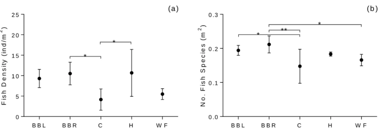
Finally, concerning the reef fish communities, 87 fish species were identified across the 5 reefs. Both density and diversity varies across some reefs (fish density: one-way ANOVA, F4=5.055, p=0.004; fish diversity: one-way ANOVA, F4=5.091, p=0.004, Tukey test, p<0.05) (Figure 3.5a). Carmabi had a lower density than Habitat (Tukey test, p=0.016) and Blue Bay Right (Tukey test, p=0.019). Additionally, it was also less diverse than Blue Bay Left (p = 0.044) and Blue Bay Right (p = 0.003). Water Factory on the other hand had a lower fish diversity than Blue Bay Right (p = 0.049) (Figure 3.5b).

B B L B B R C H W F 0 .0 0 .1 0 .2 0 .3 0 .4 0 .5 N o . o f C le a n in g S ta ti o n s ( m 2 ) S in g le C S P a ir C S T o ta l o f C S B B L B B R C H W F 0 .0 0 .2 0 .4 0 .6 0 .8 1 .0 N o . o f E . e v e ly n a e ( m 2 ) * ** ** ** **

16

Figure 3.5 – Mean (±SD) fish density (a) and fish diversity (b) in the five sampled reefs. Significant differences are

marked with: : * Tukey test, p<0.05; ** Tukey test, p<0.01.Sample size: nBBL= nBBR= nC=nH = nWF=6.

When taking both fish density and diversity into consideration, the fish community was significantly different between all reefs (one-way ANOSIM, R=0.5, p=0.001, pairwise tests p<0.002). In Figure 3.6, one is able to confirm that Carmabi was both separated and showing the highest transect heterogeneity, in opposition to Water Factory which was also separated but more consistent between transects. Blue Bay Left, Blue Bay Right and Habitat look the most similar reefs, showing all the points closer and mostly overlapping each other. Once again the SIMPER analysis identified Carmabi and Water Factory as the reefs with the highest dissimilarity (45.82%).

Figure 3.6 - Multidimensional scaling plot of the fish community across the reefs.

Each point corresponds to a single transect done in each reef. Sample size: 6 transects per reef.

B B L B B R C H W F 0 5 1 0 1 5 2 0 2 5 F is h D e n s it y ( in d /m 2 ) * * (a ) B B L B B R C H W F 0 .0 0 .1 0 .2 0 .3 N o . F is h S p e c ie s ( m 2 ) ( b ) ** * *

17

The frequency of different client species at the single gobies cleaning stations was not significantly different (one-way ANOSIM, R = 0,028, p = 0.186). However for the paired gobies cleaning stations some reefs showed significant differences (one-way ANOSIM, R = 0.159 p = 0.001)1 _{(Table 3.1), with} Water Factory proving to be different to all the reefs (p < 0.05), and Carmabi to Blue Bay Left (p = 0.024) and Blue Bay Right ( p =0.005).

Table 3.1– Total number of client species observed at single and paired cleaning stations

Reef

Single CS

Pairs CS

Blue Bay Left 9 9

Blue Bay Right 9 11

Carmabi 9 9

Habitat 14 7

Water Factory 5 6

3.2. Cleaning goby behavior

3.2.1. Single cleaning gobies

Carmabi was the reef where single gobies had fewer cleaning interactions and Water Factory the reef where cleaning gobies interacted the most, (Kruskal-Wallis H4 = 11.180, p = 0.025, Dunn’s test p=0.021) (Figure 3.7). However, no differences in chases or waiting were observed across reefs (Chases: Kruskal-Wallis H4 = 6.861, p = 0.143; Waiting: Kruskal-Wallis H4 = 3.157 p = 0.532).

Figure 3.7 – Mean frequency of cleaning interactions, cleaner chases and client waits observed

in cleaning stations of single gobies in the five sampled reefs. Significant differences marked with: * Dunn’s test p<0.05

Sample size for all variables: nWF=7, nBBL=nH=9, nBBR=nC=10.2

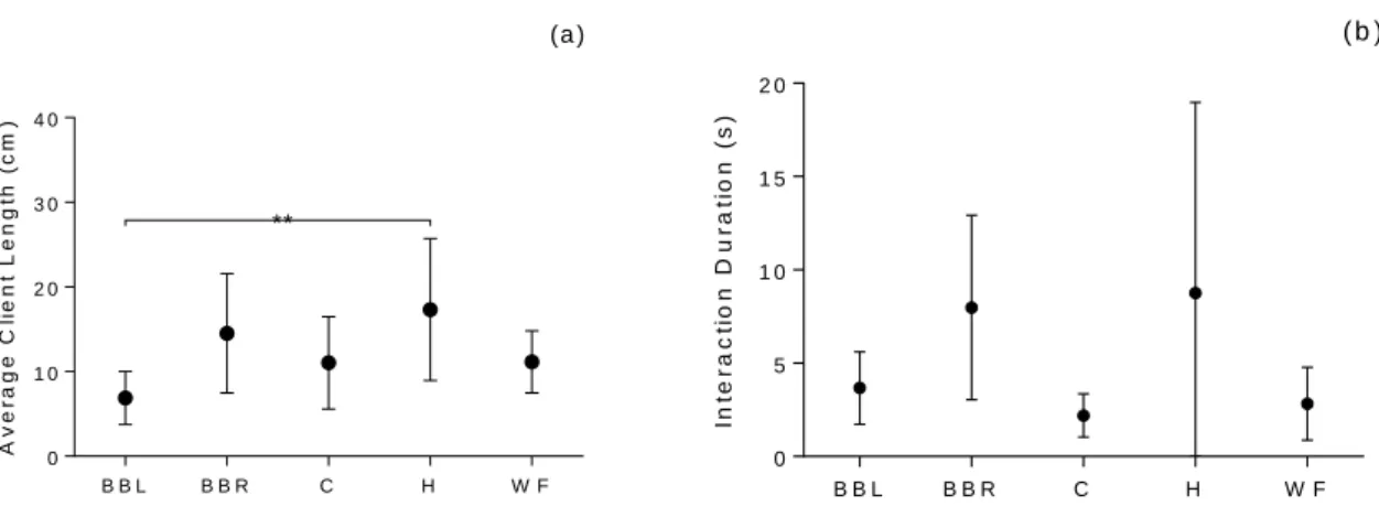
The average length of single cleaning gobies’ clients was in fact different across some reefs (one-way ANOVA, F4 = 3.938, p = 0.009) (Figure 3.8a), however only Blue Bay Left and Habitat were

1 _{The species responsible for these differences can be seen in the form of a Table in Appendix I, p 43.} 2 _{Box-plots of clean, wait and chase frequencies in single CS in Appendix II, p 44.}

B B L B B R C H W F 0 2 4 6 8 1 0 1 2 F re q u e n c y c lie n t w a its c le a n e r c h a s e s c le a n in g in te r a c tio n * *

18

significantly different (Tukey test, p = 0.006), with Habitat (Mean ± SD = 17.32 ± 8.38) having on average bigger clients than Blue Bay Left (Mean ± SD = 6.88 ± 3.13).

Single gobies cleaning interactions had the same duration between reefs (one-way ANOVA, F4 = 1.863 p = 0.148) (Figure 3.8b).

Figure 3.8 – Mean (± SD) average client length (a) and cleaner-client interaction duration (b) at single goby

cleaning stations in the five sampled reefs. Significant differences are marked with: ** Tukey test, p<0.01. Sample size for client size and interaction duration respectively: nWF=7, nBBL=nH=9, nBBR=nC=10; nC=4, nBBL=nH= nWF=6,

nBBR=8.

No significant differences were found across reefs for client likelihood of posing success (Figure 3.9a), (Kruskal-Wallis H4 = 2,927; p = 0,570) the proportion of cleaning interactions initiated by the cleaner (Figure 3.9c) (Kruskal-Wallis, H4 = 6,535; p = 0.163), likelihood of chase by cleaner success (Figure 3.9b) (Kruskal-Wallis, H4 = 1,808 p = 0.771) and client jolts (Figure 3.9d) (one-way ANOVA, F4 = 0.685, p = 0.608). For both likelihood of chase or posing success, the values range from 0 to 2, in this case 0 means that none of the behaviors were recorded, not allowing the calculation of the likelihood. The value 1 is referring to when all poses/chases were rejected, therefore not leading to a cleaning interaction and the value 2 is when all poses/chases lead to a cleaning interaction.

B B L B B R C H W F 0 1 0 2 0 3 0 4 0 A v e ra g e C li e n t L e n g th ( c m ) (a ) ** B B L B B R C H W F 0 5 1 0 1 5 2 0 In te ra c ti o n D u ra ti o n ( s ) ( b )

19

Figure 3.9 - Likelihood of (a) client posing success, (b) chase by a goby success and proportion of cleaning events

that started by cleaner initiative (c) at single cleaning stations. Box-plots represent median, minimum, maximum, 1st and 3rd quartiles. Mean is marked with “+”.

(d) Mean (±SD) jolts per 100s performed by clients at single cleaning goby stations in the five sampled reefs. Sample size for all variables: nWF=7, nBBL=nH=9, nBBR=nC=10.

From the variables described above (jolts/100 s, likelihood of client posing success, likelihood of chase by goby success, proportion of cleaning events initiated by the cleaner and the average interaction duration), only the proportion of cleaning events initiated by the cleaner seemed to be influenced by the reef identity (GLM, distribution = Normal, link function = Identity, p = 0.044). Yet the likelihood of chase by goby success and the proportion of cleaner initiated interactions seemed to be influenced by the average length of the clients positively (GLM, distribution = Normal, link function = Identity, p = 0.006; GLM, distribution = Normal, link function = Identity, p = 0.019, respectively).

3.2.2. Paired cleaning gobies

No differences were found across reefs regarding cleaning or chase frequency (interaction frequency: Kruskal-Wallis, H4 = 6.937; p = 0.139; chase frequency: Kruskal-Wallis, H4 = 2.117, p = 0.714) (Figure 3.10). Significant differences were solely found regarding the waiting frequency (waiting: Kruskal-Wallis H4 = 18.243, p = 0.001). Specifically, these differences were observed between Water Factory and Habitat and Water Factory and Blue Bay Right (Dunn’s test, p = 0.005 and p = 0.023 respectively) where clients were put to wait more frequently (Figure 3.10).

B B L B B R C H W F 0 .0 0 .5 1 .0 1 .5 2 .0 2 .5 L ik e li h o o d o f c li e n t p o s in g s u c c e s s (a ) B B L B B R C H W F 0 .0 0 .5 1 .0 1 .5 2 .0 2 .5 L ik e li h o o d o f c h a s e b y g o b y s u c c e s s ( b ) B B L B B R C H W F 0 2 0 4 0 6 0 8 0 1 0 0 P ro p o rt io n o f c le a n in g e v e n ts s ta rt e d b y t h e c le a n e r ( c ) B B L B B R C H W F 0 2 5 5 0 7 5 1 0 0 J o lt s /1 0 0 s ( d )

20

Figure 3.10 - Mean frequency of cleaning interactions, cleaner chases and client waits

observed in pair cleaning stations in the five sampled reefs. Significant differences marked with * and □, Dunn’s test p<0.05

Sample size for both variables: nH=6, nBBR=7, nBBL=8, nH=nWF=9. 3

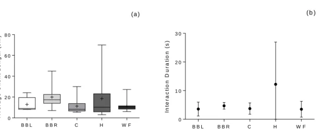
The average length of clients (per reef) and the interaction duration were not significantly different across reefs (average client length: Kruskal-Wallis, H4 = 6.399, p = 0.171; Interaction duration: one-way ANOVA, F4 = 2.158 p = 0.098) (Figure 3.11).

Figure 3.11 – (a) Average length of clients visiting paired cleaning stations in the five sampled reefs. Box-plots

represent median, minimum, maximum, 1st and 3rd quartiles. Mean is marked with “+”. (b) Mean (±SD) duration of cleaning interactions in paired gobies cleaning stations. Sample size for both variables: nH=6, nBBR=7, nBBL=8, nH=nWF=9.

Moreover, no differences were found regarding likelihood of chase by goby success, likelihood of client posing success, in the proportion of cleaning interactions initiated by the cleaner and jolts per 100 s (likelihood of chase by goby success: Kruskal-Wallis, H4 = 2.795 p=0.93; likelihood of client posing success: Kruskal-Wallis, H4 = 6.197, p = 0.185; proportion of cleaner initiated interactions: Kruskal-Wallis, H4 = 3.452 p = 0.474; jolts/100 s: one-way ANOVA, F4 = 1.568, p = 0.208)(Figure 3.12). For

3 _{Box-plots of clean, wait and chase frequencies in paired CS in Appendix III, p 45.}

B B L B B R C H W F 0 2 4 6 8 1 0 1 2 1 4 F re q u e n c y c lie n t w a its c le a n e r c h a s e s c le a n in g in te r a c tio n * * B B L B B R C H W F 0 2 0 4 0 6 0 8 0 A v e ra g e C li e n t L e n g th ( c m ) (a ) B B L B B R C H W F 0 1 0 2 0 3 0 In te ra c ti o n D u ra ti o n ( s ) ( b )

21

both likelihood of chase or posing success, the values range from 0 to 2, in this case 0 means that none of the behaviors were recorded, not allowing the calculation of the likelihood. The value 1 is referring to when all poses/chases were rejected, therefore not leading to a cleaning interaction and the value 2 is when all poses/chases lead to a cleaning interaction.

Figure 3.12 – Likelihood of (a) client posing success, (b) chase by a goby success and proportion of cleaning events

that started by cleaner initiative (c) at paired cleaning stations. Box-plots represent median, minimum, maximum, 1st and 3rd quartiles. Mean is marked with “+”.

(d) Mean (±SD) Jolts per 100 s performed by clients at paired cleaning goby stations in the five sampled reefs. Sample size for all variables: nH=6, nBBR=7,nBBL=8, nC=nWF=9.

None of the variables described above seems to be influenced by reef identity (Jolts/100 s GLM, distribution = Normal, Link function = Identity, p = 0.765; Likelihood of chase success GLM, distribution = Normal, Link function = Identity, p = 0.308; Interaction duration GLM,

distribution = Normal, Link function = Identity, p = 0.203). However the interaction duration was being influenced by the average client size (GLM, distribution = Normal, Link function = Identity, p = 0.003). Models could not be run for the likelihood of client posing success and for the proportion of cleaning events started by the cleaner.

3.3. Diet analysis

Caligids intake in single cleaning gobies stomachs did not vary between reefs (Kruskal-Wallis, H4 = 7.819, p = 0.098) (Figure 3.13a). Gobies also did not cheat differently between reefs (one-way ANOVA, F4 = 0.601, p = 0.667) (Figure 3.13c).The gnathiids on the other hand had significant differences across reefs (one-way ANOVA, F4 = 9.385, p < 0.001) (Figure 3.13b). These differences

B B L B B R C H W F 0 .0 0 .5 1 .0 1 .5 2 .0 2 .5 L ik e li h o o d o f c li e n t p o s in g s u c c e s s (a ) B B L B B R C H W F 0 .0 0 .5 1 .0 1 .5 2 .0 2 .5 L ik e li h o o d o f c h a s e b y g o b y s u c c e s s ( b ) B B L B B R C H W F 0 2 0 4 0 6 0 8 0 1 0 0 P ro p o rt io n o f c le a n in g e v e n ts s ta rt e d b y t h e c le a n e r ( c ) B B L B B R C H W F 0 2 0 4 0 6 0 8 0 J o lt s /1 0 0 s ( d )

22

were observed between Habitat, that had a higher intake of gnathiids, all the other reef (Tukey test, p < 0.05).

Figure 3.13– (a) Number of caligids in single cleaning gobies stomachs and percentage of cheating (c) across five

different reefs. Box-plots represent median, minimum, maximum, 1st and 3rd quartiles. Mean is marked with “+”. (b) Mean (±SD) frequency of gnathiids in single cleaning gobies. Significant differences are marked with: * Tukey test, p<0.05, ** Tukey test, p<0.01. 4

Sample size for all variables: nBBL= nBBR= nC=nH = nWF=5.

The PERMANOVA results showed that the single cleaning gobies stomach content is being significantly influenced by the reef identity (Pseudo-F = 2,660, p = 0.002) (Table 3.2). The pairwise tests revealed significant differences between Habitat and Blue Bay Left, Blue Bay Right and Carmabi (p < 0.05) and between Water Factory and Blue Bay Right and Carmabi (p < 0.05) (Table 3.3).

Table 3.2 - Results of the PERMANOVA analysis conducted to compare the stomach content of single cleaning gobies between

different reefs. Significant p-values (p < 0.05) marked in bold type.

Source

dF

SS

MS

Pseudo-F

P (perm)

Unique Terms

Reef 4 18944 4736 2.6605 0.002 999

Res 20 35602 1780.1

Total 24 54545

4 _{Box-plot of the number of scales found in single gobies in Appendix IV, p 46.}

B B L B B R C H W F 0 5 1 0 1 5 2 0 N o . C a li g id s (a ) B B L B B R C H W F 0 1 0 2 0 3 0 4 0 N o . G n a th id s ( b ) * ** ** ** B B L B B R C H W F 0 2 0 4 0 6 0 8 0 1 0 0 C h e a ti n g ( % ) ( c )

23

Table 3.3 - Results of Pairwise PERMANOVA comparisons between reefs for single cleaning

gobies stomach content (p-values). Significant differences (p < 0.05) in bold type.

Reef

BBL

BBR

C

H

Paired cleaning gobies caligids consumption was similar across all the reefs (Kruskal-Wallis, H4 = 4.306, p = 0.366) (Figure 3.14a), and again, reefs had a similar percentage of cheating (Kruskal-Wallis H4 = 6.678, p = 0.154) (Figure 3.14c). On the other hand, differences across reefs were found for gnathids intake (Kruskal-Wallis, H4 = 12.494, p = 0.014;) (Figure 3.14 b). For gnathiids differences were found between Blue Bay Left and Water Factory (Dunn’s test, p = 0.008), in which the latter had a higher intake than the first.

Figure 3.14 –Number of caligids (a) and gnathiids (b)) in paired cleaning gobies stomachs and percentage of cheating

(c) across five different reefs. Box-plots represent median, minimum, maximum, 1st and 3rd quartiles. Mean is marked with “+”. Significant differences are marked with: ** Dunn’s test, p<0.01.5

Sample size for all variables: nBBL= nBBR= nC=nH = nWF=10.

5 _{Box-plot of the number of scales found in paired gobies in Appendix V, p 46.}

B B L B B R C H W F 0 2 4 6 8 N o .C a li g id s (a ) B B L B B R C H W F 0 2 0 4 0 6 0 N o . G n a th id s ( b ) ** B B L B B R C H W F 0 2 0 4 0 6 0 8 0 1 0 0 C h e a ti n g ( % ) ( c )

24

For paired cleaning gobies stomach content PERMANOVA also demonstrated that these were influenced by the reef identity (Pseudo-F = 2.481, p = 0.008) (Table 3.4) and significant differences were found between all reefs and Water Factory (p < 0.05) and a lack of differences between all the other reefs (all pairwise tests: p > 0.05) (Table 3.5).

Table 3.4 - Results of the PERMANOVA analysis conducted to compare the stomach content of paired cleaning gobies

between different reefs. Significant p-values (p < 0.05) marked in bold type.

Source

dF

SS

MS

Pseudo-F

P (perm)

Unique Terms

Reef 4 20806 5201.5 2.4815 0.008 998

Res 45 94324 2096.1

Total 49 1.1513e5

Table 3.5 - Results of Pairwise PERMANOVA comparisons between reefs for paired cleaning

gobies stomach content (p-values). Significant differences (p < 0.05) in bold type.

Reef

BBL

BBR

C

H

3.4. Cleaning gobies cortisol levels

Single cleaning gobies cortisol levels are significantly higher in Carmabi than in all the other observed reefs (one-way ANOVA, F4 = 6.615, p = 0.001; Tukey test, p < 0.001 for all reefs and Carmabi) (Figure 3.15). These differences were being significantly influenced by the reef where the single gobies lived and the number of client species in their cleaning stations (Table 3.6).

Figure 3.15 –Mean (± SD) cortisol levels in single

cleaning gobies across the five sampled reefs. Significant differences marked with: ** Tukey test, p < 0.01. Sample size: nC=5, nBBL=6, nH=nWF=7, nBBR=8. B B L B B R C H W F 0 1 0 2 0 3 0 4 0 C o rt is o l ( n g /m l) ** ** ** **