Cam design and implementation to a single-cylinder engine to allow for high-altitude operation

(1)

UNIVERSIDADE DA BEIRA INTERIOR

Engenharia

Cam design and implementation to a single-cylinder

engine to allow for high-altitude operation

(Versão revista após discussão)

Francisco Ferreira dos Santos Corrêa Figueira

Dissertação para obtenção do Grau de Mestre em

Engenharia Aeronáutica

(Ciclo de estudos integrado)

Orientador: Prof. Doutor Francisco Miguel Ribeiro Proença Brójo

(2)

(3)

Acknowledgements

I would like to thank everybody who had any implication whatsoever in this project, for without each and every one of them, it would not have been possible, for me, to finish this work.

Firstly, I would like to thank my supervisor, Professor Francisco Miguel Ribeiro Proença Brójo, for all the knowledge, patience, help and guidance shown throughout the development of this dissertation. It would not have been possible without his motivation and constant optimism.

Secondly, to the DCA’s technician and operational assistant, Mr Rui Manuel Tomé Paulo, who had to put up with my constant requests for tools and other materials, always with a smile on his face and still managing to help with the experiment, in the process. When it came to the experimental procedure, I would like to thank Alexandre Nunes for the support, João Rocha for the constant help and great tips, Leonardo Batista and Miguel Calmeiro for the endless days and nights spent at the hangar trying to successfully complete the test runs. Also, to Mara Andrade for putting up with my constant bad mood and still supporting me every day through this journey, to Fábio Morais for the constant support and help through these hard months, and finally to Ana Margarida, Catarina Lopes, David Quintino, Filipe Vinhas, João Prates, and Pedro Dias for all the years they have stayed by my side.

Furthermore, I would like to thank my friends who, throughout the years, formed a second family for me, away from home. Thank you to André Franco, António Lopes, Cátia Miguel, Cátia Moura, Daniel Rodrigues, Daniela Matos, Fabiana Contessoto, Flávia Morais, Gabriel Carrolo, Hélder Gonçalves, Inês Ferrão, Ivo Fernandes, João Morgado, Lídia Lobo, Luís Fialho, Luís Santos, Nídia, Rodolfo Lopes, Rute Neves and all the members of both TEATRUBI and the UBI tennis team.

And last, but certainly not least, to my parents, brother, sisters and every single member of my family for the unconditional support throughout the years, you make me believe that family really does come first, and this journey was certainly made easier due to your presence.

(4)

(5)

Resumo

O design de cames é uma área extremamente complexa e vasta, devido ao facto de ter uma gama de aplicações muito versátil, possível de adaptar para uma grande variedade de sistemas mecânicos. Quando este tipo de estudo é aplicado a motores a pistão, com sistemas de válvulas intrínsecos aos mesmos, podem obter-se resultados muito positivos, ou negativos, tal como fazem os grandes fabricantes da indústria automóvel, que tentam, através da implementação deste tipo de estudos nos seus motores, melhorar o seu desempenho e consumo de combustível. Contudo, no que toca a possíveis sistemas propulsivos para aeronaves não tripuladas (ou UAVs), não existem muitos estudos já feitos acerca deste assunto, devido às condições adversas que estes tipos de motores enfrentam aquando de altitudes elevadas.

O presente trabalho foi feito com o intuito de verificar se é, ou não, possível, adaptar um motor monocilíndrico para funcionar com uma hélice e como meio de propulsão de um pequeno UAV em desenvolvimento pela Universidade da Beira Interior (ou UBI), através da alteração do sistema came-seguidor. O motor selecionado para este projeto, o Honda GX31, é um motor extremamente rotativo e, por isso, o objetivo principal será aumentar o alcance da gama de rotações do motor e mover os picos de binário e potência para regimes de rotação mais baixos, sem sacrificar em demasia esses valores. De forma a atingir esse fim, será necessário alterar o timing das válvulas do motor, através da alteração do próprio perfil da came, devido a este motor ter um sistema came-seguidor muito peculiar, em que apenas uma came controla ambas as válvulas.

No final deste documento são apresentados e discutidos os resultados obtidos experimentalmente, e que levam à conclusão de que é possível ter um grande sucesso nesta área, seguindo os procedimentos relatados nesta dissertação, dado que foi possível aumentar a gama de rotações do motor e reduzir os picos de binário e potência, sem comprometer demasiado os seus valores.

Palavras-chave

(6)

(7)

Abstract

Cam design is a very complex and vast study, due to the fact that its’ applications are very versatile and can be adapted to work with many different mechanical systems. When applied to piston engines comprised of valve trains, this type of study can have a very positive, or negative, impact on the engine’s performance output, like with popular car manufacturers that implement these studies into their engines, in order to enhance their performance and fuel consumption. When dealing with possible Unmanned Aerial Vehicles (or UAVs) propulsion systems, however, not many studies have been done in the past, due to the harsh conditions the engines have to endure at higher altitudes.

The present work tries to assess the possibility of altering the cam-follower system of a single-cylinder engine, in order to adapt it and allow it to work with a propeller, to use as a propulsion system for a UAV in development by Universidade da Beira Interior (or UBI). Due to the fact that the selected engine, the Honda GX31, is a very high-revving engine, the main target would be to broaden the usable power band of the engine and move the maximum torque and power values to lower engine speeds, without compromising those values too much. This should be achieved by altering the valve timing, through alteration of the cam profile itself, since for this particular engine, only one cam lobe controls both the intake and exhaust valves.

At the end of this document, the full experimental results are displayed and discussed, leading to the conclusion that it is possible to have success by following the path this dissertation has carved, since the usable power band was broadened and the reduction in terms of performance output was minimal.

Keywords

(8)

(9)

List of Figures

Figure 2.1 – Adapted cylinder movement schematics for a four-stroke engine [1] ... 5

Figure 2.2 - Cylinder configuration of an SI, four-stroke, DOHC piston engine [2] ... 6

Figure 2.3 - Adapted Theoretical Otto Cycle Diagram (p,V) [4] ... 7

Figure 2.4 - Theoretical Otto Cycle diagram VS Actual Otto Cycle diagram [5] ... 8

Figure 2.5 - Operating cycle of a four-stroke SI engine [1] ... 10

Figure 2.6 - Cross-scavenged designed two-stroke SI engine [6] ... 11

Figure 2.7 - On the left, a crankshaft and camshaft with bucket tappets configuration and, on the right, a crankshaft and camshaft with pushrods and rocker arms configuration [8] ... 12

Figure 2.8 - (a) Radial cam; (b) Wedge cam; (c) Cylindrical cam; (d) Face cam. [9] ... 13

Figure 2.9 – (a) Knife-edge follower; (b) Flat-faced follower; (c) Roller follower; (d) Curved-shoe follower [9]. ... 14

Figure 2.10 - Oscillating follower and the equivalent four-bar mechanism it represents. [10] ... 14

Figure 2.11 - Translating follower and the equivalent four-bar mechanism it represents. [10] ... 14

Figure 2.12 – Adapted representation of the VTEC system, in which (1) is the low rpm operation, (2) is the transition in which the solenoid is being engaged and (3) is the high rpm operation, with all three cams working jointly [13]. ... 15

Figure 2.13 - Simple harmonic motion diagram [14] ... 17

Figure 2.14 - Smoothed curve scatter plots created in the Microsoft Excel software for the 3-4-5-6 polynomial described in this sub-section. ... 22

Figure 3.1 - Scatter point chart of the valve lift measurements, in relation to CA. ... 26

Figure 3.2 - Measured lift curves overlapped with the 3-4-5-6 polynomial motion curves ... 28

Figure 3.3 - Smoothed curve scatter plots for the s-v-a-j diagrams of the 3-4-5-6 polynomial function... 29

Figure 3.4 - Honda GX31 cam-follower system and partial cylinder block. ... 30

Figure 3.5 - Honda GX31 cylinder head and valve train. ... 30

(12)

Figure 3.7 - Representative diagram of the different measurements made in order to dimension the cam profile. ... 33 Figure 3.8 - Smoothed curve scatter plot of the cam profile points, according to R3, the "outer cam

profile" ... 36 Figure 3.9 - Representative diagram of the described process of point translation to create the

actual cam profile ... 37 Figure 3.10 - "Outer cam profile" in blue and the actual Honda GX31 cam profile in black. ... 38 Figure 3.11 – Scatter point chart made with the Microsoft Excel software, depicting the valve lift

measurements made to the new aluminium cam. ... 40 Figure 3.12 - The sixth-degree polynomial alongside the lift measurements. ... 42 Figure 3.13 – Smoothed curve scatter plot of the eight-degree polynomial curves alongside the

measured valve lift curves. ... 46 Figure 3.14 - Smoothed curve scatter plot of the 5-6-7-8 polynomial s-v-a-j diagram according to

equations (3.30-3.33). ... 47 Figure 3.15 - Resulting cam profile from the implemented model. ... 48 Figure 3.16 - Contact of two cylindrical bodies subjected to outside forces [16]. ... 49 Figure 4.1 - Representative diagram of the connections made from the load cell to the Arduino

Nano board [19]. ... 53 Figure 4.2 - Representative diagram of the test stand logic, based on [19]. ... 55 Figure 4.3 – Scatter point plot of the experimental results to show the graphical comparison

between the average torque values of both configurations tested. ... 60 Figure 4.4 - Scatter point plot of the experimental results to show the graphical comparison

between the average power output values of both configurations tested. ... 61 Figure 4.5 - Scatter point plot of the experimental results to show the graphical comparison

between the SFC values of both configurations tested. ... 62 Figure B.1 - CATIAV5 draft of the graduated disk used to measure the valve lift. ... 70 Figure B.2 - Graduated disk, analog dial indicator, articulated arm with a magnetic base and the

Honda GX31 engine attached to the mechanical vice. ... 70 Figure C.1 - Detail of how Rcam varies throughout all the rotation positions. ... 71

(13)

Figure D.1 - Detail of the unviable sharp-pointed cam profile resultant from the implemented model. ... 72 Figure D.2 - Detail of the smooth cam profile resultant from the implemented model that was

supposed to have been manufactured. ... 72 Figure E.1 - Aluminium cam manufactured for the Honda GX31-powered Shell Eco-marathon

vehicle. ... 73 Figure E.2 - Aluminium cam installed in the Honda GX31 and, in the upper-right corner, the original

Honda GX31 cam. ... 73 Figure H.1 - Representative CATIAV5 design of the engine support platform [19]. ... 78 Figure H.2 - Photograph taken of the partial test stand environment, where it is possible to

visualize the components mentioned in Section 4.1.3. ... 78 Figure H.3 - Automotive digital multimeter AT80B on the left and the Hall effect sensor on the

right. ... 79 Figure H.4 - Detail of the throttle cable adapter coupled to the carburettor. ... 79 Figure H.5 - Partial experimental environment and wooden box detail. ... 80 Figure H.6 - Adapted representation of the "T"-shaped tap used to control the fuel flow to the

engine [19]. ... 80 Figure H.7 - Detail of the Hall effect sensor in place, in order to read the magnetic pulses of the

flywheel magnets during the test runs... 81 Figure H.8 - Full test stand configuration (with the exception of the breadboard containing the

(14)

(15)

List of Tables

Table 2.1 - Boundary conditions for a 3-4-5-6 polynomial ... 19

Table 3.1 - Measured valve specifications, according to the CA, for the Honda GX31 ... 26

Table 3.2 - Boundary conditions in order to obtain a 3-4-5-6 polynomial function... 27

Table 4.1 - New cam measured specifications, with the angle values expressed in CA. ... 40

Table 4.2 - Boundary conditions in order to obtain a 5-6-7-8 polynomial function. ... 42

(16)

(17)

Nomenclature

a Acceleration [mm/(º)2_] Cn Constant Coefficients [-] g Gravitational Acceleration Constant [m/s 2_] ḟ Fuel Flow [g/s] j Jerk [mm/(º)3_] L Valve Lift [mm]

L1/4 Valve Lift at ¼ of the duration [mm]

P Power [W]

R1 Length [mm]

R2 Length [mm]

R3 Length [mm]

R4 Length [mm]

Rb Cam Base Circle Radius [mm]

Rcam Cam Radius (variable) [mm]

s Follower Displacement [mm]

SFC Specific Fuel Consumption [g/kW.h]

T Torque [N.m]

(18)

(19)

Greek Symbols

𝛼 Variable Angle [º]

𝛽 Valve duration [º]

δ& Variable Angle [º]

δ' Variable Angle [º]

δ( Variable Angle [º]

δ) Fixed Angle [º]

𝜃 Crankshaft Rotation Angle [º]

𝜎 Contact Stress [Pa]

𝜎,-. Maximum Contact Stress [Pa]

(20)

(21)

List of Acronyms

aBDC aTDC bBDC bTDC BC BEC cA CA CI DOHC DCA DEM DT EEVC EEVO EIVC EIVO EVO EVC GND IVO IVC SFC SI SOHC TDC UAV

After Bottom Dead Center After Top Dead Center Before Bottom Dead Center Before Top Dead Center Boundary Condition Battery Eliminator Circuit Camshaft Rotation Angle Crankshaft Rotation Angle Compression Ignition Double Overhead Camshaft Department of Aerospace Sciences

Department of Electromechanical Engineering Dout

Early Exhaust Valve Closing Early Exhaust Valve Opening Early Intake Valve Closing Early Intake Valve Opening Exhaust Valve Opening Exhaust Valve Closing Ground

Intake Valve Opening Intake Valve Closing Specific Fuel Consumption Spark Ignition

Single Overhead Camshaft Top Dead Center

Unmanned Aerial Vehicle UBI Universidade da Beira Interior

VTEC Variable Valve Timing & Lift Electronic Control

(22)

(23)

Chapter 1 Introduction

1.1 Motivation

In a time where Unmanned Aerial Vehicles (or UAVs) are becoming very popular throughout most sectors of our society, the improvement of propulsion systems that can be used in UAVs is becoming more and more vital. Technology development when it comes to UAV propulsion systems is of vital importance, not only when it comes to jet engines and gas turbines, but also when it comes to regular piston engines that have to be optimized for aerial environments.

Despite the fact that internal combustion engines, or ICEs, have been vastly studied and developed throughout the years since their invention when it comes to improving the performance behaviour of a specific system within the engine, many challenges and obstacles are often found. With the knowledge that UAVs can be used in a wide variety of applications and sectors, finding the adequate propulsion system for any specific case becomes crucial for the further development of these aerial means of transportation.

Having the privilege of studying at Universidade da Beira Interior, or UBI, means that students can get involved in the many projects developed within, and from there comes the main drive of making this dissertation, which aims to verify if single-cylinder engines, like the Honda GX31 and GX35, can be improved, specifically through the alteration of the cam-follower system, to function as a propulsion system for a UAV, to be developed by the Department of Aerospace Sciences, or DCA, within UBI. Many engine manufacturers have developed, throughout the years, systems that enable the variation of the cam-follower systems and drivetrains, in order to improve the engine’s performance, when applied to the automotive industry, however, when it comes to the aeronautical industry, this course of action has not been much pursued, due to the fact that most of the mentioned systems require high engine speeds in order to function efficiently, and with most multi-cylinder, piston engine powered lightweight aircraft, this condition is not met. On the other hand, when it comes to small UAVs, small engines with greater engine speeds can be implemented, with different valve train and cam-follower system configurations, meaning that it is important to, at least, try to verify the viability of using these as propulsion systems.

(24)

1.2 Objectives

The main purpose of the present dissertation is to assess the possibility of broadening the usable power band of a single cylinder piston engine, the Honda GX31, by altering its’ cam-follower system, in order to fit the engine with a viable propeller and use it as a propulsion system for a UAV that is to be developed by UBI. In order to meet this objective, the following tasks were proposed:

Ø Analyse the original cam-follower system, with emphasis on the timing of the valve train and the cam-follower system motion;

Ø Design a new cam profile to meet the desired requirements without largely compromising the engine’s performance;

Ø Manufacture and implement the new cam to the engine and experimentally compare the performance outputs and usable power bands of both the original and new cam configurations.

1.3 Dissertation outline

This dissertation is divided into 5 chapters, with the first and current one including the motivation and objectives.

The second chapter is dedicated to the literature review, in which the operating basics of the piston engine are presented, as well as an in-depth description of the different components of the valve train, their applications and the effect of changing the duration and lift of the valves and the shape of the cam profile. Moreover, an analysis of the complex study of cam design is presented, reasons are given to justify the choice of a specific motion function, with different examples of both more basic functions and very versatile ones.

An analysis of the Honda GX31 cam-follower system is made in the third chapter, in order to endorse the possibility of dimensioning the original cam profile and creating a new one to meet the expected requirements. This chapter is divided into four sub-sections, with the first one describing the procedure that was followed in order to measure the original cam’s valve lift and an analysis of the resulting data, the second one detailing the mathematical method used to derive the needed equations and plot the data, the third one shows the Honda GX31 cam-follower system analysis, detailing the procedure that was followed in order to get the Cartesian coordinates of the original cam profile and finally, the last sub-section was written to elucidate the design of the new cam profile and a brief structural analysis to make sure there is no risk of damaging the engine components upon installation of the new part.

(25)

In the fourth chapter, the experimental components and test run procedures are detailed, as well as the experimental results, discussion and adversities encountered.

Lastly, the fifth chapter includes the dissertations’ conclusions and possibilities for future work on this subject.

(26)

(27)

Chapter 2 Literature review

2.1 Piston engine operating basics

Although there is a very wide variety of piston engine types, we will only focus on reciprocating engines or, in other words, engines in which the piston moves back and forth inside the cylinder, transmitting the power through a connecting rod and crankshaft mechanism to the drive shaft [1] as represented in Figure 2.1. There are also other parameters represented which are important for the comprehension of the piston engine working mechanism, such as:

Figure 2.1 – Adapted cylinder movement schematics for a four-stroke engine [1]

Top-Dead-Centre (TDC), Bottom-Dead-Centre (BDC), bore, stroke, q represents the crankshaft rotation angle, or CA (in degrees), Vd represents the volume that is displaced inside the cylinder, Vc represents the volume inside the combustion chamber and Vt represents the total volume of the cylinder. The ratio between the maximum and minimum volumes is called the compression ratio,

TDC

BDC

(28)

which has typical values of 8 to 12 for spark ignition, or SI engines and 12 to 24 for compression ignition, or CI engines [1].

In order to better understand the working mechanism of the engine, there are other important components worth mentioning, as we can see in Figure 2.2, which is an example of an SI, four-stroke1 piston engine cut view.

Figure 2.2 - Cylinder configuration of an SI, four-stroke, DOHC piston engine [2]

The components shown in Figure 2.2 are briefly described as follows:

Ø Camshaft and Cam - responsible for the opening and closing of the valves and will be

discussed in depth later in the document;

Ø Intake Valve – lets in the air, fuel or mixture, depending on the configuration;

Ø Exhaust Valve – lets the burned mixture out of the cylinder;

Ø Valve Spring – if configured accurately, helps the valves close at the desired timing;

Ø Spark Plug2 - responsible for emitting a spark in order to ignite the air/fuel mixture inside the cylinder;

Ø Combustion Chamber – the portion of the cylinder in which the combustion of the mixture

happens;

Ø Connecting rod – connects the piston to the crankshaft;

Ø Crankshaft – connected to both the driveshaft and the connecting rod, it rotates twice per

cycle in order to move the piston up and down;

1_{Four-stroke engine is one of the classifications given to piston engines, which will be featured in section}

2.2.2.

(29)

Ø Piston – connected to the crankshaft by a connecting rod, it moves up and down in order to

transmit the forces derived from the combustion and pressure inside the cylinder to the crankshaft.

In order to accurately understand the working mechanism of a piston engine, however, we must also introduce the basic thermodynamic concepts behind it. An ICE’s basic principle is to transform the thermal energy, obtained through the chemical reactions of the fuel and air mixture, into mechanical energy, a transformation which occurs according to a thermodynamic cycle. Most ICEs work according to the Otto cycle (which will be described in section 2.2 of this document), but there are other cycles which are worth mentioning like the Diesel cycle, the Miller cycle and the Atkinson cycle.

2.2 Piston engine classification

2.2.1 According to the thermodynamic cycle

2.2.1.1 Otto cycle

One of the most common and known ICE thermodynamic cycles is the Otto cycle, so named after Nikolaus August Otto, who discovered it in 1897 [3]. It is still widely used nowadays when it comes to piston engines, and it’s working process is as follows:

Figure 2.3 - Adapted Theoretical Otto Cycle Diagram (p,V) [4]

In the diagram shown above, we have the following stages: e

(30)

Ø e-c: Isobaric intake (there are no pressure changes while the air enters the intake manifold

and, afterwards, the cylinder);

Ø c-d: Adiabatic/Isentropic compression (there are no heat exchanges with the outside as the

volume decreases and the piston travels up inside the cylinder creating a compression); Ø d-a: Isochoric combustion (there are no volume changes as the pressure increases and the

combustion occurs);

Ø a-b: Adiabatic/Isentropic expansion of the power stroke (there are no heat exchanges with

the outside as the volume increases and the pressure decreases, due to the piston’s downwards movement);

Ø b-c: Isochoric expansion (the exhaust valve opens, there are no volume changes as the burnt

gases exit the cylinder and the pressure decreases);

Ø c-e: Isobaric exhaust (there are no pressure changes while the air leaves the exhaust

manifold).

In Figure 2.3 is described, of course, a theoretical model of the ideal Otto cycle, and doesn’t take into account a lot of variables, such as: both the intake and exhaust phases not being completely isobaric; the combustion not being instantaneous and isochoric; the compression, first and second expansion phases not being adiabatic/isentropic; the third expansion phase not being instantaneous and isochoric and the opening and closing of both the intake and exhaust valves not being instantaneous. Having said this, it’s important to know the differences between the actual Otto cycle representation and the ideal (theoretical) one, as shown in Figure 2.4.

(31)

Even though there are other thermodynamic cycles still used nowadays, they will not be further discussed in this particular document.

2.2.2 According to the work cycle

Piston engines, as a general rule, can be divided into two main categories, when it comes to work cycle3_{: two-stroke and four-stroke engines, and even though their final objective is the same, they} have different working mechanisms and performance results (weight, power output, SFC, etc.). In this section, we will analyse the differences between these two engine categories.

2.2.2.1 Four-Stroke Engines

The vast majority of reciprocating engines operate according to the four-stroke work cycle which means, as the name would suggest, that each cylinder of the engine requires four strokes of its piston (this can also be translated to two crankshaft revolutions) to complete what is known as a full power stroke. This cycle works for both SI and CI engines, and contains the following phases [1] (see Fig. 2.5):

1. An intake stroke, which starts when the piston is at TDC, ends when the piston is at BDC and draws fresh air into the mixture4 along the way. In this phase, and in order to increase the amount of air getting sucked into the cylinder, the intake valve opens shortly before the start of the stroke and closes shortly after its’ end.

2. A compression stroke, that happens when both valves are closed and the piston is moving upwards in the cylinder, compressing the mixture into a small fraction of its original volume. Near the end of this stroke, combustion will be initiated (by means of a spark plug if it’s an SI engine or by means of high compression if it’s a CI engine) and the pressure inside the cylinder sharply rises.

3. An expansion stroke, which starts once the piston is at TDC and the pressure, high-temperature gases push it downwards, forcing the crankshaft to rotate. As the piston approaches BDC (where the stroke will end), the exhaust valve opens to start the exhaust process and force the pressure inside the cylinder to drop.

4. An exhaust stroke, where the remaining burnt gases exit the cylinder through the opening provided by the exhaust valve, due to the difference in pressure inside and outside the cylinder and to the upwards movement of the piston towards TDC. Once the piston

3_{ICEs can be classified according to a lot of different categories, such as ignition type and cylinder configuration.} 4_{Assuming the fuel injection is direct, the injector will send the fuel directly into the cylinder, if it is indirect,}

then the air getting inside the cylinder in the first stroke will already be mixed with fuel, injected into a chamber before the intake valve.

(32)

approaches TDC, the intake valve opens and just after TDC the exhaust valve closes5, starting the cycle again.

Figure 2.5 - Operating cycle of a four-stroke SI engine [1]

2.2.2.2 Two-Stroke Engines

The two-stroke cycle was developed in order to obtain a higher power output from a given engine size with no need for a valve train and, like the four-stroke cycle, can be used with both SI and CI engines.

In this section, we will analyse the simpler form of the two-stroke engine design, in which the ports in the cylinder are opened and closed by the piston movement and control the intake and exhaust flows while the piston is close to BDC (see Figure 2.6)

This cycle contains the following phases [6]:

1. A compression stroke, which begins once the piston covers both the intake and exhaust ports and then compresses the air/fuel mixture while moving towards TDC, point at which the combustion is initiated. As the piston is moving upwards in the cylinder, besides compressing the mixture, it also draws new mixture into the crankcase, through a spring valve.

2. An expansion stroke, which is similar to that of the four-stroke cycle one while the piston approaches BDC, point at which the exhaust port is first uncovered, in order to let the burnt gases out, followed by the intake port, in order to let the air being compressed inside the crankcase to flow through the transfer port and into the cylinder. Both the piston and the ports are shaped so that the fresh mixture doesn’t flow directly out through the exhaust port.

5_{Both the intake and exhaust valves are open at the same time for a short period of time, this phenomenon is}

(33)

In this case, each engine cycle is completed with only one crankshaft revolution, as opposed to the four-stroke cycle. However, it is almost impossible to completely fill the displaced charge with the new mixture, and some of it always ends up flowing directly through the exhaust port.

Figure 2.6 - Cross-scavenged designed two-stroke SI engine [6]

2.3 Camshaft and Valve Train

A camshaft can be described as a rod, comprised with one or more cam lobes (cams), that rotates and slides against a piece of machinery (usually named “follower”) in order to turn rotational motion into linear motion. This change in motion is achieved due to the cam lobes moving closer and further from the axis of rotation, making the follower travel a certain distance, which is called throw or lift [7]. Valve lift is one of the most important variables when it comes to engine performance, due to the fact that it dictates how long the valves stay open for, the amount of overlap6_{between the intake} and exhaust valves, the amount of air, fuel and mixture going in and out of the cylinder, etc.

The working mechanism behind this process is fairly simple: the crankshaft rotates, a timing belt7 makes it possible, through belt tensioners and sprockets, for the camshaft to rotate as well, but with half the crankshaft’s rotational speed. The rotation of the camshaft controls the opening and closing of the intake and exhaust valves, either directly through tappets (Figure 2.7 on the left), or through

6_{Valve overlap happens when both the intake and exhaust valves are open at the same time. This} concept will be explained in more depth further ahead.

7_{A timing belt, belt tensioners and sprockets are one example of the many ways to connect a} crankshaft to a camshaft.

(34)

pushrods and rocker arms (Figure 2.7 on the right) [8]. Seeing as the valves control the amount of air, fuel and mixture going in and out of the cylinder, changing the amount of time that those valves stay open for and/or the point at which they open and close will then change the performance output of the engine itself (SFC, power output, etc.). The process described above of mechanically or electronically manipulating engine valve operations is called Variable Valve Timing (VVT) and it’s a concept that has existed for quite some time now, especially when it comes to the automotive industry, and it is further elucidated in Section 2.5.

Figure 2.7 - On the left, a crankshaft and camshaft with bucket tappets configuration and, on the right, a crankshaft and camshaft with pushrods and rocker arms configuration [8]

2.4 Cam-follower system classification

Usually, the system that links the cam and the follower is known as the cam-follower system or mechanism, and due to the wide range of applications they can be implemented upon, the need to create new geometries, profiles, and mechanisms aroused. This diversity when it comes to designing cam systems also derives from their versatility and flexibility, which leads to a need for a classification to be made [9]. In this section will be mentioned the different classifications given to cam-follower systems, detailing the most used ones, and even though different nomenclatures are given by different authors, one can focus mainly on the classifications given both by Shigley, J. (1981) and by Norton, R. L. (1999).

(35)

2.4.1 According to cam shape

When it comes to cams, they are usually named after their shapes, and the four most usual denominations are: radial cams (Figure 2.8 (a)), wedge cams (Figure 2.8 (b)), cylindrical cams (Figure 2.8 (c)) and face cams (Figure 2.8 (d)). The most common of the mentioned types of cam is the plate radial cam, opposite to the wedge cam, which is not that common, due to the need for a reciprocating movement, not a continuous one [9]. Furthermore, and since the radial cam is the most relevant one for this particular project, we shall henceforth only mention the cam-follower systems that are comprised of radial cams.

Figure 2.8 - (a) Radial cam; (b) Wedge cam; (c) Cylindrical cam; (d) Face cam. [9]

2.4.2 According to follower design

Having mentioned the different types of cams, it is also relevant to mention the different types of followers that have been developed over the years to couple with different cams. As with the previous classification, the follower shape can also be used to classify cam-follower systems, and, like it has been mentioned, only follower shapes that are compatible with radial cams will be discussed. There are four main categories used to classify followers by shape: the knife-edge follower (Figure 2.9 (a)), the flat-faced follower (Figure 2.9 (b)), the roller follower (Figure 2.9 (c)) and the curved-shoe follower (Figure 2.9 (d)) [9]. In the next section, more information will be given as to the different follower motions observed in Figure 2.9, which can also be used to classify, together with the present section, different cam-follower systems.

(36)

Figure 2.9 – (a) Knife-edge follower; (b) Flat-faced follower; (c) Roller follower; (d) Curved-shoe follower [9].

2.4.3 According to follower motion

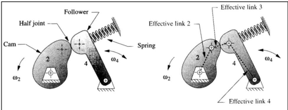
Besides shape and geometry, followers can also be divided into different classifications when it comes to their motion patterns, with the two main groups being: oscillating followers (Figure 2.10) and translating followers (Figure 2.11). Both configurations are equivalents of four-bar mechanisms at any instantaneous position, but with much more versatility and flexibility, due to the fact that, as opposed to rigid four-bar linkages and mechanisms, the “imaginary” linkages in cam-follower systems have different lengths throughout the different rotation positions. [10]

Figure 2.10 - Oscillating follower and the equivalent four-bar mechanism it represents. [10]

(37)

2.5 Variable Valve Timing (VVT)

In this section, a brief explanation of different VVT systems will be given, in order to understand the effects of having different timings and durations when it comes to an engine valve train and cam-follower systems. The first and most primitive form of VVT came into existence in the 19th century, incorporated in steam engines. The early steam locomotives had a system called the Stephenson valve gear, which was able to support variable cut-off of steam admission to the cylinders during the power stroke [11]. Later, and with the evolution of technology, more sophisticated VVT systems were created.

2.5.1 Honda’s VTEC system

Probably one of the best VVT systems of all time, that is still used to this day, is the Honda VTEC (Variable Valve Timing & Lift Electronic Control) system which, appearing in 1990, was definitely the first one to be commercially successful and allowed the manufacturer, at the time, to produce the B16A automotive engine series, comprised of 1600 cm3_{, four-cylinder engines that produced up to} 160 horsepower [12]. These specifications are impressive, even by today’s standards and carved a path through which Honda would come to be very successful. Engines that had the VTEC system (see Fig.2.12), as opposed to other ICEs, were comprised of three cams and three rocker arms for every two (intake or exhaust) valves. Two of those cams are regular ones that operate the valves alone at low engine speeds, optimizing fuel consumption, while the third one is only activated at higher engine speeds (usually 4000-5000 rpm) through a high-pressure oil circuit and a solenoid, working jointly with the other two cams and rocker arms to enhance the engine’s performance, due to the fact that the middle cam is larger than the other two [12]. This means the valves had higher lift and for longer periods of time. As opposed to other car manufacturers, Honda created a system that could vary not only the timing and duration of the valves but also the lift, which was unheard of at the time.

Figure 2.12 – Adapted representation of the VTEC system, in which (1) is the low rpm operation, (2) is the transition in which the solenoid is being engaged and (3) is the high rpm operation, with all three cams

working jointly [13].

(38)

2.6 Cam design curves and diagrams

In this section will be mentioned some of the different ways to create and study cam curves and diagrams, as well as some of the different types that exist and their suitableness when it comes to this particular project. Due to the fact that cam design is a very complex subject, with a lot of different variables and a big mechanical background, an attempt will be made of narrowing it down to the most important concepts for this project without leaving out any crucial information.

When attempting to design a cam profile, some criteria must be met in order for the profile to be suitable for fabrication. First and foremost, it has to obey the fundamental law of cam design and its respective corollary, which state that any cam designed for operation at other than very low speeds must have continuous functions through the first and second derivatives of displacement (velocity and acceleration, respectively) across the entire interval (360 degrees) and also that the jerk function (third derivative of the displacement function) must be finite across the entire interval (360 degrees) [10].

The displacement (s), velocity (v), acceleration (a), and jerk (j) functions mentioned above are crucial when it comes to designing a cam, since they are used to describe the behaviour of the cam--follower system, throughout one revolution of the engine, in which it’s possible to discern a portion of the displacement curve that goes from zero to the maximum lift point (this is called the rise), another that goes from the maximum lift point to zero (this is called the fall or return) and a third portion in which the lift is constant (this is called the dwell) [9].

The s, v, a and j function curves are usually plotted together to form what is called the s-v-a-j diagram, from which it is possible to understand if the cam being studied obeys, or not, the fundamental law of cam design and its corollary, as will be shown in the next sub-section.

2.6.1 Simple harmonic motion curve

One of the most popular curves in the literature is the simple harmonic motion curve. It is one of the standard cam curves and is usually acceptable because the base functions behind it are either sine or cosine functions, which remain continuous throughout any number of differentiations, thus complying with the fundamental law of cam design [10]. The equations for a simple harmonic rise motion are as follows:

s =L 241 − cos(π θ β)> (2.1) v =π β L 2sin(π θ β) (2.2)

(39)

a =π' β' L 2cos(π θ β) (2.3) j = −π ( β( L 2sin(π θ β) (2.4)

where L is the maximum lift, q is the camshaft angle and b is the total angle of the rise segment [9].

After plotting the s-v-a-j diagram for the simple harmonic motion shown in figure 2.88_{, it is clearly} possible to see that the fundamental law of cam design is complied with but, on the other hand, the third derivative is infinite on the nighbouring points of both ends of the curve, which means that the corollary for the fundamental law is not verified.

Figure 2.13 - Simple harmonic motion diagram [14]

Despite the fact that the simple harmonic motion curve can seem appealing due to the fact that some of the fundamental criteria are easily met, the corollary of the fundamental law of cam design is not met and the second derivative of the displacement isn’t zero at the beginning and ending of the motion. What this means is that this motion curve cannot be used (at least by itself) to accurately predict the behaviour of the cam-follower system and is, therefore, not suitable for high-speed movements. In the next section will be mentioned the combined motion curves, with the main goal being to reduce the acceleration values and variations in order for the cam to be reliable and not damage any engine components during rotation. These combined motion functions may also prove to be more accurate than the standard ones.

8_{It is possible to observe that the nomenclature used by Rothbart, Harold A. (2004) indicates that instead of}

(40)

2.6.2 Combined functions

Combined motion functions are usually appealing to cam designers due to the fact that they combine diverse basic motion functions into one, meaning it is more accurate and less likely to fail the strict cam design criteria, while still having some adjacent simplicity to them. As a general rule of thumb, when designing a cam, one must focus on reducing the acceleration values and their variation, and from this comes the modified trapezoidal acceleration. This function is a combination of both the sine acceleration curve and the constant acceleration one, which means that a full period sine wave is “cut” into fourths and “placed into” the square, constant acceleration curve, which creates a smooth transition from the functions’ zeros to the maximum and minimum values of the function) [10].

There is a wide variety of combined functions the cam designer can choose from, however, for the sake of reducing the document size, these will not be deduced and specified in this particular document, also due to the lack of interest of these functions for this specific project.

2.6.3 Polynomial functions

Although the standard and combined cam functions mentioned before (and a wide variety of others) are usually adequate if accurately dimensioned, they certainly don’t represent the whole picture when it comes to cam design functions. It is often common to opt to create polynomial motion curves, due to the fact that these are very versatile and can, therefore, be tailored to the designer’s wish [9]. The general form of the polynomial motion equation is as follows:

s = CF+ C&x + C'x'+ C(x(+ C)x)+ CIxI+ CJxJ+ ⋯ + CLxL (2.5)

with s being the follower displacement, x being the independent variable which, in our case, is going to be q/b, and finally Cn being the unknown constant coefficients which will be found to fulfil the requirements of a specific design [10]. The degree of the polynomial function to be used is going to be determined by the number of boundary conditions (or BCs) specified at the beginning of the design process with the following relation:

n = BCN_{s − 1} _(2.6)

where the BCs will be specific points, chosen by the designer, throughout the s-v-a-j diagram in order to tailor the resulting curves to the desired end.

Since the BCs are going to be the parameters that dictate the number of variables of the polynomial equation, the first step to accurately create the desired curve is to specify the BCs keeping in mind

(41)

the final objective. As an example, As an example, a 3-4-5-6 polynomial function will be created by using two segments of BCs, one for the rise-fall (q = 0 and q = b) and another for the dwell (q = b/2), as in Table 2.1:

Table 2.1 - Boundary conditions for a 3-4-5-6 polynomial

Position of q according to b Boundary Conditions

q = 0 s=0 v=0 a=0

q = b/2 s=L

q = b s=0 v=0 a=0

which means, by having 7 BCs, according to equation (2.6), the polynomial equation to be created will have a degree of 6, is the aim of in this example. If the independent variable is then replaced in equation (2.5) for q/b, the latter becomes:

s = CF+ C&O θ βP + C'O θ βP ' + C(O θ βP ( + C)O θ βP ) + CIO θ βP I + CJO θ βP J (2.7)

and consequently, the first, second and third derivatives become:

v = 1 βQC&+ 2C'O θ βP + 3C(O θ βP ' + 4C)O θ βP ( + 5CIO θ βP ) + 6CJO θ βP I V (2.8) a = 1 β'Q2C'+ 6C(O θ βP + 12C)O θ βP ' + 20CIO θ βP ( + 30CJO θ βP ) V (2.9) j = 1 β(Q6C(+ 24C)O θ βP + 60CIO θ βP ' + 120CJO θ βP ( V (2.10)

keeping in mind that, since the jerk is not constrained in the boundary conditions, it won’t be necessary to use equation (2.10) to find the constant coefficients.

Having found the necessary derivatives, then one has to substitute the BCs shown in Table 2.1 in equations (2.7), (2.8) and (2.9) in order to solve for the constant coefficients. Starting with the first set of BCs specified:

q = 0 s=0 v=0 a=0

it can be seen firstly that when q=0, s=0 and as so, by substituting these values in equation (2.7), one obtains:

(42)

0 = CF+ C&O 0 βP + C'O 0 βP ' + C(O 0 βP ( + C)O 0 βP ) + CIO 0 βP I + CJO 0 βP J ⇔ ⇔ CF= 0 (2.11)

therefore, by repeating this process for v=0 in equation (2.8) and a=0 in equation (2.9), the results are respectively: 0 =1 β4C&+ 2C'( 0 β) + 3C(( 0 β)'+ 4C)( 0 β)(+ 5CI( 0 β))+ 6CJ( 0 β)I> ⟺ ⟺ C&= 0 (2.12) and 0 = 1 β'42C'+ 6C(( 0 β) + 12C)( 0 β)'+ 20CI( 0 β)(+ 30CJ( 0 β))> ⟺ ⟺ C'= 0 (2.13)

and so, after analysing the first set of BCs, the values of the first three constant coefficients are obtained.

Only four unknown coefficients remain, and the previous calculation process will be repeated for the last set of four BCs, in order to obtain four new equations to solve simultaneously:

q = b/2 s=L

q = b s=0 v=0 a=0

Substituting the first BC in equation (2.7) gives:

L = C(( 1 2)(+ C)( 1 2))+ CI( 1 2)I+ CJ( 1 2)J⟺ ⟺ L = C(1 8+ C) 1 16+ CI 1 32+ CJ 1 64 (2.14)

and repeating the same process for the last three BCs, when q = b, in equations (2.7), (2.8) and (2.9) respectively:

(43)

⟺1

β(3C(+ 4C)+ 5CI+ 6CJ) = 0 (2.16)

⟺ 1

β'[6C(+ 12C)+ 20CI+ 30CJ] = 0 (2.17)

Finally, having found four equations to solve for the four unknown constant coefficients, with resource to any calculator or computer that contains a matrix solving function, it is possible to find the four coefficients simultaneously, by putting equations (2.14), (2.15), (2,16) and (2.17) into a matrix and solving for the unknown coefficients:

⎣ ⎢ ⎢ ⎢ ⎡ 1 8 1 16 1 32 1 64 1 1 1 1 3𝓍 4𝓍 5𝓍 6𝓍 6𝓍' _12𝓍' _20𝓍' _30𝓍'_⎦⎥ ⎥ ⎥ ⎤ d C( C) CI CJ e = d L 0 0 0 e , with 𝓍 =1 β j C(= 64L C)= −192L CI= 192L CJ= −64L , with β ≠ 0

Since the first three constant coefficients were already known from equations (2.11), (2.12) and (2.13), the 3-4-5-6 polynomial and its’ three derivatives can now be obtained by substituting the constant coefficients in equations (2.7), (2.8), (2.9) and (2.10):

s = L Q64(θ β)(− 192 O θ βP ) + 192 Oθ βP I − 64 Oθ βP J V (2.18) v = L βQ192( θ β)'− 768 O θ βP ( + 960 Oθ βP ) − 384 Oθ βP I V (2.19) a = L β'Q384 O θ βP − 2304 O θ βP ' + 3840 Oθ βP ( − 1920 Oθ βP ) V (2.20) j = L β(Q384 − 4608 O θ βP + 11520 O θ βP ' − 7680 Oθ βP ( V (2.21)

(44)

The plot of these four equations, considering b=360º, qÎ[0º;360º] and L=3mm9_{is presented at Fig.} 2.14.

In Figure 2.14 it is possible to graphically confirm that there are no discontinuities in the displacement, velocity and acceleration functions and that the jerk function is finite throughout the entire interval, thus confirming that both the fundamental law of cam design and its’ corollary are complied with.

Although there is a very wide variety of functions to choose from, including even more versatile versions of the polynomial functions mentioned in this subsection, called spline functions [14], due to the fact that for this particular project they have no interest, the criteria and derivation procedure will not be specified like for the polynomial functions. Furthermore, it’s important to note that polynomial functions can accurately predict the behaviour of the cam-follower system at the BCs but, there is no telling if they will have the desired behaviour in between those points. This is

9_{These are only example values; all of the mentioned variables can have whichever values the} designer requires.

Figure 2.14 - Smoothed curve scatter plots created in the Microsoft Excel software for the 3-4-5-6 polynomial described in

(45)

especially true for higher degree polynomials, which is why the best approach when attempting to find an accurate function is to try and minimize the number of BCs used for the curves to fit the designer’s needs.

(46)

(47)

Chapter 3 Cam Design

3.1 Valve lift measurement

In order to accurately dimension the new cam, the first step is to get to know the original one of the Honda GX31 (the full engine specifications can be found in Table A.1 of Appendix A), which means a study about the valve lift, velocity, acceleration and jerk will have to be made.

When it comes to the valve lift, a practical approach has been taken, with the experimental procedure being as follows:

Ø Firstly, a graduated disk was created, utilizing the software CATIAV5 (Fig. B.1 of Appendix B), in which the scale was from 0º to 360º10, with 2º intervals;

Ø The disk was then printed and coupled to a round, wooden plank which was, afterwards, perforated with a drill in order to couple the disk to the engine through means of two screws; Ø The engine is then locked in place by a mechanical vice and the disk coupled to the engine ; Ø When coupling the disk to the engine, it’s important to make sure the 0º mark is coincident with the TDC (which can be easily located by removing the spark plug and checking when the piston is at the top of the cylinder before the exhaust valve opens and then align a little cut on one of the flywheel fins with a metallic pin on the cylinder block, and it’s also important to pinpoint the location which is used as a reference for the degree measurement, when rotating the flywheel and the disk;

Ø Once the engine is locked in place, the valve cover is removed in order to reach the rocker arms and, through means of a feeler gauge, both the intake and exhaust valve clearances are set according to the manufacturers’ specifications (Table A.1 of Appendix A);

Ø The next step in the process is, still keeping the valve cover removed, to mount the valve lift measuring apparatus, which consists of a magnetic-based mechanical arm, placed at the base of the mechanical vice, and an analogical dial indicator mounted on the non-magnetic end of the mechanical arm with the probe tip resting on the valve spring. Since the dial indicator will be used to measure the amount of valve displacement (lift), it’s important to make sure it is completely vertical to minimize the measurement errors;

Ø Once the apparatus is fully mounted and functional (see Figure B.2 of appendix B), the measurements start taking place, beginning with the intake valve. With the disk set at 0º, it is then slowly rotated, by hand, anti-clockwise and once the first movement is seen on the

(48)

dial indicator, the value of the lift is written down, that point is considered to be the IVO and from that point onwards, every 2º increment results in a valve lift change, which is written down. This process continues until the valve lift reaches 0 mm again, this point is considered to be the IVC and marks the end of the measurements for the intake valve lift; Ø The latter process is repeated for the exhaust valve and this means that all the measured

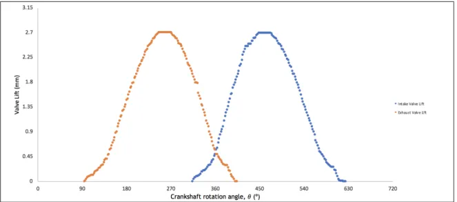
values can be plotted into a scatter point chart in the Microsoft Excel software, giving a rough approximation of the valve lift curves (Figure 3.1).

Figure 3.1 - Scatter point chart of the valve lift measurements, in relation to CA.

In the valve displacement chart displayed in Fig. 3.1, it’s possible to observe some unusual characteristics when it comes to measurement precision. Firstly, it’s important to recognize that the analogic dial indicator used is a very sensitive piece of equipment, due to the fact that the scale is so small (maximum of 10 mm with 0,1 mm intervals) and what this means is that, even though the procedure has been carried out with extreme care to avoid any lack of precision, any small disturbance to the apparatus environment will cause a less accurate measurement. Furthermore, the lack of precision seen is also caused by a compression release mechanism incorporated to the camshaft that is used to ease a cold starting of the engine, by raising the follower through means of a machined metal pin, not letting the exhaust valve close under a certain engine speed, and therefore releasing the compression inside the cylinder so that the engine can start without having to work against the pumping of the piston.

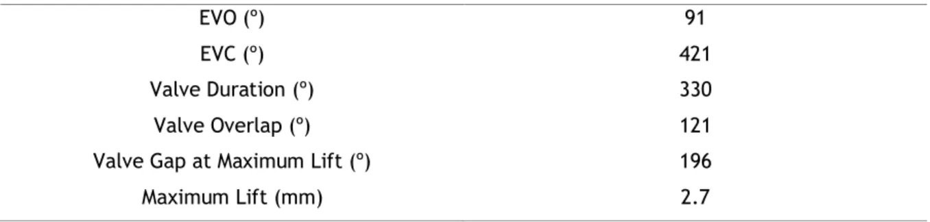
Table 3.1 shows the values that can be read in the plotted measurements in Figure 3.1.:

Table 3.1 - Measured valve specifications, according to the CA, for the Honda GX31

IVO (º) 300

IVC (º) 63011

11_{Due to the measurement imprecisions mentioned in this section, the values of both the IVC and} EVC were read in the polynomial approximation curve shown in the next section.

(49)

EVO (º) 91

EVC (º) 421

Valve Duration (º) 330

Valve Overlap (º) 121

Valve Gap at Maximum Lift (º) 196

Maximum Lift (mm) 2.7

3.2 Lift curve approximation and s-v-a-j diagram

In this section will be mentioned the procedure that was followed in order to solve and plot the polynomial equation that follows approximately the same pattern as the measured lift curve, shown in the prior section of this chapter. As it has been in Chapter 2, there is a wide variety of curves that can be used to describe valve movements in ICEs, and it’s usually possible to simply adapt those curves to the desired situation by changing the BCs of the system. In this case, however, it was decided that a new curve should be created for the lift (and consequently the velocity, acceleration and jerk) since this would mean that the full range of the curve (rise, fall and dwell) could be incorporated into a single set of equations.

The process for the creation of the polynomial motion curve is the same that was demonstrated in Section 2.5.3 of this dissertation, with the exception of the values of b which will be equal to the valve duration shown in Table 3.1 (b=330º), q which will range from the beginning to the end of the valve duration interval (qÎ[91º;421º] for the exhaust valve and qÎ[314;644º] for the intake valve) and the maximum lift which will be equal to the measured one (L=2,7mm). The first step is to define the BCs as it was done in Section 2.6.3:

Table 3.2 - Boundary conditions in order to obtain a 3-4-5-6 polynomial function

Position of q according to b Boundary Conditions

q = 0 s=0 v=0 a=0

q = b/2 s=L

q = b s=0 v=0 a=0

which, as it’s possible to observe in Table 3.2, are exactly the same as Table 2.1, since the constraints desired for this polynomial function are the same as the one used as an example in Section 2.5.3. What this means is that the final motion equations will be the same as equations (2.18-2.21) which will then be modified to fit the measured values of this specific system and, if the resulting displacement curve doesn’t adapt accurately to the measured curves in Figure 3.1, one must keep adding BCs until the resulting curve is satisfactory. Having said this, the values of b and L are substituted in equations (2.18-2.21), obtaining:

(50)

s = 2,7 Q64 O θ 330P ( − 192 O θ 330P ) + 192 O θ 330P I − 64 O θ 330P J V (3.1) v = 2,7 330Q192 O θ 330P ' − 768 O θ 330P ( + 960 O θ 330P ) − 384 O θ 330P I V (3.2) a = 2,7 330'Q384 O θ 330P − 2304 O θ 330P ' + 3840 O θ 330P ( − 1920 O θ 330P ) V (3.3) j = 2,7 330(Q384 − 4608 O θ 330P + 11520 O θ 330P ' − 7680 O θ 330P ( V (3.4)

and, since the values of q range from the EVO to the EVC, for the exhaust valve, and from the IVO to the IVC, for the intake valve, the motion curves can be plotted (see Fig. 3.2) together with the measured curves, in order to understand if this sixth-degree polynomial adapts to the measurements.

Figure 3.2 - Measured lift curves overlapped with the 3-4-5-6 polynomial motion curves

After having plotted the sixth-degree polynomial curves over the measured ones, it can be seen that they adapt well, albeit not completely accurately, but still accurate enough to avoid having to use a higher-degree function that may cause undesired variations in the motion behaviour. There is still need, however, to verify that the profile of the derivatives is within the acceptable threshold (see Fig. 3.3).

(51)

Figure 3.3 - Smoothed curve scatter plots for the s-v-a-j diagrams of the 3-4-5-6 polynomial function

Having plotted the complete s-v-a-j diagram, it can be confirmed that the first and second derivatives are continuous throughout the entire measured interval and that the third derivative is finite throughout the same interval. This means that the polynomial motion function derived in equations (3.1-3.4) can be used to describe the motion behaviour of this particular cam-follower system.

In the next section, the design of the cam-follower system mechanism will be presented, which will be used to allow the creation of a cam profile in the Microsoft Excel software.

(52)

3.3 Cam-follower system analysis

As was demonstrated in Section 2.4, there is a wide variety of cam-follower systems available for manufacturers to choose from when conceiving engines or other mechanisms that involve the use of camshafts and followers. However, the cam-follower system in the Honda GX31 is a very unusual and distinctive one, in the sense that it’s a mixture of a few different mentioned systems with some unusual characteristics. For this reason, a detailed description of the system’s working mechanism will be made and, later in the section, the procedure followed for the creation of the cam profile will be shown and explained.

Next, some photographs will be shown in which it is possible to see the actual mechanism present in the Honda GX31 engine, with a legend to discern each of the crucial components (see Figs. 3.4 to 3.6).

The components shown in Figures 3.4 and 3.5 are as follows:

Ø A – Cam lobe and spur gear that connects to the crankshaft;

Ø B – Followers (for the exhaust valve on the left and for the intake valve on the right);

Ø C – Pushrods that connect the followers to the rocker arms (the one furthest away for the

exhaust valve and the one nearest for the intake valve);

Ø D – Rocker arms that translate the follower motion to the valves (the one furthest away for

the exhaust valve and the one nearest for the intake valve);

Figure 3.4 - Honda GX31 cam-follower system and partial cylinder

block.

Figure 3.5 - Honda GX31 cam-follower system and partial cylinder

block.

Figure 3.5 - Honda GX31 cylinder head and valve train.

Figure 3.6 - Honda GX31 cylinder head and valve train.

A A B B D D F F E E C C

(53)

Ø E – Intake valve spring (the exhaust valve spring can’t be seen in this picture but it’s directly

below the exhaust valve rocker arm);

Ø F – Intake valve (the exhaust valve can’t be seen in this picture but it’s directly below the

exhaust valve rocker arm);

Whereas the components shown in Figure 3.6 are as follows:

Ø G – Crankshaft bearings;

Ø H – Piston;

Ø I – Connecting rod;

Ø J – Crankshaft;

Ø K –Engine flywheel;

Ø L – Spur gear that rotates with the flywheel and connects to spur gear shown in A, making it,

and consequently the cam lobe, rotate clockwise; Ø M – Oil dipstick used to check the engine oil level;

Ø N – Oil pan.

As it is shown in Figure 3.4, there are some unusual characteristics when it comes to this particular cam-follower system: first and foremost, there is a single, egg-shaped cam that controls, through oscillating, curved followers, both the intake and exhaust valves. When it comes to designing a new cam for the engine, this can prove to be a difficult obstacle due to the fact that trying to alter the behaviour of one of the valves will, consequently, alter the behaviour of the other one i.e., if the cam is designed in order to achieve EIVC the first thing to happen is that EEVC is also obtained (which

Figure 3.6 - Honda GX31 top-view of the block internal components.

H K I M N J G L

(54)

can be prejudicial in the sense that when the intake valve opens again, there will be residual burned gases still inside the cylinder). The other eventually that will occur is that if only one aspect of the cam-follower mechanism behaviour is altered, an asymmetrical cam profile will be obtained as a result and although this is not unheard of in the cam design subject, it is not usually favourable.

Having said this, the actual geometrical analysis of the system will be presented, in which the first step is to try to photograph the mechanism with a nearby scalar instrument to serve as a benchmark for the image’s scale12_{, then enlarge the image and print it, so that it is possible to determine the} necessary constraints for the designing of the cam profile.

In Figure 3.7 is shown the mentioned image with the measured constraints and variables, in which, when it came to the measurement of the different angles and distances, R1, R2, R3, R4, Rb, j and d4 were measured using the suitable instruments (Rb was measured directly on the cam with the aid of a Vernier Calliper while j, d4 R1, R2, R3 and R4 were measured on the enlarged photograph using a digital protractor and a graduated ruler) and, when it came to the distances, all of them were measured in millimetres and divided by 6,8 in order to adapt to the chosen scale, while the angle was measured in degrees. Keeping this in mind, R1 was considered to be the distance between the centre13_{of the follower locking pin and the position of the base of the intake valve pushrod (which} had been removed at the time the photograph was taken), R2 the distance between the centre of the follower locking pin and the centre of the follower circumference arc depicted in Figure 3.7 (point O), R3 the distance between the centre of the cam locking pin and point O, R4 the distance between the centre of the cam locking pin and the centre of the follower locking pin, Rb the radius of the cam base circle and, finally, j and d4 are constant values that are considered to be the angle between R1 and R2, and between R4 and the imaginary horizontal axis that crosses the centre of the cam locking pin, respectively.

12_{The scale presented in Figure 3.7 represents the actual scale read when taking the system’s measurements}

and not the scale that can be seen in this document.

13 _{Since the photograph was not exactly centred, the actual centroid of the pin face is deviated, as shown in}

(55)

Figure 3.7 - Representative diagram of the different measurements made in order to dimension the cam profile.

The measured values are as follows:

R&= 93,8 6,8 = 13.8 mm R'= 240 6,8 = 35.3 mm R)= 206,7 6,8 = 30.4 mm Rq= 10 mm φ = 8.7° δ)= 90°

Although the values shown above will be the basis of the design, there are still some unknown variables, starting with R3 which was not specified as a fixed value like the rest of the measured distances. This is due to the fact that R3 varies with the cam radius which, in the case of Figure 3.7 is equal to Rb, but when the cam rotates to other positions, will have different values because of the “nose” seen in Figure 3.4 (see Fig. C.1 of Appendix C), i.e. the enlarged photograph depicted in Figure 3.7, allowed for the measurement of one R3 value, which is:

R(=226 6.8+ 10 = 43.2 mm 1:6,8 [cm] R4 R1 R2 R3 R_b º R_ca m O 𝛿' 𝛿( 𝜑 𝛿) 𝛿&

(56)

which is an approximated value and, for this reason, further ahead an equation to solve for all the values of R3 is deducted and those are the values used when designing the cam.

Having said this, and before mentioning the rest of the variables shown in Figure 3.7, such as d1, d2 and d3, it is very important to understand the logic behind the dimensioning presented in this section. What is happening is that it is being considered that the whole system represented in Figure 3.7 rotates around the cam, following the represented dashed trajectory passing through point O, with the result being that this trajectory, once a full cycle is completed, will represent an enlarged version of the actual cam profile, which will afterwards be reduced to its’ actual size. To achieve this, there are three variables that have to be used, besides the ones that were already mentioned, and they are d1, d2 and d3, which represent different angles that vary throughout the entire cycle. They are intricately related to the remainder of the mentioned variables and constants, as follows:

δ&= 𝑠

𝑅& (3.5)

δ'= δ&− φ (3.6)

with s being the follower displacement values from equation (3.1) for each angular position and, in order to simplify the next part, the value of d4 will be displayed in radians (instead of having δ)= 90°, we shall have δ)=

w ' rad):

R(

zzzz⃗ = Rzzzz⃗ + R) zzzz⃗ ⟺ '

⟺ R(e}.~• _{= R)e}}.~€_{+ R'e}}.~• _⟹

~_€ƒw ' „……† R(e}.~• = R)e}. w '+ R_'e}.~• ⟺ ⟺ R(e}(~•‡ w ')= R₎e}.F+ R_'e}(~•‡w_')_⟺

Separating the real and imaginary parts into a system of equations:

jR(cos ˆδ(− π 2‰ = R)+ R'cos ˆδ'− π 2‰ R(sin ˆδ(− π 2‰ = R'sin ˆδ'− π 2‰ ⟺ (3.7) ⟺ jR( '_cos'_ˆδ (− π 2‰ = R)'+ 2R)R'cos ˆδ'− π 2‰ + R''cos'ˆδ'− π 2‰ R('sin'ˆδ(− π 2‰ = R' '_sin'_ˆδ '− π 2‰ (3.8)