Adding detailed transmission constraints to a long-term integrated
assessment model – a case study for Brazil using the TIMES model
Raul Miranda
a 1, Sofia Simoes
b, Alexandre Szklo
a, Roberto Schaeffer
aa Energy Planning Program, Graduate School of Engineering - Technology Center, Universidade Federal
do Rio de Janeiro, 21941-972 Rio de Janeiro, Brazil
b CENSE – Center for Environmental and Sustainability Research, NOVA School of Science and
Technology, NOVA University Lisbon 2829-516 Caparica, Portugal.
Abstract
Onshore wind and solar-photovoltaic-based electricity are expected to drive most of the global growth in renewable energy sources capacity until 2020. This creates a challenge for properly modelling such intermittent variable resources since: (i) their availability varies spatially and temporally and (ii) thus, their integration in power systems is determined by the configuration of transmission grids. Large energy system models usually adopt simplified approaches for modelling wind and solar photovoltaic (PV) deployment and the power grid. This paper uses the recently developed TIMES-Brazil optimization model to study the role of transmission bottlenecks in cost-effective long-term deployment of wind and solar power in the Brazilian energy system up to 2050. The model explicitly models the grid infrastructure of 29 regions in Brazil differentiated according to existing power plants, wind and solar availabilities, future RES potentials and power demand. Three different scenarios (Free Trade, Simplified Trade and Detailed Trade), with increasingly more detail in modelling electricity transmission lines, were tested. Findings show that a more detailed transmission infrastructure significantly affects capacity deployments and electricity prices. The grid connecting the North and South of Brazil was found to be the most important bottleneck affecting the deployment of solar in the country.
1 Introduction
The contribution of onshore wind- and solar-photovoltaic (PV)-based electricity are expected to drive most of the global growth in renewable energy sources (RES) capacity until 2020 [1]. This increase in wind and PV electricity is motivated not only by their cost reductions, but also by policies aiming to foster energy security, to reduce greenhouse gas (GHG) emissions and to improve air quality [2].
However, the generation potential and integration possibilities for variable intermittent RES as wind and solar depend on geographic characteristics [3–7]. Moreover, large-scale deployment of wind and solar is frequently constrained by the existing transmission and distribution grid infrastructure [5,8]. Consequently, modelling expansion pathways of such RES energy technologies can be made more accurate by considering spatial and temporal variability of the resources across the modelled energy system, as well as the existing electricity grid bottlenecks [9–12]. Challenges due to their integration are also dependent on existing power plants and their locations [13]. In Brazil, although the current hydro capacity is scattered along the country, the remaining expansion potential is predominantly located in the north of the country in an environmentally-sensitive area. The load demand in turn is mostly located in the southern part of the country. In 2017, around 70% of the Brazilian installed capacity was made up by hydropower, 7% by wind turbines and the remaining by thermal units, while solar projects were still incipient [14].
Global or national energy system models as TIMES [15], MESSAGE [16,17] or PRIMES [18] integrate the several components of the system from resource extraction, to conversion into energy carriers and to end-use consumption. Due to difficulties in obtaining the necessary data and the increased computational complexity, such models often have a simplified temporal (e.g. an average year is divided in a low number of representative time-slices) and geographical resolution (e.g. countries are represented as one aggregated region) [8,18–21]. Subsequently, electricity transmission processes are frequently modelled as only one node per country and wind and solar variability is assumed to be homogeneous throughout the modelled system. Such simplified approach does not allow to consider the differences within a country regarding electricity demand, different wind and solar availabilities throughout the terrain and the year, and grid bottlenecks affecting the transmission large volumes of intermittent variable electricity within a country [8,22]. This is particularly relevant for large countries such as Brazil.
To our knowledge, this is the first-time grid processes and bottlenecks are assessed in such detail using an energy system model. Although similar work has been done using power system models, the same has not been done with TIMES considering a very detailed representation of nodes and processes. Because of this, it is possible in this paper to: 1) assess the significance of grid
bottlenecks and 2) test different levels of detail in modelling grid processes in energy system models. This allows providing innovative insights on the best possible trade-off between accurate representation of reality (in this case electricity transmission) and increased computation time. There has been substantial literature studying the role of wind and solar electricity in the Brazilian energy system. For example, [23] focused on the deployment of Concentrated Solar Power (CSP) up to 2050; [16] used an ensemble of six energy models to study decarbonisation scenarios for Brazil up to 2050 and found that decarbonisation of the power sector was mostly due to the use of biomass, solar and wind; [24] used a simulation model in combination with the optimisation model MESSAGE to assess policy incentives to foster solar deployment in Brazil up to 2040; [25] used the LEAP simulation model to develop scenarios till 2030 and estimate that wind and solar power shall increase; and [26] applied a Multi-Criteria Assessment tool to study 5 power system scenarios for Brazil up to 2050 and concluded that the scenario with largest contribution from wind and biomass was the preferable option.
These studies either focused on simulation approaches or did not consider spatial disaggregation in the optimisation tools used. Moreover, these studies did not address the role of transmission bottlenecks in the developed scenarios for the Brazilian power system. Some authors have considered the role of the transmission infrastructure. For example, [27] considered energy transmissions between three Brazilian macro regions, not taking into account internal boundaries within those regions. A similar approach considering only the northeast region was made by [28]. A more transmission-detailed approach was made by [29] applying the REMix model to test the role of wind and solar power, as well as transmission lines in a 100% renewable energy system in Brazil by 2050. The model was used to find the least-cost solution associated with expansion and operation, given the target of a fully renewable electric power system.
In this context, we take the approach of [27], [28] and [29] a step further. Our study can be seen as complementary as our aim is to assess the role of transmission bottlenecks in cost-effective long-term deployment of wind and solar power in the Brazilian energy system up to 2050. Regarding [29], for instance, there are a few comments we could engender. We focus on the expansion of the energy system in Brazil for the period 2010-2050, while they presented values only for 2050. Thus, it is not clear the starting year for their simulation. It is also not evident how current conventional technologies, such as coal or natural gas, are phased out from the system before 2050. Furthermore, they exogenously inputted wind and solar installed capacities to Remix, in order to evaluate the power system in 2050. In our study, the expansion of solar and wind results from of our model, considering transmissions bottlenecks. Deeper in details, [29] represented the Brazilian transmission system through 12 nodes (18 lines or exchange corridors), while we represented it with 29 nodes (59 lines or exchange corridors). This also allowed us to
define 9 energy flow constraints (table 3) due to existing electrical constraints in accordance to the Brazilian national operator.
In this paper, we use the recently developed TIMES-Brazil optimisation model to study the role of transmission bottlenecks in cost-effective long-term deployment of wind and solar. The model has been built from a previous TIMES model [30], in particular for non-power sectors such as resources extraction, industry and transportation. Furthermore, energy system models require, intrinsically very large and diverse datasets. We have dealt with potential issues regarding data compatibility, conflicts and reliability issues by: i) using only reliable and published data sources (for instance,[14,31–34]) and ii) making sure that the data is processed using a harmonized and coherent approach, as has been the practice of the authors in their extensive work with similar data inputs (see, for example, [15,35,36]). The paper is organised as follows: the next section presents the method and assumptions used, section 3 contains the analysis of the main results, and the fourth, and final section, we conclude.
2 Methodology
2.1 Brief model description
TIMES-Brazil is a linear optimization bottom-up energy system model generated with the TIMES model generator from Energy Technology Systems Analysis Program (ETSAP) of the International Energy Agency [37,38]. It covers the following energy processes for Brazil: energy supply (production, imports and exports), transformation (refining and electricity generation), electricity transmission and distribution and final energy consumption in industry, transport, residential and commercial buildings. The model is developed for analysing electricity generation, transmission and supply, but it also considers other final energy carriers as biomass, natural gas, LPG, diesel, gasoline, etc. The primary energy supply sector (SUP), transport and electricity generation & transmission sectors are modelled in detail, with explicit technological representation. However, others end-use sectors (industry and buildings) are modelled as “black-boxes” with no technological details.
The spatial coverage of TIMES-Brazil is the Brazilian energy system, which is divided into 29 regions and 4 international exchange links, as depicted in Figure 3. These regions correspond to different nodes of the electricity transmission grid and can be aggregated into 5 larger regions: North (N); Northeast (NE); Mid-West (CO); Southeast (SE) and South (S). Regions are named as follows: North (N 1-6), Northeast (NE 1-6), Mid-West (CO 1-5), Southeast (SE 1-6) and South (S1-5). Therefore, in this paper, ‘macro-region’ stands for one of the five larger regions and ‘region’ stands for one of the 29 regions (or nodes).
Accordingly, beyond the 29-mentioned electricity regions, there are 2 other fictional regions, the supply (SUP) and demand (DEM) regions. The SUP region encompasses biomass production, primary energy resources extraction, refining and advanced fuels. For instance, coal extraction or coal imports occur in the SUP region. SUP output energy commodities may either be sent to one of the 29 electricity regions (to generate electricity) or may be sent to the other fictional region DEM. The DEM region encompasses the final end-use energy sectors: transport, industry, residential and services. Therefore, except for electricity, all other energy commodities consumed in DEM are imported at zero costs from the SUP region. Electricity is generated in each of the 29 regions and is consumed by end-user sectors also in DEM.
Timewise, the model covers the period from 2010 to 2050 and each year is split into 192 time-slices representing a 24-hours-weekday and weekend for the four seasons of the year. As described by [39], the division of year in seasons helps assessing seasonal patterns along the year, such as hydrological inflows. Besides, summer-days in Brazil usually consume more electricity due to air-conditioning, but demand also decreases due to less energy use for water heating. The weekly division in weekdays and weekends allows representing the differences in the electricity load curve, as weekends usually have a more flat and lower load than weekdays.
As a partial equilibrium model, TIMES-Brazil does not model the economic interactions outside of the energy sector, nor does it consider price elasticities of the energy-service demands. The most relevant model outputs are the deployment of energy supply technologies for each region and period (e.g. annual stock and activity), with associated energy and material flows including emissions to air and fuel consumption for each energy carrier.
2.2 Inputs and Assumptions
The model is supported by a detailed database, with the following main exogenous inputs: (1) final energy demand; (2) characteristics of the existing and future energy related technologies, such as efficiency, stock, development potential, availability, investment costs, operation and maintenance costs, and discount rate; (3) present and future sources of primary energy supply and their potentials; and (4) considered variability of RES for power production and (5) considered transmission network.
Nevertheless, the supply-demand forecast is not the main objective of this work, but rather the relevance of modelling inter-regional and intra-regional transmission network in view of supply-demand scenarios.
2.2.1 Final energy demand
The final energy demand projections for Brazil are differentiated by economic sector but not by end-use energy service (e.g. lighting, cooling, etc) as the end-use sectors are modelled as
black-boxes. The final energy demand considered for each region and sector is aggregated, except for industry, which is divided in 11 different sub-sectors.
Electricity consumption data from the national electric system operator (ONS)2 were used to derive country and sector-specific energy balances and future yearly demand values were taken from [34]. The considered seasonal electricity load curves for each Brazilian macro region are presented in Figure 1 and curves profiles are considered to be the same in the future, which is a limitation of this study.. According to [35], around 50% of electricity demand occurred in the SE macro-region in 2015, where the country’s biggest cities are located. In the same year, the NE and S regions demanded circa 17% of the Brazilian load each while N and CO
Figure 1 - Load demand curves in 2015, for south, mid-west/southeast, northeast and north regions
2.2.2 Characteristics of electricity generation technologies
Twenty-three types of electricity generating technologies are considered: hydropower plants (small, medium or large-scale), natural gas plants (open cycle gas turbine, combined cycle gas turbine, IGCC-integrated gasification combined cycle), coal plants (fuelled by national or imported coal, and based on fluidised bed, pulverised coal, IGCC ), nuclear, biomass (sugarcane bagasse, wood residues, elephant grass and MSW-municipal solid waste), PV (DG-distributed or roof size or CG-plant size), concentrated solar power-CSP (equipped or not with thermal-storage and hybrid CSP-biomass), wind onshore, wind offshore and wave. See Annex A.
The power plants considered in TIMES-Brazil in the base-year were modelled for each of the 29 regions. Plants installed and under operation until 2017 were also included across the regions, and the model was calibrated reflecting the power system operation that occurred until then. Besides, power plants to be installed by 2020 are currently well known from auctions and were considered as being deployed as planned [40], assuming no delays will occur in their short-term installation schedule. Plant’s lifetime was added for each power plant considered in the model based on their implementation year. In 2010, a total of 81.4 GW (76%) of hydro installed capacity was in place in the country out of a total fleet of 106.9 GW, which rose to 102 GW (66%) in 2018 out of 155.6 GW in the model results. Technologies with relevant growth in the period are wind, biomass and solar, although the latter still with a small share (see Figure 2). According to the country´s power system operator, the capacity in the beginning of 2018 was 156.3 GW [14], thus representing a deviation of 1% between model calibration and current installed capacity. Further expansion of the power sector beyond 2018-2020 is optimised by the model3.
3 The model optimizes the system for every five years and pick the mid-period year for its calculations. The
year of 2018 is the mid-year for the period 2015-2020. Therefore, only from a modelling-process perspective, the year of 2018 represents also the installed capacity in 2020.
Figure 2 – Power Sector’s technologies capacity share for 2010 and 2018-20 for Natural gas (NG), Heavy fuel oil (HFO), Biomass (BIO), Nuclear (NUC), Coal (COA), Others (OTH), Wind (WIN) and Photovoltaic (PV). Percentages in the chart do not add up to 100% as the evolution of hydro shares are not displayed in the figure, which accounts for 75.1% (2010) and 65.9% (2020) of the total.
2.2.3 Present and future sources of primary energy potentials and their impact on future plant location
Upper limits for Brazilian oil and gas extraction are based on a multi-Hubbert modelling [41] and producers´ price is based on a minimum price of US$ 50/ barrel of Brent oil [30]. It was defined a maximum use of natural gas for electricity purposes, based on [34,38] and according to the maintenance of natural gas imports from Bolivia and import capacities of liquified natural gas (LNG). There is also an upper limit for gas use for power from the Urucu basin located in the north of Brazil [42,43]. With the exception of the natural gas from Urucu (node N1), there are no upper limits for natural gas use at a specific region (or node)4 level. Thus, available natural gas may be used with no regional withdraw limits for any region connected to a national natural gas pipeline5. Unconventional gas supply is not considered.
National coal resources come from the S macro-region and are mostly composed by a
low-quality grade coal with high-sulphur and ash-content. Hence, most coal plants in the S region are located close to coal mines. The expansion of national coal power plants is based on the resource potential (Table 1). Imported coal use for electricity purposes started only in 2012 with the
4 Power plants located in Maranhão (Node NE3) are also part of an isolated system, but as a matter of
simplicity were considered as nationally connected.
5 Nodes connected to gas pipeline: NE3, NE4, NE5, NE6, CO5, S2, S3, S5, SE3, SE4, SE5 and SE6
3.7% 6.6% 10.6% 8.2% 1.8% 2.1% 4.4% 4.2% 1.9% 1.3% 0.6% 7.3% 0.0% 3.3% 0.9% 1.1% 2010 2020 PV WIN OTH COA HFO BIO NUC NG
deployment of some power plants in NE. This coal has high rank level and is mainly imported from Colombia. Considering an yearly maximum coal importation of 25 million tonnes from Colombia [44] and the currently coal consumption observed at those power plants in the northeast [38], it was set an upper limit for new plants of 22,500 MW capacity.
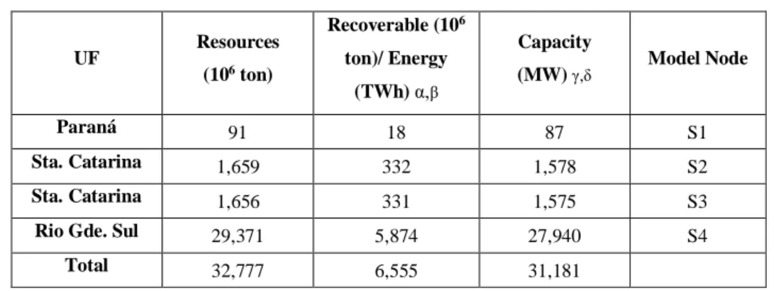
Table 1 - National coal resources, potential capacity and energy generation
UF Resources (106 ton) Recoverable (106 ton)/ Energy (TWh) α,β Capacity (MW) γ,δ Model Node Paraná 91 18 87 S1 Sta. Catarina 1,659 332 1,578 S2 Sta. Catarina 1,656 331 1,575 S3
Rio Gde. Sul 29,371 5,874 27,940 S4
Total 32,777 6,555 31,181
α URR: 28% (proven reserves - most likely), Avg mine recovery: 70% β Plant average consumption: 1000 kg/MWh
γ Avg capacity factor: 60% δ Lifetime: 40 years
Source: Own development based on [38,42]
Electricity generation potential from sugarcane biomass and other biomass crops such as soybeans and corn were taken from [38]. Other biofuel supplies are first and second generation ethanol production from sugarcane and biodiesel production from oil seeds in accordance with [30]. Finally, a number of assumptions and sources are adopted to derive RES potentials in TIMES-Brazil for wind, solar, waves and hydro, as in Table 2. Geographical locations for new hydro, sun and wind projects were taken from potential projects that already had the required documentation to participate at national auctions or a licence to build in 2015 [40].
Table 2 – Considered hydro, wind, solar and wave maximum expansion potential for the period 2020-2050 Region/Cap
(MW) Wind Hydro PV CG PV DG Waves ECSP WO ECSP WS CSP BIO
CO1 576 260 703 3,327 1,945 CO2 810 1,102 599 CO3 2,794 80 50 4,734 2,998 CO4 2,191 71 55 CO5 221 41 90 10,329 7,639 N1 11,377 235 N2 7,654 113 1,511 N3 3,303 353 N4 1,414 1,055 59 44 11 N5 2,320 252 98 462 294 N6 16,370 155 NE1 7,219 3,000 8,041 104 11,318 9,362 1,940 NE2 10,667 600 3,114 111 1,969 1,249 1,320 NE3 980 409 240 378 835 110 NE4 7,918 3,855 325 934 NE5 13,345 4,626 690 1,438 1,810 1,505 420 NE6 5,010 75 690 686 1,657 S1 9,058 391 S2 2,043 - 1,049 151 S3 325 1,413 199 1,090 S4 395 1 166 18
Region/Cap
(MW) Wind Hydro PV CG PV DG Waves ECSP WO ECSP WS CSP BIO
S5 3,644 1,200 543 1,280 S6 2,872 1 75 SE1 1 36 210 1,250 SE2 836 1,028 896 725 SE3 5,498 325 594 SE4 - 145 3,885 960 SE5 16 2,874 669 608 214 SE6 125 1,469 980 TOTAL 55,255 71490 27,481 15,566 11,430 34,674 25,217 3,790
Therefore, the centralized PV (PV-CG) potential considered by this study may be conservative. According to [45], the PV-CG potential in Brazil is around 360 GWp. For solar distributed
plants (PV-DG), we considered the generation potential in high income households in the
residential sector taken from [46,47]. This approach is also conservative as considering other income groups the capacity potential would achieve 40 GW [46,47].
Ultimately, the Brazilian gross wind potential is 7.3 TW, from which around 10% would technically suitable for generation according to [48]. CSP and waves capacity potential have been defined also by 10% reduction factor from technical potentials. Conventional CSP with and without storage (respectively ECSP WS and ECSP WO) has been taken from [49]. Hybrid CSP-biomass potential (CSP-BIO) was taken from [50]. Finally, wave potential has been defined for 11 shore-regions, taken from [51].
2.2.4 Considered variability of RES for power production
The hydro seasonal generation potential has been quantified based on yearly average inflows from the period 1931- 2015 [52] in combination with a hill chart for each of the 28 typical plants, representing the hydraulic production equation, which considers volume (hm3) and outflow
(m3/s). It also considers the turbine and generator efficiency of the specific plant [53].
Biomass availability factors from sugarcane bagasse have been set in accordance to the crop
calendar. There are two main crop periods in Brazil. The first one in the northeast (NE) region starts in September and goes through May. The second one in the southeast (SE) region is from April to January. All other biomass crops have been modelled using a yearly single value. The model considers country-specific wind and solar availability profiles for an average year for each of the 96 modelled time-slices6 from [54,55], which were created from weather station of the National Institute of Meteorology (INMET). PV resource availability has been quantified through the System Advisor Model (SAM) considering 40 solar spots. Wind resource has been
quantified from 24 wind hotspots. Every wind or PV plant uses the closest resource spot, defined at a geographic information system tool.
CSP and Waves availability factors have been modelled in a simpler manner using an annual
availability factor. The CSP availability factor varies for the different considered technologies [49]. Without-storage parabolic projects (ECSP-WO) are modelled with 11 different values spread through the same number of regions. Similarly, the with-storage CSP (ECSP-WS) has been quantified with 9 availability values. A single resource factor has been applied for wave energy for all the regional potential presented, as well as for Hybrid CSP-biomass (CSP-BIO).
2.2.5 Transmission Network (electricity exchange between regions)
The Brazilian transmission system has 130 thousand kilometres and connects almost the entire country but some isolated parts in the N macro-region. The National Interconnected System has been modelled through 59 exchange processes (lines) which connect the 29 region-nodes shown in Figure 3. Transmission flow maximum capacities are in line with official data from the national operator [56], assumed to be directly proportional to its operational voltage and current. Firstly, only 500 kV lines were selected from the real network, enabling the definition of main exchange corridors which in turn made the modelled network simpler. Then, other voltage-type lines were aggregated with those ones. It would be possible to describe network branches even in more detail, for instance as presented in a short-term operation assessment made by [55], but computational burdens would be enormous.
Imports/exports to other Latin America countries are also considered. The Brazilian energy system is operated centrally by the national TSO, which means it does not account (in principle) for an energy balance in other countries. This is different from an operation from a regional perspective, as observed in Europe (ENTSO-E), for instance. In the case of Brazil, energy imports/exports only happen when one of the neighboring countries involved asks for energy support from the other side of the line. An exception to this is “Itaipu Binacional” hydroelectric power plant, for which there is a steady import of electricity to Brazil from almost all power generation derived from the Paraguayan portion of the plant. For all cases, there is no monetary transaction, but an energy balance in the end of the period. We represented interconnections by setting a relatively high import price ($300/MWh) to force the model to operate by their own means and a lower export price ($50/MWh) to enable it to drain energy in moments of energy excess, both bounded by current existent capacity in the transmission lines. Expansion is not allowed.
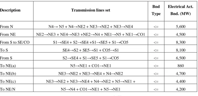
There are also transmission constraints from the Brazilian network due to electrical network procedures, which were added to the modelled network for exchanges between the Brazilian macro-regions [57], in Table 3. For example, there is a constraint for the energy coming from the
south, in which the sum of trades in parallel ‘from S2 to SE4’; ‘from S1 to SE5’ and ‘from S1 to CO5’ must not surpass 6500 MW at any given time-slice.
Table 3 - Energy flow constraints at regional exchange processes
Description Transmission lines set Bnd
Type
Electrical Act. Bnd. (MW)
From N N4→ N5 + N4→NE2 + NE3→NE2 + NE3→NE4 <= 5,600
From NE NE2→NE3 + NE4→NE3 +NE2→N4 + NE1→N5 + NE1→CO1 <= 4,500
From S to SE/CO S1→SE4 + S2→SE4 +S1→SE5 + S1→CO5 <= 8,300
To S SE4→S2 + SE5→S1 + CO5→S1 <= 8,100
From S S2→SE4 + S1→SE5 + S1→CO5 <= 6,500
To NE(a) N5→NE1 + CO1→NE1 <= 860
To NE(b) NE3→NE2 + NE3→NE4 + N4→NE2 <= 4,700
To NE(c) NE3→NE2 + NE3→NE4 + N4→NE2 + N5→NE1 + CO1→NE1
<= 4,400
To NE/N N5→N4 + CO1→NE1 + N5→NE1 <= 4,200
Source: Authors based on [57]
The grid can be expanded only by AC transmission lines (see Annex 3 for costs). Because our TIMES model treats transmission exchanges by means of a transportation model, the model cannot distinguish/choose between benefits/disadvantages in AC and DC technologies and respective related costs. Therefore, we can say that considering only AC lines is a conservative approach in terms of technical concerns, as DC lines are asynchronous and, therefore, do not contribute to the stability of the system.
The development schedule of new transmission lines is not expected to have relevant modifications until 2020. Theoretically, there would be no upper limits for new lines as grid expansion does not rely on fuel supply or natural resource availability. On the other hand, there are environmental concerns that affect expansion of current grid infrastructure. Hence, we assumed that any of the current transmission lines may expand their capacity up to 50% of installed capacity in 2020. Such assumption was tested in a sensitivity analysis described in section 3.5.
2.3 Modelled scenarios
The main goal of this paper is to evaluate to what extent it might be desirable to detail modelling transmission of electricity in terms of process exchange to assess impact in PV and wind deployment. Therefore, three different scenarios have been tested, as follows:
1. The Free Trade scenario (FT) does not consider electricity transmission. This means that generated energy at a given region could be used wherever it is needed. There are thus no
transmissions flow bottlenecks and the entire country is modelled as one single node. In short, the transmission processes do not constrain model results;
2. The Simple Trade scenario (ST) considers transmission capacities only between the five Brazilian macro-regions, i.e. the blue lines in Figure 3. Transmission attributes are considered for these inter-macro-regional exchanges, but transmission within each sub-region is not accounted for. Thus, available energy in the north macro-sub-region cannot be consumed in the southeast macro-region without going through the considered transmission processes. In other words, in this scenario transmission processes partially constrain model results;
3. The Detailed Trade scenario (DT) considers the entire transmission network within the 29 regions, i.e. both the blue and red lines in Figure 3. Therefore, any electricity exchange between regions is restrained by modelled transmission technical aspects.
Except if otherwise mentioned, all scenarios have in common the following assumptions: i) No consideration of the specific policy incentives to RES (e.g. feed-in tariffs, green certificates) since the objective is to assess deployment based solely on cost-effectiveness; ii) no environmental (e.g. GHG emissions) constraints; iii) current and planned transmission network until 2020.
Figure 3 -Spatial coverage of the TIMES_Brazil model and its disaggregation into 5 macro-regions and 29 sub-regions. All transmission lines are considered in the DT scenario, but only blue ones are considered in the ST. FTIn the map the green area corresponds to the North region (N), purple corresponds to the Northeast region (NE), the brown area is the Centre-West (CO) and Southeast (SE) regions and yellow is the South (S) region. Energy exchanges with Argentina, Paraguay (UHE Itaipu), Uruguay and Venezuela are also considered.
3 Results and discussion
3.1 Total installed capacity in 2030, 2040 and 2050
3.1.1 Total installed capacity
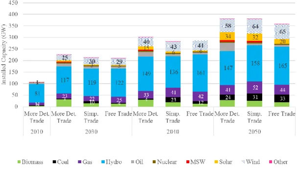
The evolution of installed capacity for the power sector is different across scenarios, but the Free and ST scenarios have closer development pathways than the DT (see Figure 4). The installed capacity increases in all scenarios from 111 GW in the base-year to 360-380 GW in 2050. The lowest total value in 2050 is for the FT Scenario, due to almost no energy loss because of no electricity transmission constraints. Therefore, in this scenario the optimisation can freely choose between cheaper generation technologies and operate more closely to a merit-order ranking. The more transmission-constrained a given scenario is, the more certain power technologies tend to come up into the system (namely solar, natural gas and heavy fuel oil). The ST scenario is somehow an intermediate level among what happens in the FT and DT scenarios. This suggests the existence of important transmission bottlenecks at a macro-regional level, as well as inter-regional’s and the importance of modelling it.
Figure 4 – Installed electricity generation capacity in GW for the three modelled scenarios
In the past years, hydro, wind and some biomass projects have achieved lowest energy prices at Brazilian auctions. A similar development pattern has been observed in the model (Figure 4). Differences in scenarios regarding hydropower development are mostly perceived in the north of Brazil, where most of the remaining potential is located (see section 2.2.3). Hydro power plants are amongst the cheapest expansion options in the Brazilian system7, therefore whenever it is possible they are selected by the model. For instance, we found a hydro capacity of 143 GW in our more transmission-constrained scenario, which is higher than the one found by [29]. In their study, the expansion of hydropower plants was capped at 3.3 GW, which is exogenously added to 109 GW of existent and planned projects. Their study also found at least around 60 GW (PV) and 80 GW (Wind) in all scenarios due to their goal of testing a 100% renewable power system for Brazil. Our results, in turn, indicated a maximum of 34 GW (PV) and 64 (Wind). The much higher renewables potential considered in their study may have also contributed to the discrepancy between both assessments.
Levelised cost of electricity (LCOE) for plants installed in the period 2020-2050 in our model are presented in Annex B.
3.2 Generated electricity in 2030, 2040 and 2050
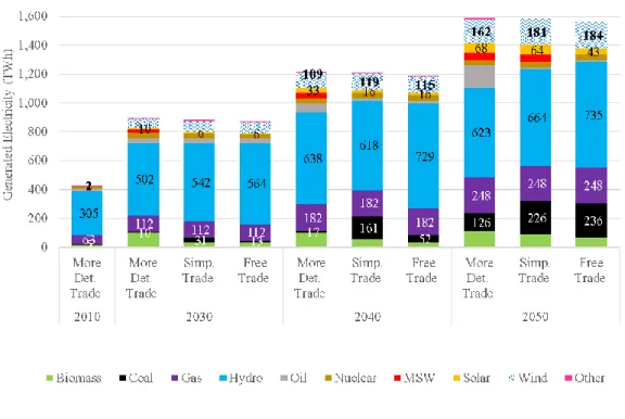
The generation profile of the power plants varies across scenario, region, year and technology itself (see Figure 5).
Figure 5 – Generated electricity in TWh for the three modelled scenarios
Most power plants in TIMES-Brazil have variable costs directly related to their production output except for wind and solar PV. This means there is no additional (activity) cost for the marginal unit of electricity generated from wind. Since the TIMES objective function is to lower total system costs, the model always deploys first the most cost-effective options in each time-slice. Thus, solar and wind are the first technologies brought on-line in the system, because although they do not have the lowest levelized cost of electricity (LCOE), they have low marginal prices. As such, solar and wind have their CF quite close to their maximum possible availability factors. Hydro power plants, which often have the next lower activity cost, come right after and so on. However, due to transmission capacity boundaries, any given power plant will only operate whether the generated energy can be consumed: i) within the region where the power plant is located, or ii) sent abroad. Therefore, not considering transmission constraints (as in the FT scenario) leads to a unit commitment schedule closely related to the system merit-order ranking. By the same rationale, taking transmission into account result in a non-optimal merit order dispatch and new units may need to be brought into operation, which otherwise would not be necessary, increasing system balancing costs 8. Furthermore, generation below optimal level increases electricity costs from a given unit, as fixed costs are shared by less generated energy.
8 Minimum levels of power operation were not declared in the presented model, although its declaration is
possible in TIMES. We opted not to include these constraints as it would increase the computational complexity. Similarly, there are no ramp up/down operation constraints declared in the model.
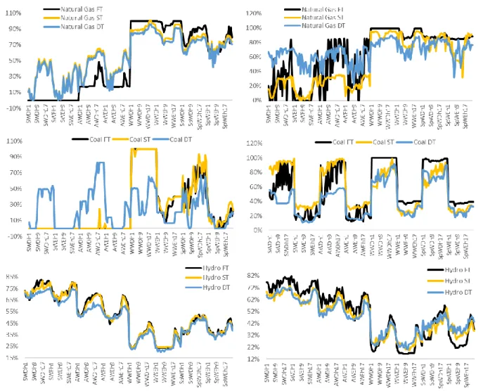
Our results show that transmission constraints impact mostly dispatchable thermal plants with medium-level marginal prices. In the FT scenario in 2030, coal, natural gas and fuel oil power plants remain off-line all summer (Figure 6). Their output is not needed due to the hydropower activity, which in FT can be freely delivered to the five macro-regions of the country. The dry period occurs with winter, reducing hydro generation and increasing the need for other sources, and thus coal and natural gas operate at full potential in Winter weekdays.
The ST scenario has installed natural gas in north macro-region, where natural gas commodity is cheaper. From there, it sends electricity to SE via the long transmission line that departs from N2 node. In the DT scenario, the same natural gas capacity is located directly in the southeast, as by doing so the model overcomes the southern inner congestion infrastructure. Hydro profiles are similar in the three scenarios, but transmission has undermined some hydro generation from north in the DT scenario.
Coal power plants become more important in the last 10-15 year in all scenarios, but at different sites. Its main role is supplying southern regions as hydro from the north encountered grid bottlenecks. However, in DT, coal which is located in the south cannot achieve the southeast due to inner bottlenecks. Due to that reason, coal capacity factor in the DT is 60%, 20 percentage points below the CF in the other two scenarios. Hydropower plants in the DT scenario operate with around 8%-10% lower CF than in FT and 3% above the hydro in the ST, although there is less hydro capacity in this scenario.
Figure 6 - Capacity factor (%) for technology groups for i) 2030 (left) and ii) 2050 (right). Time slices are coded as follows: Weekdays (xWD) and weekends (xWE) in Summer(S), Autumn(A), Winter(W) and Spring(Sp). Data for the 24 hours of all typical days.
The CF of wind and solar plants have a low variation between scenarios due to the merit-order dispatch, being must-run units. The real impact from transmission modelling over wind and solar project are only on development of new plants.
3.3 Transmission Expansion
Since the FT scenario does not consider electricity transmission processes, this section only refers to results from the ST and DT scenarios. As transmission costs are directly related to line lengths, when possible the model opts by the lowest distance between regions (or nodes). In general, transmission expansion is led by the trade-off between expanding the system by cheaper lines or doing it by longest and more expensive ones, usually to avoid grid bottlenecks in between – for instance to achieve highest demand load spots in constrained areas. Besides, inner regions constraints also influence inter-regional expansion. In the end of the period, the sum of all macro-regional bonds achieves higher capacities in the simpler scenario (Figure 7). Furthermore, some inter-regional exchange/expansions are indirectly linked to inner-regional exchange/expansion
and, therefore, the expansion of one might be required to the expansion of the other and vice-versa.
Figure 7 - Aggregated regional expansion for periods 2020-2030 (a) and 2030-2050 (b) in the ST and DT scenarios
As a matter of comparison, the good exercise made by [29] found a 54-59 GW expansion by 2050 depending on their scenarios. Our results indicated an expansion of 38-46 GW in our sensitive scenarios (please see section 3.5), but less so in the others. We added upper expansion boundaries though, which were achieved at some power transmission lines. In that sense, we found significant expansion between the north and south/southeast regions, contrarily to results from [29], probably because they had extremely low hydro expansion in their results and the remaining hydro potential in Brazil is mostly located in the north of the country
3.4 Regional electricity price variation vis-à-vis the ones of the year 2030 and 2050
Prices for delivering an additional power unit at a given time-slice period are a function of the cost of producing and transmitting electricity from the different sources that make up the electricity pool, weighed by an electricity availability level in that time-slice as result of the balance between supply and demand. At moments in which supply equals demand, marginal energy prices may be understood as the electricity shadow price, which describes the cost change in the objective function as a consequence of an increase of electricity demand by one unit. Prices may also achieve lower values or even zero, meaning an over production of the commodity due to imposed constraints in the model [58]. There are two components that may impact electricity marginal prices at a given region: local power prices and the exchange power price. The former
is set by the most expensive power source under operation in the region. The latter is .weighed by neighbour prices, when imports are applied9.
The merit-order ranking defines the marginal plant able to produce an additional unit of energy at the lowest cost available. Although similar, the merit-order is not set by levelized costs of energy, rather by plants variable costs. Plants under operation with lower costs than the one set in the market earn an economic rent for the electricity generated. Therefore, their profit is the difference between the current price and their own short-run marginal cost.
The current model has two different electricity commodities. The combination between marginal prices from local electricity and exchange prices for the imported electricity results in a high-voltage marginal price. There is also a distribution process within every region which produces a low-voltage electricity commodity. Since there is electricity loss in every distribution process, the low-voltage electricity is always more expensive than high-voltage and is the one later supplied to final consumers. Average low-voltage marginal prices for the modelled scenarios are presented in Table 4 and figures 8-11.
Table 4 - Seasonal electricity prices for each scenario
Summer Fall Winter Spring
FT Electricity Marginal Price (US$/MWh) 2030 28 65 129 67 2040 74 74 112 103 2050 125 125 179 125 ST 2030 47 90 126 105 2040 90 106 136 106 2050 140 183 200 189 DT 2030 48 113 165 144 2040 93 173 199 176 2050 213 271 303 277
Electricity prices in Brazil present a correlation with water availability at hydrological basins, which have larger water inflows from December until May, so this is the period in which prices are expected to reach lower values. Beyond water variability, results show transmission network as having a relevant impact on power prices. On average, the ST scenario is around 25% more expensive than FT, while DT is 77% more expensive than FT.
Due to lack of boundaries, trade costs and other constraints, there is no price variability in the FT scenario in any time-slice and year (Figure 8). It may be perceived as an average of the entire system. As expected, the ST scenario has prices variability mainly between macro-regions. DT scenario is more expensive on the average, but has cheaper prices than the ST scenario in the mid-west, where around 80% of total energy is from hydro units. However, only part of this cheap
power can achieve the southeast region, which instead must produce locally. Hence, the more transmission-constrained a scenario is, the more is the electricity produced locally.
Figure 8 - Electricity prices in summer in 2030, for FT (upper-left), ST (upper-right) and DT (lower-center) scenarios.
The dry season in the winter has higher power prices mostly everywhere, as the low levels of hydro generation are replaced by more expensive sources (Figure 9). The variability gap between rainy and dry periods is worse in the north, where large run-of-river hydropower plants are located. The exception in the dry season is in hydro units from the lower south, which present a good generation profile in the period. However, this energy is not sent to the southeast in DT, as it is in ST, because of inner bottlenecks. Thus, southern marginal prices in the detailed scenario are quite cheaper compared to the ST scenario.
Figure 9 - Electricity prices in winter in 2030, for FT (upper-left), ST (upper-right) and DT (lower-center) scenarios
In 2050, the big picture for the entire country shows a free and simple scenario mostly supported by hydro and coal units, as in detailed scenario coal units are replaced by natural gas and fuel oil, pushing prices do the edge. While there is no generation from these sources in summer for free scenario, natural gas is responsible for 54 TWh and 21 TWh, respectively, in detailed and simple scenario as well as fuel oil accounts for 19 TWh and 2 TWh.
Figure 10 - Electricity prices in the summer in 2050, for FT (upper-left), ST (upper-right) and DT (lower-center) scenarios
As in 2030, prices in the middle of the year are higher due to the lower water availability. Assessing the Brazilian energy system in winter is important, as it enables evaluating the capacity of the country to provide energy with lower contribution from hydropower. The winter energy profile (TWh) in 2050, respectively for free, simple and detailed scenario are: hydro (102 /100/ 99); natural gas (94/102/72), coal (71/51/38), fuel oil (9/6/52), biomass (30/36/41), wind (55/54/47), PV (7/9/8), CSP (8/8/11), USW (0/13/13) and nuclear (9/9/9).
Figure 11 - Electricity prices in winter in 2050, for FT (upper-left), ST (upper-right) and DT (lower-center) scenarios
3.5 Sensitivity Analysis to assumptions on transmission grid expansion
Two sensitive scenarios have been applied on the DT only, i.e., the more transmission-constrained scenario. The main objective was to test variations in the upper expansion boundary set in section 2.2.5, as this value is not based on a well-defined boundary, as it was made, for instance, in the case of solar, wind or hydro potentials.
The first scenario assessed a 100% expansion at transmission lines (DT 100%), rather than 50% as previously. The second (DT 100% - WoEr) has not considered the electrical boundaries presented in Table 3. *Transmission was gathered by different sets in regard to the type of exchange, which may be inter-regional or inter sub-regional. For instance, the set CO/SE-S stands for all exchange processes between mid-west (CO)/southeast (SE) and south (S) regions and ‘Inner NE’ stands for all transmission lines within northeast (NEx).
Figure 12 shows the ration between installed capacity between regular and sensitive scenarios, in which values above the unity mean the sensitive scenario capacity surpasses the one from regular detailed. In the “DT 100% - WoEr” case, inner south transmission lines capacity exceeds in more
than 60% the capacity from the regular 50%-detailed scenario. This deviation was somehow expected as it stresses transmission bottlenecks already mentioned at different parts of this work.
*Transmission was gathered by different sets in regard to the type of exchange, which may be inter-regional or inter sub-regional. For instance, the set CO/SE-S stands for all exchange processes between mid-west (CO)/southeast (SE) and south (S) regions and ‘Inner NE’ stands for all transmission lines within northeast (NEx).
Figure 12 - Transmission capacity deviation in relation to detailed-50% for detailed-100% and detailed-100% without electrical boundaries
The “DT 100%” case increased very little coal, wind and PV, and decreased biomass and fuel oil also slighly (Figure 13). But in general, there is no relevant modification in technologies installed capacities. The scenario without electrical constraints in turn presented a strong growth in coal and wind in 2030 and in hydropower and PV capacity, as well as an important decrease in fuel oil use, which is partially due to a higher transmission capacity between the north (high hydro potential) and the southeast (high demand load) regions. It is worth to mention that a capacity decrease in PV in 2030 followed by an increase in 2050, which means that the technology is not economic viable in the medium term based on its costs. Similarly, a strong growth in coal took place in 2030, highlighting the low costs of this technology.
0.50 1.00 1.50
CO/SE - N CO/SE - NE CO/SE - S Inner CO/SE
Inner N Inner NE Inner S N - NE Det 100%/Det 50% Det 100% (WoEr)/Det 50%
Figure 13 - Capacity variation between regular detailed scenario, 100% detailed and 100% WoEr
4 Final Remarks and Conclusions
This study attempted to stress the importance of better modelling transmission constraints in a long-term energy system optimization model. This is particularly relevant in large, and climate-diverse, countries, such as Brazil, planning to install RES. Modelling transmission in detail helps to understand:
- How the existence of inner sub-regional constraints can impact inter-regional expansion, so one may be required for the development of the other.
- How the power plant expansion fleet may differ significantly as transmission modeling increases. Our results also show that transmission constraints impacted mostly dispatchable thermal plants, which have medium-level marginal prices. Coal becomes important with the lack of hydro, but bottlenecks can also improve the economics of natural gas over coal.
- That less constraints scenarios enables accessing the best available resources, either the best solar/wind spots to generate energy or lowest fossil fuel prices spots. Therefore, they may provide an optimistic view of RES expansion without costs to debottlenecking transmission constraints.
- That transmission bottlenecks do not impact so much wind and solar generation profiles (capacity factors), rather it impacts the development of new projects. Projects are only
4.0 0.20 0.40 0.60 0.80 1.00 1.20 1.40 1.60 1.80 2.00 Biomass Natural Gas
Coal CSP Fuel Nuclear Wind Hydro Others PV
C ap aci ty var iat io n 2028 DT 2028 DT 100% 2028 DT 100% (WoEr) 2048 DT 2048 DT 100% 2048 DT 100% (WoEr)
placed where the likelihood to deliver the generation is high and may occur even in poor wind-resource sites if there is need for new generation locally produced
- That more transmission-constrained scenarios tend to produce more energy closer to the main demand loads.
- Electricity marginal prices could decrease up to zero at times of electricity over production at a node due to either renewable availability higher than demand or transmission bottlenecks.
- The more transmission constrained a scenario is, the more expensive it will be. In our Brazilian study, on average, the ST scenario is around 25% more expensive than FT, while DT is 77% more expensive than FT.
These findings are relevant for energy and climate policy support. Frequently energy system models as TIMES, MESSAGE or PRIMES are used to develop medium to long-term RES and GHG emission abatement targets. By highlighting the effect that transmission bottlenecks can have in RES deployment we hope to provide more robust information to policy makers. Another policy relevant finding might be the differences in prices at different nodes, when considering detailed grid processes. This could be important to consider when looking into electricity pricing models for such a large country as Brazil. To what extent should citizens living in different parts of the country pay a cheaper/more expensive electricity price? And how could such price differences then be dealt with?
Regarding limitations of this study, it should be noted that solar and wind availability factors were quantified hourly, then aggregated to the time-slice level using average values for each time-slice period. Going that way loses some variability patterns in the natural resource. To overcome this limitation, some authors suggested the use of representative days [59], which may be applied on further work. Besides, no modelling scenarios could detect eventual capacity factor decrease at wind and solar units. Hence, further flexibility attributes such as ramp up/downs, minimal operation power levels and others should be needed.
Acknowledgements
We thank the Brazilian Federal agencies CAPES (Coordenação de Aperfeiçoamento de Pessoal de Nível Superior) and CNPq (Conselho Nacional de Desenvolvimento Científico e Tecnológico) for their support for the scientific research performed at the Energy Planning Program, Universidade Federal do Rio de Janeiro. We would also like to thank the European Commission for their support to the scientific research performed jointly by the Energy Planning Program and the Center for Environmental and Sustainability Research.
ANNEX
Annex A – Characteristics of considered power plants that can be deployed between 2020 and 2050 Technology Investment Costs ($/kW) (2020-2050) Fixed Costs ($/kW) Variable Costs ($/MWh) (2020-2050) Fuel Costs ($/MWh) Maximum possible Capacity factor Efficiency (%) COAL Coal-Fluidized Bed Combustion (FBC) 1700 - 1500 39 4.6-3.0 40 0.85 38%-42% Coal-FBC + Biomass (Cofiring) 3690 39 4.1-2.5 40/ 0.7/0.3 35%-40% Coal-Pulverized Combustion (PC) 2200 38 5.6-5.4 90 0.85 40%-45% Coal - IGCC 2400 68 3.6-3.4 90 0.85 40%-48% NATURAL GAS
Open Cycle Gas
Turbine (OCGT) 800-600 20 4.0-3.2 27-35/24 (N) 0.6 35%-.38%
Combined Cycle Gas
Turbine (CCGT) 1190-1000 18 6.0-4.6 27-35/24 0.85 50%-55%
OIL
Heavy Fuel Oil
(HFO) 1000 125 48 0.55 30%
Light Fuel Oil (LFO) 1070 125 64-95 0.35 30%
HYDRO
Hydro small 2,936 65 3.0-1.8 Seasonal/Geogr
aphical
Hydro medium 2513 58 2.6-1,8 Seasonal
Hydro High 2091 52 3.8-2.4 Seasonal
NUCLEAR
Nuclear 4000 136 0.8-0.6 9 0.9 33%
BIOMASS
Biomass (Residues) 3600 10 5.5-5.2 58 0.50 28%
Biomass (Sugarcane) 350 17.5 4.7-4.6 250-450 Seasonal Municipal Solid
Waste (MSW) 7050-6210
250-200 0.74
OTHERS RES
PV Plant size (CG) 4300-1000 45-30 Hourly-seasonal
Technology Investment Costs ($/kW) (2020-2050) Fixed Costs ($/kW) Variable Costs ($/MWh) (2020-2050) Fuel Costs ($/MWh) Maximum possible Capacity factor Efficiency (%) Concentrated Solar Power (CSP) 7000-6500 70 2.6-1.9 0.20 CSP with 4h storage 5200-3500 90 2.8-2.2 0.31 CSP with 6h storage 6200-4100 125 2.8-2.2 0,42 CSP with 12h storage 7200-4600 160 2.8-2.2 0.44 CSP-BIO 5800-3900 145 2.8-2.2 -/58 0.51 -/28%
Wind Onshore 1810-1550 38 Hourly-seasonal
Wind-Off Shore 5000-3500 65-58 0.4
Wave 6000-4500 20 0.15
. Source: [60–62]
Annex B – Levelized Costs of Electricity obtained using TIMES_Brazil in $/MWh for new installed capacity Technology 2020-2030 2030-2040 2040-2050 2020-2030 2030-2040 2040-2050 2020-2030 2030-2040 2040-2050
Scenario FT scenario ST Scenario DT Scenario
Thermal units fuelled by domestic coal 97.2 91.2 – 94.1 89.5 – 90.7 93.1 – 93.3 89.6 87.9 93.1 90.1 Thermal units fuelled by Imported Coal 262.4 – 265.0 250.3 – 263.1 Natural Gas CCGT (NG) 62 100 128 31.4 28.2 - 86.2 26.7 - 92.3 35.6 – 91.8 32.8 – 101.8 85.5 Hydro 69.46 - 85.9 78.08 - 94.56 95.35 - 114.14 55.2 - 118.6 55.6-139.0 58.0 – 164.1 64.3 – 222.3 70.8 – 243.7 109.0 – 307.7 Biomass 136.23 156.2 136.2 – 176.0 136.3 – 195.7 Sugarcane Biom. 38.7-43.4 46.0-47.5 138.9 – 151.1 474.2 Nuclear 71.4 71.29 74.2
Heavy Fuel Oil
(HFO) 96 106-121 171 111.7 146.1 -147.7 185.0 – 220.4 238.6 – 243.8 236.2
Light Fuel Oil (LFO) 90.4 - 90.5 130.8 – 148.6 296.7 – 318.0 Municipal Solid Waste (MSW) 126.42 130.9 126.4 126.4 Wind 78.0 – 84.3 89.5-97.1 111.6-120.1 75.2 – 119.8 80.7 – 148.3 88.0 – 194.3 62.2 – 201.3 59.9 – 266.5 58.4 – 342.7 PV CG 120.0-121.5 94.3 – 218.7 229.3 – 266.5 93.7 – 342.7 Concentrated Solar Power (CSP) 118 135 75.7 114.9 163.3 – 198.9 122.5 – 190.8 136.4 – 264.8 148.0 – 371.6 H2 218.7 218.7. 218.7
Annex C – Transmission Costs (Alternating Current) Technology Station Costs
(million $/line) Line Costs ($/kW) O&M Costs ($/km-year) Variable Costs ($/MWh) AC Lines 70 1500 40 0.45 Source: [12]
5 References
[1] OECD/IEA, Renewable Energy Medium-Term Market Report 2016., Organisation for Economic Cooperation and Development / International Energy Agency, Paris, 2016. http://www.iea.org/publications/freepublications/publication/MTRMR2016.pdf.
[2] OECD/IEA, Energy Technology Perspectives 2017., Organisation for Economic Cooperation and Development / International Energy Agency, Paris, 2017.
[3] J. Widén, N. Carpman, V. Castellucci, D. Lingfors, J. Olauson, F. Remouit, M. Bergkvist, M. Grabbe, R. Waters, Variability assessment and forecasting of renewables: A review for solar, wind, wave and tidal resources, Renewable and Sustainable Energy Reviews. 44 (2015) 356–375. doi:10.1016/j.rser.2014.12.019.
[4] K. Suomalainen, C. Silva, P. Ferrão, S. Connors, Wind power design in isolated energy systems: Impacts of daily wind patterns, Applied Energy. 101 (2013) 533–540. doi:10.1016/j.apenergy.2012.06.027.
[5] Y. Rombauts, E. Delarue, W. D’haeseleer, Optimal portfolio-theory-based allocation of wind power: Taking into account cross-border transmission-capacity constraints, Renewable Energy. 36 (2011) 2374–2387. doi:10.1016/j.renene.2011.02.010.
[6] R. Komiyama, Y. Fujii, Assessment of massive integration of photovoltaic system considering rechargeable battery in Japan with high time-resolution optimal power generation mix model, Energy Policy. 66 (2014) 73–89. doi:10.1016/j.enpol.2013.11.022. [7] J. Schmidt, G. Lehecka, V. Gass, E. Schmid, Where the wind blows: Assessing the effect
of fixed and premium based feed-in tariffs on the spatial diversification of wind turbines, Energy Economics. 40 (2013) 269–276. doi:10.1016/j.eneco.2013.07.004.
[8] S. Collins, J.P. Deane, B. Ó Gallachóir, Adding value to EU energy policy analysis using a multi-model approach with an EU-28 electricity dispatch model, Energy. 130 (2017) 433– 447. doi:10.1016/j.energy.2017.05.010.
[9] S. Collins, J.P. Deane, K. Poncelet, E. Panos, R.C. Pietzcker, E. Delarue, B.P. Ó Gallachóir, Integrating short term variations of the power system into integrated energy system models: A methodological review, Renewable and Sustainable Energy Reviews. 76 (2017) 839–856. doi:10.1016/j.rser.2017.03.090.
[10] M. Zeyringer, H. Daly, F. Birgit, E. Sharp, N. Strachan, Spatially and temporally explicit energy system modelling to support the transition to a low carbon energy infrastructure- Case study for wind energy in the UK., in: ISNGI 2014, London, UK., 2015: p. 7.
[11] IRENA, Planning for the renewable future - Long-term modelling and tools to expand variable renewable power in emerging economies., International Renewable Energy Agency, Abu Dhabi, 2017.
[12] IEA, The Power of Transformation - Wind, Sun and the Economics of Flexible Power Systems, International Energy Agency, Paris, 2014.
[13] L. Hirth, F. Ueckerdt, O. Edenhofer, Why Wind is Not Coal: On the Economics of Electricity, Social Science Research Network, Rochester, NY, 2014. http://papers.ssrn.com/abstract=2428788 (accessed September 19, 2016).
[14] ONS, Histórico Da Operação – Série Capacidade Instalada, Operador Nacional do Sistema Elétrico., Rio de Janeiro, 2018.
[15] S. Simoes, W. Nijs, P. Ruiz, A. Sgobbi, C. Thiel, Comparing policy routes for low-carbon power technology deployment in EU – an energy system analysis, Energy Policy. 101 (2017) 353–365. doi:10.1016/j.enpol.2016.10.006.
[16] A.F.P. Lucena, L. Clarke, R. Schaeffer, A. Szklo, P.R.R. Rochedo, L.P.P. Nogueira, K. Daenzer, A. Gurgel, A. Kitous, T. Kober, Climate policy scenarios in Brazil: A multi-model comparison for energy, Energy Economics. 56 (2016) 564–574. doi:10.1016/j.eneco.2015.02.005.
[17] L.P.P. Nogueira, A. Frossard Pereira de Lucena, R. Rathmann, P. Rua Rodriguez Rochedo, A. Szklo, R. Schaeffer, Will thermal power plants with CCS play a role in Brazil’s future electric power generation?, International Journal of Greenhouse Gas Control. 24 (2014) 115–123. doi:10.1016/j.ijggc.2014.03.002.
[18] P. Fragkos, N. Tasios, L. Paroussos, P. Capros, S. Tsani, Energy system impacts and policy implications of the European Intended Nationally Determined Contribution and low-carbon pathway to 2050, Energy Policy. 100 (2017) 216–226. doi:10.1016/j.enpol.2016.10.023. [19] P. Capros, L. Paroussos, P. Fragkos, S. Tsani, B. Boitier, F. Wagner, S. Busch, G. Resch,
M. Blesl, J. Bollen, Description of models and scenarios used to assess European decarbonisation pathways, Energy Strategy Reviews. 2 (2014) 220–230. doi:10.1016/j.esr.2013.12.008.
[20] S. Simoes, M. Zeyringer, D. Mayr, T. Huld, W. Nijs, J. Schmidt, Impact of different levels of geographical disaggregation of wind and PV electricity generation in large energy system models: A case study for Austria, Renewable Energy. 105 (2017) 183–198. doi:10.1016/j.renene.2016.12.020.
[21] M. Labriet, A. Kanudia, R. Loulou, Climate mitigation under an uncertain technology future: A TIAM-World analysis, Energy Economics. 34 (2012) S366–S377. doi:10.1016/j.eneco.2012.02.016.
[22] M. Haller, S. Ludig, N. Bauer, Decarbonization scenarios for the EU and MENA power system: Considering spatial distribution and short term dynamics of renewable generation, Energy Policy. 47 (2012) 282–290. doi:10.1016/j.enpol.2012.04.069.
[23] R. Soria, A.F.P. Lucena, J. Tomaschek, T. Fichter, T. Haasz, A. Szklo, R. Schaeffer, P. Rochedo, U. Fahl, J. Kern, Modelling concentrated solar power (CSP) in the Brazilian energy system: A soft-linked model coupling approach, Energy. 116 (2016) 265–280. doi:10.1016/j.energy.2016.09.080.
[24] D. Malagueta, A. Szklo, B.S.M.C. Borba, R. Soria, R. Aragão, R. Schaeffer, R. Dutra, Assessing incentive policies for integrating centralized solar power generation in the Brazilian electric power system, Energy Policy. 59 (2013) 198–212. doi:10.1016/j.enpol.2013.03.029.
[25] J.B.S.O.D. Andrade Guerra, L. Dutra, N.B.C. Schwinden, S.F. de Andrade, Future scenarios and trends in energy generation in brazil: supply and demand and mitigation forecasts, Journal of Cleaner Production. 103 (2015) 197–210. doi:10.1016/j.jclepro.2014.09.082. [26] M.J. Santos, P. Ferreira, M. Araújo, J. Portugal-Pereira, A.F.P. Lucena, R. Schaeffer,
Scenarios for the future Brazilian power sector based on a multi-criteria assessment, Journal of Cleaner Production. 167 (2017) 938–950. doi:10.1016/j.jclepro.2017.03.145.
[27] B. Soares M.C. Borba, A. Szklo, R. Schaeffer, Plug-in hybrid electric vehicles as a way to maximize the integration of variable renewable energy in power systems: The case of wind generation in northeastern Brazil, Energy. 37 (2012) 469–481. doi:10.1016/j.energy.2011.11.008.
[28] T. Fichter, R. Soria, A. Szklo, R. Schaeffer, A.F.P. Lucena, Assessing the potential role of concentrated solar power (CSP) for the northeast power system of Brazil using a detailed power system model, Energy. 121 (2017) 695–715. doi:10.1016/j.energy.2017.01.012. [29] H. Gils, S. Simon, R. Soria, H.C. Gils, S. Simon, R. Soria, 100% Renewable Energy Supply
for Brazil—The Role of Sector Coupling and Regional Development, Energies. 10 (2017) 1859. doi:10.3390/en10111859.
[30] L.P.N. Oliveira., Temporal issues in mitigation alternatives for the energy sector in Brazil, PhD Thesis, Energy Planning Program - Federal University of Rio de Janeiro, 2016. [31] EPE, Estudos da Demanda de Energia 2050 – Plano Nacional de Energia, Energy Research
Company, Rio de Janeiro, Brazil, 2016.
[32] EPE, Brazilian 2016 Statistical Yearbook of electricity - 2015 baseline year, Energy Research Company, Rio de Janeiro, Brazil, 2016.
[33] EPE, Energia Termelétrica - Gás Natural, Biomassa, Carvão, Nuclear, Empresa de Pesquisa Energética, Rio de Janeiro, 2016.
[34] EPE, Plano Nacional de Energia 2030 - Geração Termelétrica (Carvão MIneral), Empresa De Pesquisa Energética., Rio de Janeiro, 2007.
[35] R. Miranda, R. Soria, R. Schaeffer, A. Szklo, L. Saporta, Contributions to the analysis of “Integrating large scale wind power into the electricity grid in the Northeast of Brazil” [Energy 100 (2016) 401–415], Energy. 118 (2017) 1198–1209. doi:10.1016/j.energy.2016.10.138.
[36] P.R.R. Rochedo, B. Soares-Filho, R. Schaeffer, E. Viola, A. Szklo, A.F.P. Lucena, A. Koberle, J.L. Davis, R. Rajão, R. Rathmann, The threat of political bargaining to climate mitigation in Brazil, Nature Climate Change. 8 (2018) 695–698. doi:10.1038/s41558-018-0213-y.
[37] R. Loulou, G. Goldstein, A. Kanudia, A. Lehtilä, U. Remme, Documentation for the TIMES Model - Part I, Energy Technology Systems Analysis Programme, 2016.
[38] R. Loulou, A. Lehtilä, A. Kanudia, U. Remme, G. Goldstein, Documentation for the TIMES Model - Part II, Energy Technology Systems Analysis Programme, 2016.
[39] A. Pina, C. Silva, P. Ferrão, Modeling hourly electricity dynamics for policy making in long-term scenarios, Energy Policy. 39 (2011) 4692–4702. doi:10.1016/j.enpol.2011.06.062.
[40] ANEEL, Sistema de Informações Georreferenciadas do Setor Elétrico (SIGEL), Electricity Energy National Agency, Brasília, 2016.
[41] T.A. Saraiva, A. Szklo, A.F.P. Lucena, M.F. Chavez-Rodriguez, Forecasting Brazil’s crude oil production using a multi-Hubbert model variant, Fuel. 115 (2014) 24–31. doi:10.1016/j.fuel.2013.07.006.
[42] Petrobras, Gasoduto Urucu-Coari-Manaus inicia operação comercial., Petrobras Press Agency. (2009) 2.
[43] Petrobras, AM: Gás natural muda matriz energética da Região Norte., Petrobras Press Agency. (2011) 2.
[44] IBRAM, Ccx: mina de san juan terá produção de 25 milhões de toneladas por ano., Brazilian MIne Association Press. (2012).
[45] R. Schaefer et al., Potencial de Integração em Larga Escala de Energia Solar (Fotovoltaica e Térmica) para Geração Centralizada de Eletricidade no Brasil, Energy Planning Program, Graduate School of Engineering, Universidade Federal do Rio de Janeiro, Rio de Janeiro, 2012.
[46] R.F.C. Miranda, Photovoltaic solar energy distributed Generation Insertion analysis In the Brazilian residential sector, Thesis, Energy Planning Program, Graduate School of Engineering, Universidade Federal do Rio de Janeiro, 2013.
[47] R.F.C. Miranda, A. Szklo, R. Schaeffer, Technical-economic potential of PV systems on Brazilian rooftops, Renewable Energy. 75 (2015) 694–713. doi:10.1016/j.renene.2014.10.037.