STUDY OF ELASTIC PROPERTIES AS FUNCTION OF TEMPERATURE IN ANISOTROPIC CRACKED MEDIA: AN ULTRASONIC APPROACH

www.scielo.br/rbg

STUDY OF ELASTIC PROPERTIES AS FUNCTION OF TEMPERATURE

IN ANISOTROPIC CRACKED MEDIA: AN ULTRASONIC APPROACH

José Jésus Silva Sobrinho

, José J. S. de Figueiredo

, Rafael L. Lima

,

Léo Kirchhof Santos

and Murillo J. Nascimento

ABSTRACT.The study of seismic wave velocities and their related anisotropy parameters provides important tools to the study of Earth’s subsurface. The analysis of temperature’s influence in the elastic properties of synthetic rocks, e.g., may be a good alternative for modelling the response of elastic properties of rocks surrounding deep wells and/or that are submitted to the process of steam injection. In order to understand the effects of temperature on the elastic parameters, in this work we constructed four porous synthetic sandstones, one representing an uncracked medium and three cracked samples. They were submitted to variable temperatures, while their elastic properties were calculated during heating and cooling processes. It was noted that P- and S-wave velocities decreased with increasing temperature. This behavior may be caused by changes in the background stiffness and by the generation of secondary cracks inside the samples. However, P- and S- anisotropy parameters were not affected by the changes in temperature. This can be an indicative that randomly distributed secondary cracks were created. Other indicative of secondary cracking formation can be associated to the difference between seismic velocities during the heating and cooling processes.

Keywords: cracked media, anisotropy, temperature dependence, elastic parameters.

RESUMO.O estudo das ondas sísmicas e de seus parâmetros anisotrópicos associados fornece ferramentas importantes para o estudo da subsuperfície da Terra. A análise da influência da temperatura nos parâmetros elásticos de rochas sintéticas, por exemplo, pode ser uma boa alternativa para modelar a resposta das propriedades elásticas de rochas circundando poços profundos e/ou que são submetidas a processos de injeção de vapor. Para entender os efeitos da temperatura nos parâmetros elásticos, neste trabalho construímos quatro arenitos sintéticos porosos, um representando um meio não-fissurado e três amostras fissuradas. As amostras foram submetidas a temperaturas variadas, enquanto suas propriedades elásticas foram calculadas ao longo dos processos de aquecimento e resfriamento. Notou-se que as velocidades das ondas P e S diminuíram com o aumento da temperatura. Esse comportamento talvez seja causado por variações na rigidez do background e pela formação de fissuras secundárias nas amostras. Entretanto, os parâmetros anisotrópicos P e S não foram afetados pelas mudanças de temperatura. Isso pode ser considerado um indicativo de que fissuras secundárias distribuídas aleatoriamente foram formadas. Outro indicador da formação de fissuras secundárias pode ser associado à diferença entre as velocidades sísmicas durante os processos de aquecimento e resfriamento.

Palavras-chave: meios fissurados, aniostropia, dependência de temperatura, parâmetros elásticos.

1_{Universidade Federal do Pará, Faculty of Geophysics, Petrophysics and Rock Physics Laboratory - Prof. Dr. Om Prakash Verma, Belém, PA, Brazil - E-mails:} [email protected], [email protected], [email protected], [email protected], [email protected]

2_{Universidade Federal do Pará, Postgraduate Programme in Geophysics, Belém, PA, Brazil} 3_{Instituto Nacional de Ciência e Tecnologia de Geofísica do Petróleo (INCT-GP), Salvador, Brazil}

medium have been the subject of many studies along the years due to its great occurrence in sedimentary rocks and its importance to the oil industry. Thomsen (1986) has shown that, in the case of weak anisotropy (10%-20%), the anisotropy of a medium can be described using three parameters:ε,γandδ.

Investigating the temperature and pressure effects on seismic velocities of halite salt, Yan et al. (2016) concluded that the temperature effect on the velocities is dominant relative to the stress effect. Timur (1977) measured acoustic velocities in sandstone and carbonate samples as a function of temperature and found that the average decrease for a 100◦_{C rise in}

temperature was 1.7% for compressional wave velocities and 0.9% for shear wave velocities. Kern (1978) investigated the effect of high temperature and high confining pressure on compressional wave velocities in rocks of different types and found that the velocities generally decrease with temperature, but the rate varies according to the rock type. Furthermore, he concluded that, at higher isobaric pressures, the velocity drop as function of temperature decreases and the velocity-temperature relationships tend to become more and more linear functions.

Other studies have observed a decrease in elastic modulus (Zhang et al., 2009; Brotóns et al., 2013) with increasing temperature, which accounts for a decrease in seismic velocities. Thermal gradient cracking has been found to be the dominant mechanism for fracture formation in experiments conducted at low confining pressure, resulting on the decreasing of seismic wave velocities with temperature (Jansen et al., 1993). Most of the previously mentioned works did not study the anisotropy dependence on temperature. Kern & Fakhimi (1975), however, studied the influence of temperature on anisotropy in various metamorphic rocks under high pressure conditions, and observed that fabric-induced seismic anisotropy is generally unaffected by temperature. On this study, however, Kern & Fakhimi (1975) analyzed only P-wave anisotropy.

METHODOLOGY

The construction of the synthetic rock samples as well as the ultrasonic measurements were performed at the Laboratory of Petrophysics and Rock Physics – Dr. Om Prakash Verma (LPRP) at the Universidade Federal do Pará, Brazil. The following methodology description corresponds to the production of fractured or cracked synthetic sandstones.

Sample preparation

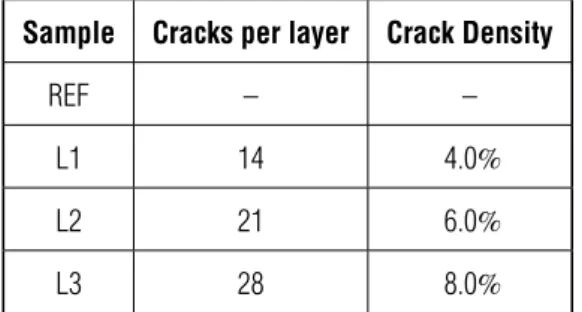
We employed the methodology developed by Santos et al. (2017) for crafting synthetic VTI samples, which is based on: cement, sand, styrofoam and paint thinner. Four samples were constructed with different crack densities. Table 1 shows the number of cracks per layer and the crack density of each sample. In order to ensure that the samples had the same composition, so that the differences in elastic properties were caused only by different crack densities, all samples were crafted simultaneously at the same mold, as can be seen in Figure 1.

Table 1 – Crack densities of the samples evaluated using Eq. 1. Sample Cracks per layer Crack Density

REF – –

L1 14 4.0%

L2 21 6.0%

L3 28 8.0%

The mortar used in the samples construction was composed of 70% sand and 30% cement. Moreover, the proportion of water was kept constant to ensure the samples homogeneity in composition. The cracks were disposed on layers constructed one

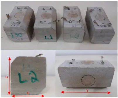
Figure 1 – Crafting process of the samples showing the styrofoam discs disposed at the top of the mortar layer and the resistances positioned inside of samples. The Figure 2 shows all samples cut and after the chemical launching to remove the styrofoam discs.

Figure 2 – Image of the four samples constructed and analyzed in this work.

at a time. At first, we filled the mold with a 2 cm layer of mortar and then placed penny-shaped styrofoam sections that were 0.5 cm in diameter and 0.1 cm thick (Fig. 1). We then filled another 0.5 cm layer of mortar and placed another set of penny-shaped cuts at the same area (4 cm x 4 cm) as before. This process was repeated until we had 7 layers with cracks spaced by 0.5 cm. Finally, we filled the last 2 cm thick layer totalizing a height of 7 cm.

Right after filling the first layer, nichrome resistance pairs were placed in the regions of each sample (Fig. 1). Those resistances are part of the temperature control system which is

described in Silva Sobrinho et al. (2017). To enable for the 45◦

measurements, the location where the resistances were placed at the mold was chosen taking into account the 45◦ _{cuts made}

afterwards on the edges of the samples. As a matter of fact, the dimensions of the samples were chosen so that a cross section of the XZ-plane would be approximately a square, which in turn would enable propagation in the 45◦_direction.

The curing time of mortars produced with cement was about eight days (Garcia et al., 2011). Once the curing time was over we had the samples sawed apart. From Santos et al. (2017), to create

where Niis the total number of penny-shaped inclusions, hiis the

aperture (thickness) of inclusion, riis the radius of the inclusion

and Vmis the model volume (only) occupied by cracks.

Ultrasonic setup and Data acquisition

The ultrasonic measurements were performed using the LPRP ultrasonic system with the same pulse transmission technique as performed in De Figueiredo et al. (2013), Santos et al. (2016) and De Figueiredo et al. (2018). The sample rate by channel for all measures of P- and S-waveforms was 0.005µs. Figure 3 shows the ultrasonic system. The system is compound by a pulser-receiver 5072PR and a preamplifier 5660B by Olympus, a 50 MHz USB oscilloscope by Handscoope, and two transducers of 1 MHz (P-wave) and 500 kHz (S-wave) by Olympus.

Figure 3 – Ultrasonic measurement system showing the pre-amplifier, the oscilloscope, the pulse-receiver and the P-and S-wave transducers.

The measurements were realized in the directions 0◦_{, 45}◦

and 90◦_{, being 90}◦ _{the direction parallel to the cracks, 0}◦

the direction perpendicular to the cracks and 45◦ _{diagonal to}

the cracks. Figure 4 depicts the directions of propagation and polarization assigned on this study. All the measurements were performed with the sample temperature varying from from 25◦_C

to 130◦_{C. Temperature step was 15}◦_{C, which resulted in a total of}

Figure 4 – As shown at Figure 2, our samples has a rectangular parallelepiped format. However, here we use a illustration of VTI medium to better show the sketch of the wave propagation direction and polarization to obtain the P- and S-waveform records. This image was modified from Martínes & Schmitt (2011).

At the beginning of the heating process the power was kept low (2-4%) to avoid the overshooting of the goal temperature. The power was increased with the increasing sample temperature. At the maximum temperature, the power was about 10-11%. Afterwards, the power was gradually decreased in order to take ultrasonic measurements during the cooling process. Figure 5 depicts the experiment during the data acquisition.

Figure 5 – Temperature control system acting on REF sample (isotropic medium) during data acquisition.

25 40 55 70 85 100 115 130 Temperature [°C] 3000 3500 4000 Velocity [m/s] Vp(90°) - Sample REF heating cooling 25 40 55 70 85 100 115 130 Temperature [°C] 3000 3500 4000 Velocity [m/s] Vp(90°) - Sample L1 heating cooling 25 40 55 70 85 100 115 130 Temperature [°C] 3000 3500 4000 Velocity [m/s] Vp(90°) - Sample L2 heating cooling 25 40 55 70 85 100 115 130 Temperature [°C] 3000 3500 4000 Velocity [m/s] Vp(90°) - Sample L3 heating cooling (a) 25 40 55 70 85 100 115 130 Temperature [°C] 3000 3500 4000 Velocity [m/s] Vp(45°) - Sample REF heating cooling 25 40 55 70 85 100 115 130 Temperature [°C] 3000 3500 4000 Velocity [m/s] Vp(45°) - Sample L1 heating cooling 25 40 55 70 85 100 115 130 Temperature [°C] 3000 3500 4000 Velocity [m/s] Vp(45°) - Sample L2 heating cooling 25 40 55 70 85 100 115 130 Temperature [°C] 3000 3500 4000 Velocity [m/s] Vp(45°) - Sample L3 heating cooling (b) 25 40 55 70 85 100 115 130 Temperature [°C] 3000 3500 4000 Velocity [m/s] Vp(0°) - Sample REF heating cooling 25 40 55 70 85 100 115 130 Temperature [°C] 3000 3500 4000 Velocity [m/s] Vp(0°) - Sample L1 heating cooling 25 40 55 70 85 100 115 130 Temperature [°C] 3000 3500 4000 Velocity [m/s] Vp(0°) - Sample L2 heating cooling 25 40 55 70 85 100 115 130 Temperature [°C] 3000 3500 4000 Velocity [m/s] Vp(0°) - Sample L3 heating cooling (c)

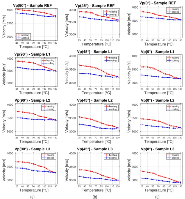
Figure 6 – P-wave velocities ((a) V p90, (b) V p45and (c) V p0) as function of temperature for samples REF, L1, L2 and L3 for heating and cooling cycles.

To estimate P-wave velocities, we used the relation given as:

VP(θ) =

LP

tP(θ) − ∆tdelay

, (2)

where LP is the distance of P-wave propagation, tP(θ) is the

transmission time as a function of the angle with respect to the Z-axis of a P-wave, and ∆tdelayis the delay time due to the S-wave

transducers.

For S-wave velocities, the equation is similar to P-wave. They are given by

VS(φ) =

LS

tS(φ) − ∆tdelay

, (3)

where LS is the distance of S-wave propagation, tS(φ) is the

transmission travel time as a function of the angle polarization. For experimental velocities estimation, it was considered errors due to measurements of length (margin of error = ± 0.02 cm) and time travel picking (margin of error = ± 0.02 microsecond (µs)). The uncertainties for P- and S-wave

25 40 55 70 85 100 115 130 Temperature [°C] 1800 2000 Velocity [m/s] 25 40 55 70 85 100 115 130 Temperature [°C] 1800 2000 2200 2400 Velocity [m/s] V S1 - Sample L2 heating cooling 25 40 55 70 85 100 115 130 Temperature [°C] 1800 2000 2200 2400 Velocity [m/s] V S1 - Sample L3 heating cooling (a) 25 40 55 70 85 100 115 130 Temperature [°C] 1800 2000 Velocity [m/s] 25 40 55 70 85 100 115 130 Temperature [°C] 1800 2000 2200 2400 Velocity [m/s] V S2 - Sample L2 heating cooling 25 40 55 70 85 100 115 130 Temperature [°C] 1800 2000 2200 2400 Velocity [m/s] V S2 - Sample L3 heating cooling (b)

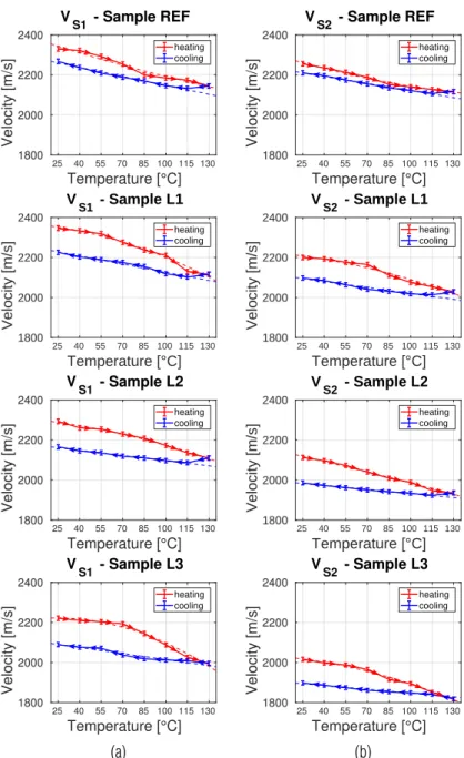
Figure 7 – S-wave velocities ((a) Vs1and (b) Vs2) as function of temperature for samples REF, L1, L2 and L3 for heating and cooling cycles.

velocities estimate ranged from ± 20 to ± 35 m/s and ± 18 to ± 28 m/s. Related to the temperature, the margin of error was ± 5◦_{C for both heating and cooling process.}

RESULTS

Figures 6 and 7 show, respectively, the variation of P- and S-wave velocities as a function of temperature, for all propagation and polarization directions. They are related to all the samples in study and show the behavior of compressional and shear velocities during both the heating (red curves) and cooling (blue curves) of

samples. For all the cases it is observed a decrease in velocities with the increasing temperature. Also, it is evident the existing of hysteresis in all the samples for all velocities, i.e., there is a variation of velocity for the same temperature when the sample is heating and cooling. Using the support of previous works to interpret these behaviors, such as the works of Timur (1977), Kern (1978) and Jansen et al. (1993), it can be said that they may be caused by the generation of microcracks inside the samples (secondary cracking), the coalescence of those microcracks and the decrease of the background stiffness of the samples. As

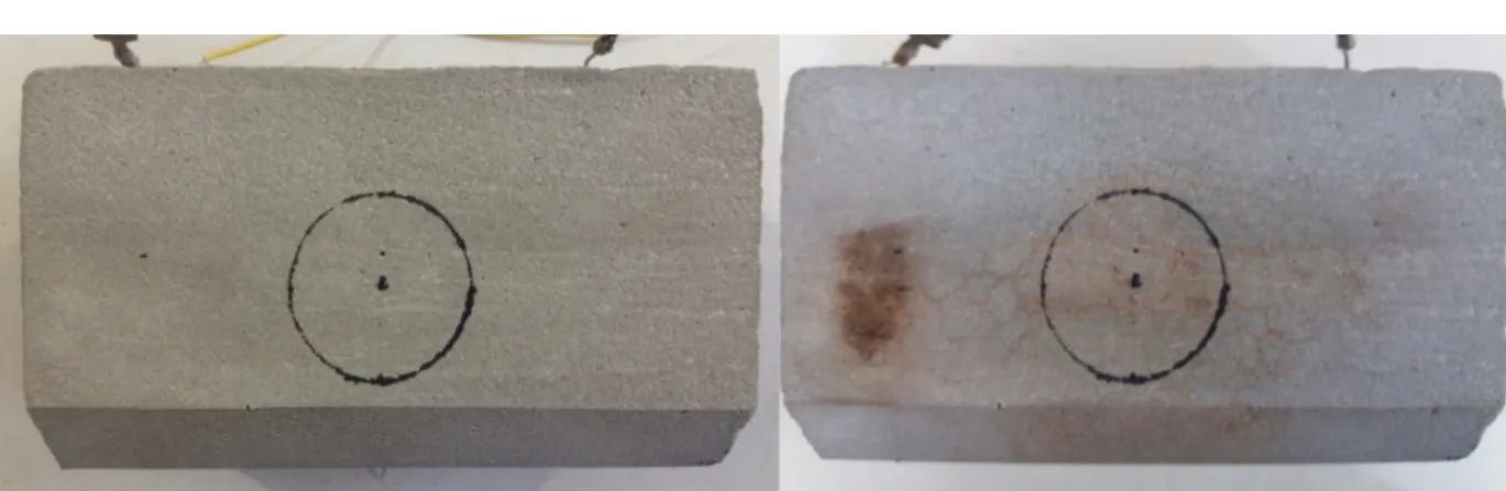
Figure 8 – Sample L2 before and after heating. It can be seen the presence of fissures on the surface caused by the coalescence of microcrasks. 3000 L3 3500 L2 Velocity [m/s] Sample 4000 130 115 L1 Vp(90o₎ 100 Temperature [°C] 85 70 4500 55 40 25 REF 3300 3400 3500 3600 3700 3800 3900 4000 (a) 3000 L3 L2 Sample 130 115 100 Temperature [ o_C] 85 L1 70 3500 55 Velocity [m/s] 40 25 Vp(45o₎ REF 4000 3000 3100 3200 3300 3400 3500 3600 3700 3800 3900 (b) 3000 L3 3500 L2 Sample Velocity [m/s] 130 115 4000 L1 100 Temperature [°C] 85 Vp(0o₎ 70 55 40 25 4500 REF 3000 3100 3200 3300 3400 3500 3600 3700 3800 (c) 1800 L3 L2 2000 Sample Velocity [m/s] L1 2200 130 115 Temperature [ oC] 100 85 70 55 40 S-wave - Vs1 REF 25 2400 2000 2050 2100 2150 2200 2250 2300 (d) 1800 L3 L2 2000 Sample Velocity [m/s] L1 2200 130 115 Temperature [ o_C] 100 85 70 55 S-wave - Vs2 40 REF 25 2400 1850 1900 1950 2000 2050 2100 2150 2200 2250 (e)

Figure 9 – Elastic velocities ((a,b,and c) P and (d and e) S) as function of temperature and crack densities shown by maps graphics. For all maps the highest velocity occurs when the temperature is 25o_{and the crack density is 0. The colorbar unity is m/s.}

expected, the opposite behavior occurs when the samples cooled. Since the microcracks generated by the heating process do not disappear when the samples are cooled down, it can be inferred that the behavior showed by the blue lines, where the velocities increased with the decreasing temperature, are solely or mostly related to the variation of background stiffness. Another indicatives of the secondary cracking and cracking coalescence is the fact that the velocities never return to their initial values after the cooling process and the increasing in porosity for all the

samples after the experiment, as it can be seen in Table 2. The coalescence of microcracks created fissures on the outer edge of the samples, as it can be seen in Figure 8 that shows sample L2 before and after heating. On average, P-wave velocity decreased 11% for a 105◦_{C rise in temperature, whereas S-wave decreased}

on average 9% for the same temperature gradient.

Figure 9 shows the variation of all the velocities as function of both temperature and the crack density, representing by the sample labels. Figure 9 concatenates all velocity data from

Temperature [°C] 25 40 55 70 85 100 115 130 Temperature [°C] 0 0.05 0.1 0.15 0.2 - L1 heating cooling 25 40 55 70 85 100 115 130 Temperature [°C] 0 0.05 0.1 0.15 0.2 - L2 heating cooling 25 40 55 70 85 100 115 130 Temperature [°C] 0 0.05 0.1 0.15 0.2 - L3 heating cooling (a) Temperature [°C] 25 40 55 70 85 100 115 130 Temperature [°C] 0 0.05 0.1 0.15 0.2 - L1 heating cooling 25 40 55 70 85 100 115 130 Temperature [°C] 0 0.05 0.1 0.15 0.2 - L2 heating cooling 25 40 55 70 85 100 115 130 Temperature [°C] 0 0.05 0.1 0.15 0.2 - L3 heating cooling (b) Temperature [°C] 25 40 55 70 85 100 115 130 Temperature [°C] -0.2 -0.1 0 0.1 0.2 - L1 heating cooling 25 40 55 70 85 100 115 130 Temperature [°C] -0.2 -0.1 0 0.1 0.2 - L2 heating cooling 25 40 55 70 85 100 115 130 Temperature [°C] -0.2 -0.1 0 0.1 0.2 - L3 heating cooling (c)

Figures 6 and 7 during the heating process. It can be seen that the gradient of velocity as a function of temperature and crack density points in the direction of minimum temperature and crack density, which is a expected behavior since velocity decreases with increasing temperature and increasing crack density.

Table 2 – Initial porosity, final porosity and secondary crack porosity (after heating and cooling) of all samples used in this study.

Sample Initial Porosity Final Porosity Induced Porosity

REF 8.2% 18.0% 9.8%

L1 12.0% 21.0% 9.0%

L2 14.0% 23.5% 9.5%

L3 15.5% 25.5% 10.0%

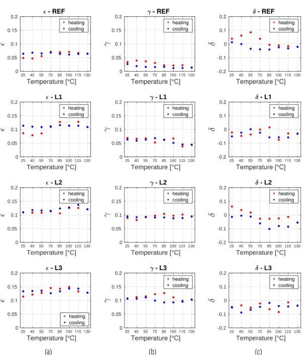
Figure 10 shows the variation of the Thomsen’s parameters (γ, ε and δ) as a function of temperature, for sample L2, during both the heating and cooling processes. Theγ and ε values increase as the number of cracks of the samples increase, which is an expected behavior. In most of the cases, the γ and ε values show very close heating and cooling values, which is consisting with the observations made by Kern & Fakhimi (1975) that temperature does not noticeably reduce fabric-induced anisotropy. This may be caused by the fact that P-wave velocities in the 0◦ _{direction decrease at approximately}

the same rate as the 90◦_{direction; the same occurs for S-wave}

velocities for different polarizations. This is an indicative that the secondary cracks generated during the heating process are randomly oriented. As for theδ parameter, it does not seem to show any correlation with temperature variation.

CONCLUSIONS

An ultrasonic procedure was performed on synthetic samples representing isotropic and cracked sandstones. They were constructed using cheap materials and a very simple construction methodology. The waveforms were acquired from the samples for different temperatures, which was possible by using a temperature controlling system. From the analyzes of the results, the following conclusions were obtained:

• The increasing temperature decreases the background stiffness and generates secondary cracks inside the samples.

• P-wave velocities had on average a 11% decrease for a 105◦_{C rise in temperature, and P-wave velocity decreased}

approximately at the same rate on all directions of propagation.

• S-wave velocities had on average a 9% decrease for a 105◦_{C rise in temperature, decaying at the same rate for}

both polarizations.

• Anisotropy parameters γ and ε presented very close values both for heating and cooling. They do not show a satisfactory pattern with the increasing and decreasing temperature, making their use as tools to model elastic properties as a function of temperature not applicable. In addition, it is worth to highlight the importance of this work as the first approach using porous synthetic rocks in the analysis of the influence of temperature in the behavior of elastic properties. The same approach may be repeated using rocks with different mineralogical composition and/or anisotropy symmetries.

ACKNOWLEDGMENTS

The authors would like to thank SBGf for the scholarship and the Brazilian agencies PET/GEOFÍSICA-UFPA-Ministério da Educação, INCT-GP and CNPq (grant no. CNPq 459063/2014-6 and grant no. CNPq 140174/2016-8) from Brazil and the Geophysics Graduate Program at the Universidade Federal do Pará for the financial support in this research. The authors would also like to thank the reviewers for many helpful comments and suggestions.

REFERENCES

BROTÓNS V, TOMÁS R, IVORRA S & ALARCÓN JC. 2013. Temperature influence on the physical and mechanical properties of a porous rock: San Julian’s calcarenite. Engineering Geology, 167: 117–127. doi: 10.1016/j.enggeo.2013.10.012. URL http: //www.sciencedirect.com/science/article/pii/S001379521300286X. DE FIGUEIREDO JJS, DO NASCIMENTO MJS, HARTMANN E, CHIBA BF, DA SILVA CB, DE SOUSA MC, SILVA C & SANTOS LK. 2018. On the application of the Eshelby-Cheng effective model in a porous cracked medium with background anisotropy: An experimental approach. Geophysics, 83(5): C209–C220.

DE FIGUEIREDO SJJ, SCHLEICHER J, STEWART RR, DAYUR N, OMOBOYA B, WILEY R & WILLIAM A. 2013. Shear wave anisotropy from aligned inclusions: ultrasonic frequency dependence of velocity and attenuation. Geophysical Journal International, 193(1): 475–488. doi: 10.1093/gji/ggs130.

GARCIA GCR, SANTOS EMB & RIBEIRO S. 2011. Effect of the curing time on the stiffness of mortars produced with Portland cement.

93JB01816/abstract.

KERN H. 1978. The effect of high temperature and high confining pressure on compressional wave velocities in quartz-bearing and quartz-free igneous and metamorphic rocks. Tectonophysics, 44(1): 185–203. doi: 10.1016/0040-1951(78)90070-7. URL http://www.sciencedirect.com/science/article/pii/0040195178900707. KERN H & FAKHIMI M. 1975. Effect of fabric anisotropy on compressional-wave propagation in various metamorphic rocks for the range 20-700◦C at 2 kbars. Tectonophysics, 28(4): 227–244. doi: 10.1016/0040-1951(75)90039-6. URL http://www.sciencedirect.com/ science/article/pii/0040195175900396.

MARTÍNES JM & SCHMITT DR. 2011. Investigating anisotropy in rocks by using pulse transmission method. CSEG RECORDER Magazine, p. 38–41. URL https://www.csegrecorder.com/articles/view/investigating-anisotropy-in-rocks-by-using-pulse-transmission-method.

POLETTO M, ORNAGHI JÚNIOR HL & ZATTERA AJ. 2014. Polystyrene: synthesis, characteristics, and applications. In: LYNWOOD C (Ed.). Polystyrene: Synthesis, Characteristics and Applications. New York: Nova Science Publishers, 303, Chapter 3, p. 53–74.

VTI media. In: 15th International Congress of the Brazilian Geophysical Society & EXPOGEF, Rio de Janeiro, Brazil, 31 July-3 August 2017, p. 249–254. Brazilian Geophysical Society. doi: 10.1190/sbgf2017-049. URL https://library.seg.org/doi/abs/10.1190/sbgf2017-049.

THOMSEN L. 1986. Weak elastic anisotropy. Geophysics, 51(10): 1954–1966. doi: 10.1190/1.1442051.

TIMUR A. 1977. Temperature dependence of compressional and shear wave velocities in rocks. Geophysics, 42(5): 950–956. doi: 10.1190/1. 1440774. URL https://library.seg.org/doi/abs/10.1190/1.1440774. YAN F, HAN D, YAO Q & CHEN X. 2016. Seismic velocities of halite salt: Anisotropy, heterogeneity, dispersion, temperature, and pressure effects. Geophysics, 81(4): D293–D301. doi: 10.1190/geo2015-0476.1. URL https://library.seg.org/doi/abs/10.1190/geo2015-0476.1. ZHANG L, MAO X & LU A. 2009. Experimental study on the mechanical properties of rocks at high temperature. Science in China Series E: Technological Sciences, 52(3): 641–646. doi: 10.1007/s11431-009-0063-y. URL https://link.springer.com/article/10.1007/s11431-009-0063-y.

Recebido em 22 setembro, 2018 / Aceito em 25 novembro, 2018 Received on September 22, 2018 / accepted on November 25, 2018