IMPLEMENTING INTEREST RATE SWAPS IN THE RISK MANAGEMENT OF A CREDIT INSTITUTE – A PRACTICAL ANALYSIS
TIM BEERMANN STUDENT NUMBER: 3981
STUDENT ID: 29825
A Project carried out on the Master in Finance Program, under the supervision of: Professor Afonso Fuzeta de Eça
Implementing Interest Rate Swaps in the Risk Management of a Credit Institute –
A Practical Analysis
Abstract
This Work Project has been developed in the course of an internship done at a credit institute and analyzes hedging strategies based on interest rate swaps that enable isolated management of interest rate risk. It follows a practical approach to test five fair value hedges, which are thought to immunize against different term structure shifts. Additionally, a strategy is devised that hedges interest rate risk in forecasted earnings, which is expressed by an earnings shortfall below certain minimum threshold values in different planning scenarios.
List of keywords
Interest rate risk Interest rate swap Immunization Hedging
Contents
Declaration of Originality 4
1. Introduction 5
2. Literature Review 7
3. Data and Methodology 11
4. Results and Discussion 18
5. Summary 24
References 26
Appendix A: Equations 28
1. Introduction
In credit institutes’ line of business interest rate risk usually constitutes one of the most important sorts of risk. This Work Project has been developed in the course of an internship done at a credit institute specializing in real estate financing. The focus of the internship was set on analyzing hedging strategies with interest rate swaps (IRSs) to manage exactly this sort of risk.
At the time of the internship, financial institutes had to control and report the interest rate risk they face, and the utilization of their liable equity held for it, in the two simple interest rate shock scenarios of the Basel Committee on Banking Supervision. Soon it was likely that this spectrum increases by six alternative scenarios to report if the European Banking Authority’s guideline on interest rate risk in the banking book (IRRBB) will finally come into force. For the credit institute hosting the internship, it probably becomes necessary in the future to apply efficient hedging strategies, which can secure the institute’s economic value of equity (EVE) in each scenario. Moreover, the low-interest environment is taking its toll on most of the credit industry and the credit institute’s traditional business model was currently suffering from retrogressive new lending. The surplus long-term funding from the home savings collective as well as the short-term funding was invested into long-term bonds, but not enough risk could be taken on without an unwanted balance sheet extension through further short-term funding, thus putting earnings under pressure. Countering this with the interest rate risk management system in place became very difficult, because, as a traditional credit institute, it has been held on to the conventional methods so far, by using bonds as cash instruments and constantly adjusting the commercial strategy of the credit and home savings collective. But managing the credit and home savings collective is extremely sluggish, with direct control impulses often having an effect only after years. Using cash
instruments is, in theory, more flexible and its control impulses have a faster impact, but it was constrained by the institute’s buy and hold strategy in this case. In addition, the spectrum of bonds allowed to invest in was limited by strict constraints imposed by the institute’s investment policy. This increases the risk of an insufficient supply of investment vehicles available in case of a severe interest rate market movement. Finally, it is in the nature of a cash instrument that its investment is not only exposed to interest rate risk but also to counterparty and liquidity risk, thus making it impossible for the institute to manage interest rate risk without taking on other sorts of risk, increasing the difficulty of the overall risk management system.
Due to the stated disadvantages of the current approach and the challenges ahead, with more scenarios to manage and earnings under pressure, the credit institute wanted to have a tool facilitating an isolated management of interest rate risk, not to fully replace its traditional approach but to be more flexible and to have the chance to react faster. Interest rate swaps should fill this gap, since they bear only interest rate and neither liquidity nor counterparty risk and are accounted off-balance, not leading to any balance sheet extension. But holding on to their traditional approach so far, which was enough and efficient up to now, it was never genuinely thought of a derivatives usage before and the necessary in-house knowledge was non-existent.
To overcome all obstacles the internship set the challenge of testing different hedging strategies available in academic literature in a practical manner within the institute’s business environment to reduce interest rate risk and secure the EVE in all scenarios (fair value hedges), as well as to devise a strategy on how to hedge interest rate risk from an earnings perspective in their profit and loss (P&L) forecasts with interest rate swaps (P&L hedge). The goal of this Work Project has been to model the implementation of swap-based hedging strategies and to evaluate the tested and devised strategies, to derive a thorough recommendation to the credit institute in the end.
2. Literature Review
In the academic literature strategies for hedging interest rate risk have been comparatively well researched in the past decades, building on from the basics of finance towards more sophisticated models. Yet most of the research is purely theoretical and only a few follow a practical approach as it is the focus of this Work Project. Nevertheless, the theoretical findings are the foundation of this analysis, by giving the instructions on how to implement each strategy and enabling the test of their practical applicability. They deviate sometimes more, sometimes less, but all have in common that they construct a hedge portfolio which mirrors some sorts of characteristics of the portfolio to be hedged. Most of the strategies focus on hedging the EVE of a portfolio (fair value hedges), while a practical strategy for hedging an earnings stream (P&L hedge) is devised later in this work. The cash flow matching strategy is probably the most intuitive and straightforward strategy. It can meet a portfolio of multiple interest rate sensitive assets and liabilities by selecting a hedge portfolio of assets and liabilities whose cash flows mirror the cash flows of the assets and liabilities to be hedged (Choudhry, 2003). First, the longest-dated cash flow to be hedged is matched by a fixed-income instrument’s cash flow, which has the same maturity date and the inverse value of the target cash flow and is composed of principal and interest payment. The instrument’s other interest payments are netted with the shorter-dated cash flows to be hedged. Subsequently, the second longest-dated target cash flow, perhaps offset to some extent by the interest payment of the longest-dated hedging instrument, is then matched in the same manner as before with a second hedging instrument. These steps are repeated backward the target cash flow stream so that the shortest-dated cash flow is netted with all interest payments from longer-dated instruments occurring on its maturity date and then finally matched by the last fixed-income instrument needed (Veronesi, 2011). By completing all steps and matching each target cash flow, the portfolio of
assets and liabilities to be hedged is, in theory, completely immunized against shifts of the term structure.
If the quantity of different cash flows stemming from the portfolio increases, the quantity of different maturity dates of the asset and liability items increases accordingly. Each spot rate at the respective maturity date can be seen as a risk variable and the increasing complexity can cause difficulties when hedging many different variables in practice. To alleviate this difficulty other strategies build on reducing the number of risk variables by selecting as little risk variables as possible, which are sufficient to explain changes in the term structure and asset values (Martellini, Priaulet and Priaulet, 2002).
The most traditional strategy following this methodology and likely the most used in real-world applications is the technique of duration hedging. It applies the yield to maturity of the target portfolio as a single risk factor representative for the whole term structure (Martellini, Priaulet and Priaulet, 2003). The duration of the portfolio is its first-order price approximation and a function of the portfolio’s yield to maturity. The value of the portfolio is immunized against changes in interest rates by constructing a hedge portfolio, whose duration equals the inverse duration of the target portfolio and whose value equals the present value of the target portfolio, both discounted at the current term structure (Christensen and Sørensen, 1994). Combining both means nothing else than that the $duration of the hedge portfolio must equal the inverse $duration of the target portfolio for a successful hedge. But relying on the yield to maturity, which is a complex average of the yield curve, imposes the assumption, that changes in the yield curve are parallel shifts only (Fabozzi, 1996), although this condition is barely observed in real life. Moreover, duration, as the first-order price approximation, only holds true for small interest rate shifts, thus further limiting the successfulness of the duration hedge (Choudhry, 2003). Despite these restrictive assumptions, it
was necessary to model and test this strategy, even if inefficiency in real life applications was assumed. Demonstrating the pitfalls of this strategy to the credit institute substantiates the necessity of more complex models and helps to find a reasonable recommendation in the end.
To relax the assumption of small shifts of the term structure only, a convexity term can be added to the duration hedge (Reitano, 1992). The convexity of the portfolio is its second-order price approximation and yields a closer approximation of the value change than it is done by only using duration. Immunization is then achieved by constructing a hedge portfolio, whose $duration and $convexity equal the inverse of the $duration and $convexity of the portfolio to be hedged. But since this duration convexity hedge still relies on the yield to maturity, it is the predominant opinion in the academic literature, that it still suffers from the assumption that changes in the yield curve are of a parallel kind only (various sources, e.g. Reitano, 1992 and Veronesi, 2011). However, hedging duration and convexity require the utilization of two different hedging instruments to serve both portfolio sensitivity figures and the contrary opinion also exists, that a hedge applying two instruments with differing durations can also protect against changes in the slope of the curve and not only parallel shifts (Falkenstein and Hanweck, 1996). Thus, in the further process of this Work Project, it was important to analyze how the duration convexity hedge performs in practice under different interest rate scenarios and which opinion turns out to be more accurate.
To generally relax the assumption of parallel shifts only, one can move away from the traditional measures of duration and convexity towards term structure models with more sophisticated sensitivity figures, which do not rely on the yield to maturity anymore. To get to the heart of hedging efficiency, the better a term structure model approximates reality the better the hedging strategy, based on this model, will perform (Barber and Copper, 1996). One model trying to do so
is the Nelson-Siegel model, which introduces the level (β0), slope (β1) and curvature factor (β2) as well as a decay factor (λ) (Nelson and Siegel, 1987):
𝑟𝑁𝑆(0, 𝑇) = 𝛽0+ 𝛽1 1 − 𝑒−𝑇/𝜆 𝑇/𝜆 + 𝛽2[ 1 − 𝑒−𝑇/𝜆 𝑇/𝜆 − 𝑒 −𝑇/𝜆] (1) The level factor β0 represents the long-term interest rate and can be linked to parallel shifts of the curve. A steepening or flattening of the curve is captured by the slope factor β1, which decays exponentially if maturity increases. The curvature factor β2 captures humps in the curve and rises towards the middle of the maturity spectrum (Barrett, Gosnell and Heuson, 1995). These three factors account for most of the changes in the term structure (Litterman and Scheinkman, 1991). Overall, the Nelson-Siegel model allows for multi-dimensional interest rate changes and so does the Nelson-Siegel hedge. It is performed by calibrating the model factors and measuring the level, slope and curvature $durations of the portfolio to be hedged, so that a hedge portfolio with the inverse $durations can be constructed with three hedging instruments.
The Svensson model extends the Nelson-Siegel model by a second curvature (β3) and decay factor (λ2), thus allowing even more flexibility in estimating the yield curve and more complex curves like hump- and U-shaped ones (Svensson, 1994):
𝑟𝑆𝑣(0, 𝑇) = 𝛽0+ 𝛽1 1 − 𝑒−𝑇/𝜆1 𝑇/𝜆1 + 𝛽2[ 1 − 𝑒−𝑇/𝜆1 𝑇/𝜆1 − 𝑒−𝑇/𝜆1] + 𝛽3[1 − 𝑒 −𝑇/𝜆2 𝑇/𝜆2 − 𝑒−𝑇/𝜆2] (2)
The hedging is then executed analog to the Nelson-Siegel hedge, just with four different hedging instruments. Due to its flexibility and sophistication, one could expect the best results and hedging efficiency delivered by this strategy. In the further process of this work, it had to be verified if the Svensson hedge is indeed the optimum fair value hedge for the credit institute and if not, which one of the presented strategies might do better for their needs and outperforms the expectations.
3. Data and Methodology
The analysis’ starting point is the utilization of liable equity. With an upper limit of 20% imposed by regulatory authorities, the credit institute wants to follow a target utilization of 15%. The real utilization has been 10,5%, giving it the opportunity to load up more risk (from a present value perspective) to generally increase earnings and to hedge earnings in the worst-case planning scenario (P&L hedge). For the possible situation that the real utilization would be above the target utilization, the institute wanted to have different fair value hedging strategies investigated (Figure 1). So only for comparison purposes, the fair value hedging strategies should fully hedge interest rate risk, which corresponded to a 100% degree of hedging and utilization of 0%.
The company data needed for the analysis was manually altered due to confidentiality reasons but still reflects the institute’s characteristics and situation. Besides the base interest rate scenario there are eight interest rate scenarios for measuring interest rate risk from a present value perspective, which are assumed to instantly occur on the time of the analysis as shifts of the term structure:
+200 bps and -200 bps (Basel interest rate shock, see Figure 2) and a parallel up PU, parallel down PD, steepening ST, flattening FL (slight inverse curve after altering due to confidentiality reasons),
short up SU and short down SD scenario (IRRBB scenarios, see Figure 3). There are also three planning scenarios with forecasted yield curves for simulating future earnings (P&L): a base planning scenario, an interest rate reduction scenario and an interest rate increase scenario. These two kinds of scenarios do not interfere, and it must be rigorously distinguished between both in the further process of this work. Furthermore, the sum of liable equity, daily cash flows, earnings before taxes (EBT) in each planning scenario (Figure 4) and the interest rate sensitive balance sheet items with their durations, convexities and present values in each interest rate scenario, were provided. Finally, market rates for IRSs (bid/ask) and EURIBOR 3M were obtained from Reuters.
Using the daily cash flows given would have required one IRS at each date of occurrence in the cash flow matching strategy and one interest rate at each date of occurrence in the Nelson-Siegel and Svensson hedge. To avoid this quantity of swaps and interest rates, the forecasted cash flow stream of the next 20 years (credit institute’s standard simulation horizon) was mapped to a quarterly basis. This scheme is relative to the day of analysis and not necessarily to calendar quarters, which therefore complies with the more frequently traded swap maturities in the market (quarters and whole years). The mapping was done in two different ways, a periodic mapping with all daily cash flows mapped onto the last day of the current quarter and a linear mapping with each daily cashflow linearly distributed between the preceding and the current quarter (Equation 3). Where they were missed, the quarterly swap rates for the cash flow matching and the interest rates for the swap valuation were both linearly interpolated (Ron, 2000), which was in line with the credit institute’s standard (Equation 4). The final valuation in each strategy was then made for plain vanilla interest rate swaps with EURIBOR 3M-floating legs, which were solely used for the analysis. These swaps can be easily replicated by going long and short one fixed-rate bond and one floating-rate bond, both with the same nominal so that their value is the difference of both bond values (Hull, 2012). In the same manner, the duration and convexity of the plain vanilla interest rate swap is the difference of the durations and convexities of both bonds (Equations 5-7).
The total value of all swaps in each strategy’s hedge portfolio varies accordingly to the simulated interest rate scenario of which the discount factors were obtained. Depending on the scenario, the total value contributes positively or negatively to the present value of the credit institute’s whole portfolio (Beets, 2004), hence the credit institute’s EVE. The change in EVE (∆EVE) in each interest rate scenario reflects the static interest rate risk each strategy (of the fair value hedges) aims to neutralize. The absolute value of the worst ∆EVE over all eight interest rate scenarios is the
scenario method’s static value at risk (VaR). In general, this VaR must be minimized and is the main ingredient of the efficiency measure for each strategy (of the fair value hedges). As stated before, the efficiency of each fair value hedge is measured at a 100% degree of hedging and should lie between 80% and 125%, to consider a strategy as efficient (FBE, 2003):
𝑒𝑓𝑓𝑖𝑐𝑖𝑒𝑛𝑐𝑦100%=
𝑉𝑎𝑅0%+ 𝑚𝑖𝑛100%(∆𝐸𝑉𝐸+200 𝑏𝑝𝑠, ∆𝐸𝑉𝐸−200 𝑏𝑝𝑠, … , ∆𝐸𝑉𝐸𝑆𝑈, ∆𝐸𝑉𝐸𝑆𝐷)
𝑉𝑎𝑅0% (8)
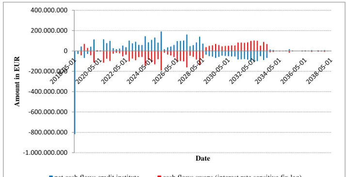
After finishing all necessary auxiliary calculations, the cash flow matching is executed as described before in the literature review, but instead of bonds, the fixed leg of interest rate swaps is used for the determination of the swaps needed. The floating leg is disregarded, because in this technique, the interest rate sensitive cash flows of the credit institute are only matched by the interest rate sensitive principal and interest payments of the fix leg of the IRS, which are in fact pseudo cash flows of the IRS, since the principal of the fix leg/nominal of the swap is not really exchanged (Figure 5 and 6). The strategy was tested for the credit institute’s standard simulation horizon of 20 years with both, the periodic mapped and the linear mapped quarterly cash flows, which required 79 swaps (20 years x 4 quarters – 1st quarter owing to the minimum swap maturity of a half year). Due to the practical approach of the work, precise nominals modeled were in this and every other strategy ultimately rounded to tenths of millions to ensure the tradeability of the swaps.
Compared to the cash flow matching, the strategies relying on sensitivity figures like duration or convexity do not have a fixed set of specific swap maturities needed. For these remaining fair value hedging strategies, all possible maturity combinations with swaps maturing between 1 and 20 years (only full years) were calculated. It is important for the duration convexity, Nelson-Siegel and Svensson hedge (all with >1 hedging instrument), that the maturity of a shorter-term IRS is always smaller and never equal to the maturity of a longer-term IRS so that there are enough IRSs with
differing sensitivities to mirror the institute’s portfolio. This leads to 20 combinations for the duration hedge, 190 for the duration convexity hedge, 1140 for the Nelson-Siegel hedge and 4845 for the Svensson hedge, which differ in their efficiency and the total nominal needed.
The duration hedge, as the first of those remaining strategies, starts with the determination of the target portfolio’s $duration, which is the sum of the products of each balance sheet item’s duration and present value in the base interest rate scenario. A positive $duration is offset by the negative $duration of a payer-swap, a negative one by applying a receiver-swap. The hedge ratio ϕ is
𝜙 = −∑ 𝑝𝑟𝑒𝑠𝑒𝑛𝑡 𝑣𝑎𝑙𝑢𝑒 (𝑖𝑡𝑒𝑚𝑖) × 𝑑𝑢𝑟𝑎𝑡𝑖𝑜𝑛𝑖 $𝑑𝑢𝑟𝑎𝑡𝑖𝑜𝑛𝐼𝑅𝑆
= −$𝑑𝑢𝑟𝑎𝑡𝑖𝑜𝑛𝑝𝑜𝑟𝑡𝑓𝑜𝑙𝑖𝑜
$𝑑𝑢𝑟𝑎𝑡𝑖𝑜𝑛𝐼𝑅𝑆 (9)
where $durationIRS is the $duration of a payer, respectively receiver swap, that is standardized with a swap nominal of EUR 1.000.000. In the duration convexity hedge, the added $convexity term is determined analogously to the $duration term, whereas the calculation of the hedge ratio ϕi, with the swaps needed for each maturity combination, follows
(𝜙1
𝜙2) = Ω𝐷𝐶 ℎ𝑒𝑑𝑔𝑒
−1 × 𝛿
𝐷𝐶 ℎ𝑒𝑑𝑔𝑒 (10)
where ΩDC hedge is a quadratic matrix containing the $durations of the two swaps needed in the first row and their $convexities in the second row, and where δDC hedge is a vector containing the target portfolio’s inverse $duration and $convexity, to offset both sensitivity figures.
On the contrary, modeling the Siegel hedge starts with the determination of the Nelson-Siegel model factors. The equation of the Nelson-Nelson-Siegel model (Equation 1) is estimated over each point in time of the base interest rate scenario and is calibrated according to the least squared error criterion by numerically optimizing the set of β and λ factors (Willner, 1996), so that it best approximates the corresponding interest rate from the base scenario (Figure 7):
min
𝛽0,𝛽1,𝛽2,𝜆
∑[𝑟(0, 𝑇)𝑏𝑎𝑠𝑒 𝑠𝑐𝑒𝑛𝑎𝑟𝑖𝑜− 𝑟(0, 𝑇)𝑁𝑆]2 (11)
The level $duration D0, the slope $duration D1 and the curvature $duration D2 are then defined as
{ 𝐷0= − ∑ 𝑇 × 𝐶𝐹𝑇× 𝑒−𝑇×𝑟𝑁𝑆(0,𝑇) 𝐷1= − ∑ 𝑇 × [ 1 − 𝑒−𝑇/𝜆 𝑇/𝜆 ] × 𝐶𝐹𝑇× 𝑒 −𝑇×𝑟𝑁𝑆(0,𝑇) 𝐷2= − ∑ 𝑇 × [ 1 − 𝑒−𝑇/𝜆 𝑇/𝜆 − 𝑒 −𝑇/𝜆] × 𝐶𝐹 𝑇× 𝑒−𝑇×𝑟𝑁𝑆(0,𝑇) (12)
and measured for the fixed leg of the swaps, as well as for the periodically mapped and linearly mapped quarterly cash flows of the credit institute (Martellini, Priaulet and Priaulet, 2003). For the same reason as for the cash flow matching strategy, the $durations are only calculated for the fixed leg of the swaps. The hedge ratios are determined in the same way as in Equation 10, but now with three IRSs and ΩNS hedge and δNS hedge containing the level, slope and curvature $durations of the swaps’ fix legs and the inverse $durations of the mapped cash flows. Implementing the Svensson hedge follows the same actions that are necessary for the Nelson-Siegel hedge (Figure 8), by minimizing the error
min
𝛽0,𝛽1,𝛽2,𝛽3,𝜆1,𝜆2
∑[𝑟(0, 𝑇)𝑏𝑎𝑠𝑒 𝑠𝑐𝑒𝑛𝑎𝑟𝑖𝑜− 𝑟(0, 𝑇)𝑆𝑣]2 (13)
and extending the matrix multiplication with a forth IRS and the second curvature $duration of the Svensson model, which is calculated with the second decay factor λ2
𝐷3= − ∑ 𝑇 × [
1 − 𝑒−𝑇/𝜆2
𝑇/𝜆2
− 𝑒−𝑇/𝜆2] × 𝐶𝐹𝑇× 𝑒−𝑇×𝑟𝑆𝑣(0,𝑇) (14)
to ultimately get the set of four different interest rate swaps that fully immunizes against even large and unparallel shifts of the term structure.
Finally, after modeling the five fair value hedges, the focus of the analysis is now primarily set on the profit and loss statement. The P&L hedge is explained by means of the credit institute’s company data. It can be easily implemented in other institutes and situations, too, but a real utilization of liable equity below the target utilization is always necessary. The credit institute measures its interest rate risk from the earnings perspective by simulating a reduced P&L over 20 years in the three different planning scenarios (not: interest rate scenarios to measure interest rate risk from a present value perspective). The starting point of the strategy is the worst-case planning scenario, which has been the interest rate reduction scenario in this case. The institute’s goal was to at least offset the negative EBTs in the years in which they occur in the worst-case scenario. In general, depending on the size of the difference between real and target utilization of liable equity, which constitutes nothing else than a present value interest rate risk buffer, the P&L hedge can freely alter the EBT in the desired manner in each year.
To do so, the P&L hedge requires the optimization of a hedge portfolio of 20 swaps with maturities from 1 to 20 years, covering each of the simulated years. The swaps’ nominals range, in theory, from -∞ to +∞ and are the only variables to change. The sides of the swaps needed (payer or receiver) are determined by the signs of the swap nominals, reducing the variables to be changed from 40 to 20. The hedge portfolio’s return in form of the compound interest payments is calculated for each year with the fixed swap rates obtained from the market data and the floating swap rate obtained from the forecasted 3-months rate of the worst-case planning scenario. The fixed rates depend on the sides of the swaps, thus taking the costs of the strategy, inherent in the bid-ask spreads, into account. The optimization of the hedge portfolio is finally conducted by simultaneously changing the 20 variables/swap nominals within their boundaries and aims to either minimize the total nominal needed or to maximize the total hedge portfolio’s return (Equation 15).
In both cases, the optimization is subject to inevitable constraints. Firstly, in each year, it is necessary that the compound interest payments must be equal to or larger than a predefined minimum amount. In this case, it is the inverse EBT from the worst-case planning scenario, so that any negative EBT can be avoided (must be modified according to the situation or intentions). Like this, simulated negative EBTs are offset by the hedge portfolio’s positive return and simulated positive EBTs will not drop below zero if the hedge portfolio’s return is negative. It is important that these minimum amounts are defined with enough leeway so that a solution can be found in the optimization procedure. Secondly, the total value of the hedge portfolio must be equal to or larger than the inverse of the present value interest rate risk buffer in absolute terms, measured in the +200 bps and -200 bps interest rate scenarios (here: present value perspective; not: planning scenarios), which is the interest rate shock currently required by authorities (IRRBB scenarios can be added, if necessary). Like this, the interest rate risk buffer of 4,5% in this case (15% target utilization – 10,5% real utilization) is not exceeded and the target utilization is achieved. By setting the condition to “equal or larger”, although the exact target utilization shall be achieved, more flexibility is given into the optimization. In general, by aiming to neutralize the negative EBTs or to achieve another desired hedge portfolio’s return, the interest rate risk buffer is automatically (almost perfectly) exploited to the fullest extent possible. Setting the condition only to “equal” to achieve an exploitation precisely down to the last euro, the variables tend to show unreasonable values. Lastly, and only valid for the optimization aiming to maximize the hedge portfolio’s return, the total nominal over all swaps can be equal to or smaller than a maximum total swap nominal if wanted. In this case, it had to be equal to or less than three billion euros, which constitutes about one third of the credit institute’s balance sheet total. In the end, the efficiency of the strategy is tested by visual inspection. Therefore, the determined swap nominals are rounded to ensure better tradeability and interest rate payments are recalculated and added to the forecasted EBT.
4. Results and Discussion
For pursuing a target utilization of liable equity, the credit institute’s overall goal was to find two efficient strategies, one to hedge the forecasted P&L while loading up interest rate risk in the present value perspective (-∆EVEscenarios) and a second one, in turn, to decrease interest rate risk in
the latter. This goal was subject to two restrictions imposed by business policy and shareholders, namely keeping swap nominals as low as possible and utilizing only interest rate swaps and no other derivatives. The following Table 1 sums up the results of the cash flow matching strategy, which is the only fair value hedging strategy with a fixed set of swaps, total nominal and efficiency, and will thus serve as a benchmark against which all other strategies will be compared:
Table 1: Cash flow matching statistics
Efficiency Total nominal
Linear mapping 88,1% 4.374
Periodic mapping 94,9% 4.593
Total nominal in EUR millions.
With both kinds of cash flow mapping, the cash flow matching was generally efficient in all interest rate scenarios, although the hedge with periodic mapping significantly outperformed the one based on linear mapping. This difference was due to the minimum IRS maturity of a half year. In the periodic mapping, all daily cash flows occurring after the first quarter (>0,25 years) were mapped to the end of the second quarter (0,5 years) and could thus be hedged. The linear mapping distributed those daily cash flows in part to the end of the first quarter, which then caused the lesser total nominal and efficiency. To solve the problem of the minimum swap maturity in both cases, the credit institute would have had to utilize a floating rate agreement (FRA), for example, to hedge the mapped cash flow at the end of the first quarter, but this would have been against the restriction of only using interest rate swaps. Using, in theory, daily instead of mapped cash flows, would have
brought the cash flow matching strategy up to almost perfect efficiency, but would have required an unreasonable quantity of hedging instruments. To get to the heart of the cash flow matching and every other hedging strategy relying on cash flows, the strategies’ efficiency inevitably relies on the validity of the forecasted (and mapped) cash flows. Lastly, the rounding of the modeled swap nominals caused slight imperfections, but the repercussions were negligible and affected all strategies tested so that this technicality did not compromise the comparison.
For the rest of the analysis, the cash flow matching based on the more efficient periodic mapping was set as the benchmark. Table 2 compares the maximum efficiency possible of all strategies with unlimited total nominal (second column), and while utilizing maximally the total nominal of the cash flow matching strategy (fourth column) as well as the minimum total nominal that other strategies need to achieve at least the same efficiency as the cash flow matching (sixth column):
Table 2: Fair value hedges’ statistics
maximum efficiency with uncon-straint total nominal total nominal needed maximum efficiency with constraint total nominal total nominal needed minimum total nominal to achieve efficiency of cash flow matching exact efficiency achieved
Cash flow matching, p.m. 94,9% 4.593 94,9% 4.593 4.593 94,9%
Duration hedge 37,0% 3.756 37,0% 3.756 N/A N/A
Duration convexity hedge 89,3% 3.418 89,3% 3.418 N/A N/A
Nelson-Siegel hedge, l.m. 94,6% 10.823 92,1% 4.326 N/A N/A
Nelson-Siegel hedge, p.m. 98,1% 19.812 97,4% 4.429 2.402 95,1%
Svensson hedge, l.m. 94,9%* 47.780* 92,2% 4.333 N/A* N/A*
Svensson hedge, p.m. 99,1% 8.700 97,0% 4.553 2.550 95,3%
With l.m. = linear mapping, p.m. = periodic mapping and total nominals in EUR millions. * Data cleaned of abnormal values not reflecting reality.
With its single hedging instrument, the duration hedge could not achieve the efficiency of the cash flow matching with lesser total nominal or exceed the efficiency of the cash flow matching with
the same total nominal. The duration hedge underperformed significantly in this analysis and was the only one of the strategies tested, that had to be considered as generally inefficient (efficiency <80%). It failed to immunize against large or non-parallel shifts of the term structure (Figure 9), which was thus in line with the findings of the academic literature. The maximum risk reduction of only 37% was accomplished by applying an IRS with a maturity of one year. When increasing the swap maturity, the higher $durations of the swaps allowed for smaller total nominals. Simultaneously, the efficiency decreased steadily and at maturities above seven years the hedge even worsened the VaR, thus reversing the initial intention of reducing risk, because the higher $durations caused higher sensitivities of the swap value to unfavorable shifts of the term structure. Whereas the short and medium-term swaps still added little to no value, longer-term swaps worsened the ∆EVE, and hence the VaR, in the hump-shaped and slight inverse interest rate scenarios, as well as in the asymmetrical -200 bps interest rate shock scenario, due to their negative valuation in these more extreme scenarios.
Compared to the duration hedge, the convexity term added in the duration convexity hedge improved the efficiency immensely. But against the predominant opinion in the academic literature, the increase in efficiency was not only caused by better immunizing against the large parallel term structure shifts but also and especially against the asymmetric and non-parallel ones. For the hedge construction, shorter-term swaps with maximum maturities of four years and longer-term swaps, whose maturities exceeded the one of the shorter-term swaps by at least four years, were needed to be efficient while utilizing only a reasonable amount of total nominal. The maximum efficiency of 89% was achieved by combining a 3-year payer-swap (EUR 2,9 billion nominal) and an 11-year receiver-swap (EUR 0,5 billion nominal). This was perfectly in line with Falkenstein and Hanweck’s statement (1996) that two or more hedging instruments with significantly different
durations can protect against changes in the slope of the yield curve and not against parallel shifts only. The overweight of short-term payer-swaps was needed to capture the hump in the short up, the slight U-shape in the short down and the strong kink in the asymmetric -200 bps interest rate shock scenario, which all occurred within the first five years, as best as possible. Although the duration convexity hedge tried to explain as much change as possible in the asymmetric and non-parallel term structure shifts not only through changes of the level (non-parallel shifts) but also through changes of the slope of the curve, it could not capture curvature changes by itself, leaving a significant residual interest rate risk of 11% of the initial VaR. The results of this practical analysis endorsed Falkenstein and Hanweck’s opinion (1996), which ultimately turned out to be true in the circumstances of this Work Project and contradicted the predominant opinion in the academic literature (e.g. Reitano, 1992 and Veronesi, 2011). Overall, the duration convexity hedge must have been considered as generally efficient, but, although less total nominal was needed compared to the cash flow matching strategy, it considerably failed to reach the efficiency of the cash flow matching strategy by trying to explain term structure movements by only one risk variable, the yield to maturity of the target portfolio.
By moving towards the more sophisticated level, slope and curvature factors of the Nelson-Siegel hedge a remarkable increase in hedge efficiency could be achieved. Here, the periodic mapping of the cash flows clearly outperformed the linear mapping again. Compared to the cash flow matching, both mappings could fully capture the risk stemming from the cash flows in the first and second quarter. But since the amount of the credit institute’s very short-term funding depends on the liquidity needs for the next weeks, its maturity is more or less unknown and is therefore usually set to one day by the institute for simulation purposes. Hence, interest rate risk, expressed in form of $durations, was underestimated when this cash flow was linearly mapped. Additionally, by
assigning each cash flow an equal or slightly longer maturity, the periodic mapping is a generally more conservative approach compared to the linear mapping. Both aspects combined ultimately led to lower $durations and thus a slight underestimation of interest rate risk in the linear mapping. Overall, the three factors of the Nelson-Siegel hedge with periodically mapped cash flows almost perfectly captured every term structure change, even in the more extreme scenarios, thus yielding a nearly perfect hedge of 98,1%, while only applying three IRSs. With an equal total nominal, it was more efficient than the cash flow matching, and, even more important, needed almost only half of the total nominal to achieve the same efficiency of the cash flow matching.
The Svensson model should allow for even more flexibility and more complex curves (Svensson, 1994), but the results of the Svensson hedge (with both linear and periodic mapping) reflected this only to a minor extent because the Nelson-Siegel hedge already captured all interest rate changes almost perfectly. The Svensson hedge with a periodic mapping, which was again the superior mapping due to the same reasons as stated above, was generally more efficient than the Nelson-Siegel hedge, but only by 1%. Nevertheless, it failed to exceed the efficiency that the Nelson-Nelson-Siegel hedge achieved by only using the total nominal of the cash flow matching and, more importantly, needed about EUR 150 million more total nominal than the Nelson-Siegel hedge to achieve at least the efficiency of the cash flow matching strategy, due to serving four rather than three IRSs. Ultimately, closing the review of the fair value hedges, the P&L hedge as the devised strategy for hedging the forecasted earnings was tested with both optimizations, minimizing the total nominal needed and maximizing the total earnings. Both were solvable without breaching any of the constraints imposed and as expected, yielded significantly different results according to their intentions, which can be clearly seen in Table 3. In both optimization procedures, the P&L hedge fully exploited the interest rate risk buffer and thus achieved the target utilization of liable equity.
Table 3: P&L hedge statistics
Total nominal optimization Total earnings optimization
Interest rate risk buffer fully exploited fully exploited
Total nominal 2.065 3.000
Total earnings in
Base scenario 57 101
Interest rate reduction scenario 71 121
Interest rate increase scenario -28 -13
All values in EUR millions.
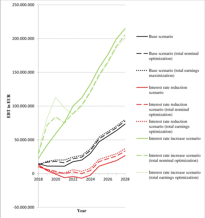
Loading up this present value interest rate risk was rewarded with the desired swap returns, which could be clearly seen by visual inspection (Figure 10). The strategy was efficient by offsetting the negative EBTs in all years in which they occur in the interest rate reduction scenario and generally improving the overall earnings in the base scenario. It cost slightly in the interest rate increase scenario, where EBTs were very high anyway so that it would not have hurt the credit institute. In the situation at hand the interest rate risk buffer has been large enough, but if this is generally not the case, it might be possible, that the negative EBTs cannot be offset or target returns not be achieved, that earnings at the long end of the simulation decrease sharply to balance out necessary high returns with earlier occurrence, or that target returns must be decreased in the first place. In the end, it must be considered that the interest rate scenarios are assumed to instantly occur and to remain constant for the rest of the scenario term, which does not reflect reality. Here, interest rates continuously change and the assets, liabilities and swaps in the portfolio might also be differently sensitive to the passing of time, leading to dissimilar changes of the items’ duration and convexity over time (Christensen and Sørensen, 1994). Hence, the portfolio is hedged against instantaneous shifts of the term structure but not against the passing of time, substantiating the necessity to regularly rebalance the hedged portfolio. Here, a quarterly rebalancing is to favor in reality, due to the transaction costs in the swap market (Dynkin, Hyman and Lindner, 2002).
5. Summary
The analysis on how to implement swaps in the credit institute’s risk management covered five fair value hedges as well as a devised strategy for hedging the forecasted earnings. The cash flow hedge with periodically mapped cash flows yielded a high risk reduction but is impractical in real life application, not only due to the high amount of total nominal needed but especially due to the number of swap transactions necessary and their transaction costs. The inefficient duration hedge, although very much used in practice, could not be considered applicable and substantiated the necessity of more sophisticated models when trying to explain all term structure movements by means of a few variables. The duration convexity hedge was efficient and performed better than predicted by the predominant opinion in the academic literature, but it could not compete with the performance of the Nelson-Siegel hedge, which yielded a nearly perfect hedge in every scenario if based on periodically mapped cash flows. The Svensson hedge added little to no value compared to the Nelson-Siegel hedge, while always utilizing more total swap nominal. Because the scenarios already contained complex curves, the Svensson hedge’s higher flexibility was not expected to become a major advantage in the future anymore. Hence, the Nelson-Siegel hedge was ultimately recommended to the credit institute, since it is easy to implement and rebalance with its three hedging instruments and required the smallest amount of total nominal, while still achieving high degrees of hedging efficiency. In combination to that, the devised P&L hedge was highly recommended, which turned out to be working faultlessly in this context and allowed the desired tradeoff between the higher earnings wanted and the increase of present value interest rate risk, while only utilizing a manageable amount of total nominal despite a hedge portfolio of 20 swaps. In the end, the credit institute was provided with two techniques enabling it to control fast and flexibly its exposure to interest rate risk on an isolated basis, without any balance sheet extension.
Knowledge was delivered on how to achieve the strongly desired increase in earnings with IRSs in the current pressured situation. In case needed, the Nelson-Siegel hedge, in turn, efficiently reduces interest rate risk in all potential scenarios, while only utilizing as little total nominal as possible. To implement both on a regular basis the credit institute was provided with a fully dynamic model, which determines the swaps needed according to the current situation and the institute’s intentions. Before each rebalancing, the model should be used to quickly verify the strategies recommended to ensure that the results of the analysis are still valid. The analysis conducted in this Work Project is a snapshot, based exemplary on the company data as of May 31, 2018. Due to the lack of the time that would have been needed to alter all past original data consistently in the same manner, the analysis was not repeated with data of past years, but its validity is nevertheless unpersuaded. Firstly, the credit institute’s very long-term oriented business model caused only small changes in terms of balance sheet structure, durations, et cetera in the past years, so that the fundamental data on which the analysis is based and hence the analysis’ results as well, would not have been changed much, too. Lastly, due to confidentiality reasons, the original data was altered multiple times until the new fictitious data fully disguised the original data and the credit institute behind it, but still reflected the current situation and the institute’s characteristics. With each of the multiple alterations, the initial analysis was repeated, and each repetition confirmed the results of the initial analysis and no changes were observable that could indicate invalidity of the results.
To deepen the analysis in the future, the implementation of interest rate swaptions can be evaluated in a second step, since the strategies presented only hedge static interest rate risk. Although interest rate risk from optionality makes up only a small amount of the credit institute’s total interest rate risk and is later added to the static interest rate risk for reporting purposes, swaptions would extend the toolset of the institute’s risk management and give it even more flexibility.
References
Barber, Joel R., and Mark L. Copper. 1996. “Immunization Using Principal Component
Analysis.” Journal of Portfolio Management, 23 (1): 99-105.
Barrett, W. Brian, Thomas F. Gosnell, and Andrea J. Heuson. 1995. “Yield Curve Shifts and
the Selection of Immunization Strategies.” Journal of Fixed Income, 5 (2): 53-64.
Beets, Soretha. 2004. “The Use of Derivatives to Manage Interest Rate Risk in Commercial
Banks.” Investment Management and Financial Innovations, 1 (2): 60-74.
Choudhry, Moorad. 2003. The Bond and Money Markets: Strategy, Trading, Analysis. Oxford:
Butterworth-Heinemann.
Christensen, Peter Ove, and Bjarne G. Sørensen. 1994. “Duration, Convexity, and Time Value.” Journal of Portfolio Management, 20 (2): 51-60.
Dynkin, Lev, Jay Hyman, and Peter Lindner. 2002. “Hedging and Replication of Fixed-Income
Portfolios.” Journal of Fixed Income, 11 (4): 43-63.
Fabozzi, Frank J. 1996. Bond Portfolio Management. New Hope, Pennsylvania: Frank J. Fabozzi
Associates.
Falkenstein, Eric, and Jerry Hanweck. 1996. “Minimizing Basis Risk from Nonparallel Shifts
in the Yield Curve.” Journal of Fixed Income, 6 (1): 60-68.
Fédération bancaire de l’Union européenne (FBE). 2003. Macro hedging of interest rate risk.
Brussels: Fédération bancaire de l’Union européenne (FBE).
Hull, John C. 2012. Options, Futures, and Other Derivatives. Harlow, England: Pearson
Litterman, Robert B., and Josè Scheinkman. 1991. “Common Factors Affecting Bond Returns.” Journal of Fixed Income, 1 (1): 54-61.
Martellini, Lionel, Philippe Priaulet, and Stéphane Priaulet. 2002. “Beyond Duration.” Journal of Bond Trading and Management, 1 (2): 103-119.
Martellini, Lionel, Philippe Priaulet, and Stéphane Priaulet. 2003. Fixed-Income Securities: Valuation, Risk Management and Portfolio Strategies. Chichester, England: John Wiley & Sons.
Nelson, Charles R., and Andrew F. Siegel. 1987. “Parsimonious Modeling of Yield Curves.” Journal of Business, 60 (4): 473-489.
Reitano, Robert R. 1992. “Non-Parallel Yield Curve Shifts and Immunization.” Journal of Portfolio Management, 18 (3): 36-43.
Ron, Uri. 2000. “A Practical Guide to Swap Curve Construction.” Bank of Canada Working Paper
2000-17.
Svensson, Lars E. O. 1994. “Estimating and Interpreting Forward Interest Rates.” CEPR
Discussion Paper 1051.
Veronesi, Pietro. 2011. Fixed Income Securities: Valuation, Risk and Risk Management.
Hoboken, New Jersey: John Wiley & Sons.
Willner, Ram. 1996. “A New Tool for Portfolio Managers: Level, Slope, and Curvature
Appendix A Equations: { 𝐶𝐹𝑝𝑟𝑒𝑐𝑒𝑑𝑖𝑛𝑔 𝑞𝑢𝑎𝑟𝑡𝑒𝑟= 𝐶𝐹𝑇× 𝑑𝑎𝑦𝑠 𝑏𝑒𝑡𝑤𝑒𝑒𝑛 𝑙𝑎𝑠𝑡 𝑑𝑎𝑦 𝑜𝑓 𝑐𝑢𝑟𝑟𝑒𝑛𝑡 𝑞𝑢𝑎𝑟𝑡𝑒𝑟 𝑎𝑛𝑑 𝑇 𝑑𝑎𝑦𝑠 𝑏𝑒𝑡𝑤𝑒𝑒𝑛 𝑙𝑎𝑠𝑡 𝑑𝑎𝑦𝑠 𝑜𝑓 𝑝𝑟𝑒𝑐𝑒𝑑𝑖𝑛𝑔 𝑎𝑛𝑑 𝑐𝑢𝑟𝑟𝑒𝑛𝑡 𝑞𝑢𝑎𝑟𝑡𝑒𝑟 0 𝐶𝐹𝑐𝑢𝑟𝑟𝑒𝑛𝑡 𝑞𝑢𝑎𝑟𝑡𝑒𝑟= 𝐶𝐹𝑇× 𝑑𝑎𝑦𝑠 𝑏𝑒𝑡𝑤𝑒𝑒𝑛 𝑇 𝑎𝑛𝑑 𝑙𝑎𝑠𝑡 𝑑𝑎𝑦 𝑜𝑓 𝑝𝑟𝑒𝑐𝑒𝑑𝑖𝑛𝑔 𝑞𝑢𝑎𝑟𝑡𝑒𝑟 𝑑𝑎𝑦𝑠 𝑏𝑒𝑡𝑤𝑒𝑒𝑛 𝑙𝑎𝑠𝑡 𝑑𝑎𝑦𝑠 𝑜𝑓 𝑝𝑟𝑒𝑐𝑒𝑑𝑖𝑛𝑔 𝑎𝑛𝑑 𝑐𝑢𝑟𝑟𝑒𝑛𝑡 𝑞𝑢𝑎𝑟𝑡𝑒𝑟 (3) 𝑟(0, 𝑇) = 𝑟(0, 𝑇𝑖) + [ 𝑇 − 𝑇𝑖 𝑇𝑗− 𝑇𝑖 ] × [𝑟(0, 𝑇𝑗) − 𝑟(0, 𝑇𝑖)] (4) where r(0,T) is the interpolated interest rate, r(0,Ti) the interest rate occurred on the last point in
time given and r(0,Tj) the interest rate occurred on the next point in time given, with Ti < T < Tj.
{𝑣𝑎𝑙𝑢𝑒𝑟𝑒𝑐𝑒𝑖𝑣𝑒𝑟−𝑠𝑤𝑎𝑝= 𝑣𝑎𝑙𝑢𝑒𝑓𝑖𝑥𝑒𝑑−𝑟𝑎𝑡𝑒 𝑏𝑜𝑛𝑑− 𝑣𝑎𝑙𝑢𝑒𝑓𝑙𝑜𝑎𝑡𝑖𝑛𝑔−𝑟𝑎𝑡𝑒 𝑏𝑜𝑛𝑑 𝑣𝑎𝑙𝑢𝑒𝑝𝑎𝑦𝑒𝑟−𝑠𝑤𝑎𝑝= 𝑣𝑎𝑙𝑢𝑒𝑓𝑙𝑜𝑎𝑡𝑖𝑛𝑔−𝑟𝑎𝑡𝑒 𝑏𝑜𝑛𝑑− 𝑣𝑎𝑙𝑢𝑒𝑓𝑖𝑥𝑒𝑑−𝑟𝑎𝑡𝑒 𝑏𝑜𝑛𝑑 (5) {𝑑𝑢𝑟𝑎𝑡𝑖𝑜𝑛𝑟𝑒𝑐𝑒𝑖𝑣𝑒𝑟−𝑠𝑤𝑎𝑝 = 𝑑𝑢𝑟𝑎𝑡𝑖𝑜𝑛𝑓𝑖𝑥𝑒𝑑−𝑟𝑎𝑡𝑒 𝑏𝑜𝑛𝑑− 𝑑𝑢𝑟𝑎𝑡𝑖𝑜𝑛𝑓𝑙𝑜𝑎𝑡𝑖𝑛𝑔−𝑟𝑎𝑡𝑒 𝑏𝑜𝑛𝑑 𝑑𝑢𝑟𝑎𝑡𝑖𝑜𝑛𝑝𝑎𝑦𝑒𝑟−𝑠𝑤𝑎𝑝= 𝑑𝑢𝑟𝑎𝑡𝑖𝑜𝑛𝑓𝑙𝑜𝑎𝑡𝑖𝑛𝑔−𝑟𝑎𝑡𝑒 𝑏𝑜𝑛𝑑− 𝑑𝑢𝑟𝑎𝑡𝑖𝑜𝑛𝑓𝑖𝑥𝑒𝑑−𝑟𝑎𝑡𝑒 𝑏𝑜𝑛𝑑 (6) {𝑐𝑜𝑛𝑣𝑒𝑥𝑖𝑡𝑦𝑐𝑜𝑛𝑣𝑒𝑥𝑖𝑡𝑦𝑟𝑒𝑐𝑒𝑖𝑣𝑒𝑟−𝑠𝑤𝑎𝑝 = 𝑐𝑜𝑛𝑣𝑒𝑥𝑖𝑡𝑦𝑓𝑖𝑥𝑒𝑑−𝑟𝑎𝑡𝑒 𝑏𝑜𝑛𝑑− 𝑐𝑜𝑛𝑣𝑒𝑥𝑖𝑡𝑦𝑓𝑙𝑜𝑎𝑡𝑖𝑛𝑔−𝑟𝑎𝑡𝑒 𝑏𝑜𝑛𝑑 𝑝𝑎𝑦𝑒𝑟−𝑠𝑤𝑎𝑝= 𝑐𝑜𝑛𝑣𝑒𝑥𝑖𝑡𝑦𝑓𝑙𝑜𝑎𝑡𝑖𝑛𝑔−𝑟𝑎𝑡𝑒 𝑏𝑜𝑛𝑑− 𝑐𝑜𝑛𝑣𝑒𝑥𝑖𝑡𝑦𝑓𝑖𝑥𝑒𝑑−𝑟𝑎𝑡𝑒 𝑏𝑜𝑛𝑑 (7) { min 𝑁𝑇 ∑𝑁𝑇 20 𝑇=1 max 𝑁𝑇 ∑𝐼𝑇 20 𝑇=1 (15)
where T is the maturity of a swap, NT is the nominal of a swap with maturity T and IT are compound interest payments at T.
Appendix B
Figures:
Figure 1: Recommended action according to the utilization of liable equity Figure 2: Interest rate scenarios according to Basel interest rate shock Figure 3: Interest rate scenarios according to IRRBB
Figure 4: Earnings before taxes by planning scenario
Figure 5: cash flow matching with linear cash flow mapping Figure 6: cash flow matching with period cash flow mapping Figure 7: Nelson-Siegel model, goodness of fit
Figure 8: Svensson model, goodness of fit
Figure 9: Duration hedge (one-year swap maturity), interest rate risk by scenario Figure 10: P&L hedge, earnings impact by planning scenario
Figure 1: Recommended action according to the utilization of liable equity
Figure 2: Interest rate scenarios according to Basel interest rate shock
20% 15% 10% Regulatory limit Target utilization Real utilization P&L hedge Fair value hedges (Duration hedge, …) -1,00 0,00 1,00 2,00 3,00 4,00 0 5 10 15 20 25 30 Inte re st ra te in % Years Base scenario +200 bps shock -200 bps shock
Figure 3: Interest rate scenarios according to IRRBB
Figure 4: Earnings before taxes by planning scenario -4,00 -3,00 -2,00 -1,00 0,00 1,00 2,00 3,00 4,00 5,00 0 5 10 15 20 25 30 Inte re st ra te in % Years Base scenario PU PD ST FL SU SD -50.000.000 0 50.000.000 100.000.000 150.000.000 200.000.000 250.000.000 2018 2020 2022 2024 2026 2028 E B T in E UR Year Base scenario
Interest rate reduction scenario Interest rate increase scenario
Figure 5: cash flow matching with linear cash flow mapping
Figure 6: cash flow matching with period cash flow mapping -1.000.000.000 -800.000.000 -600.000.000 -400.000.000 -200.000.000 0 200.000.000 400.000.000 Am o un t in E UR Date
net cash flows credit institute cash flows swaps (interest rate sensitive fix leg)
-600.000.000 -400.000.000 -200.000.000 0 200.000.000 400.000.000 Am o un t in E UR Date
Figure 7: Nelson-Siegel model, goodness of fit
Figure 8: Svensson model, goodness of fit
-0,60 -0,40 -0,20 0,00 0,20 0,40 0,60 0,80 1,00 1,20 1,40 1,60 0 5 10 15 20 Inte re st ra te in % Years Base scenario Nelson-Siegel curve -0,60 -0,40 -0,20 0,00 0,20 0,40 0,60 0,80 1,00 1,20 1,40 1,60 0 5 10 15 20 Inte re st ra te in % Years Base scenario Svensson curve
Figure 9: Duration hedge (one-year swap maturity), interest rate risk by scenario -200.000.000 -150.000.000 -100.000.000 -50.000.000 0 50.000.000 100.000.000 150.000.000 200.000.000 0% 10% 20% 30% 40% 50% 60% 70% 80% 90% 100% ∆EVE Degree of hedging +200 bps -200 bps PU PD ST FL
Figure 10: P&L hedge, earnings impact by planning scenario -50.000.000 0 50.000.000 100.000.000 150.000.000 200.000.000 250.000.000 2018 2020 2022 2024 2026 2028 E B T in E UR Year Base scenario
Base scenario (total nominal optimization)
Base scenario (total earnings maximization)
Interest rate reduction scenario
Interest rate reduction scenario (total nominal optimization)
Interest rate reduction scenario (total earnings optimization)
Interest rate increase scenario
Interest rate increase scenario (total nominal optimization) Interest rate increase scenario (total earnings optimization)