UNIVERSIDADE
DO
PORTO
Bruno Miguel Rodrigues Martins
Orientador: Prof. Dr. José Cesár de Sá
Co-orientador: Prof. Dr. Ana Reis
Programa Doutoral em Engenharia Mecânica (PRODEM) Departamento de Engenharia Mecânica (DEMec) Faculdade de Engenharia (FEUP)
Universidade do Porto (UP) PORTUGAL
Decision Support System in the Design, Production
and Quality Control of Glass Containers
Jeremy Wade
iv
Acknowledgements
O trabalho apresentado apenas foi possível fruto da colaboração e apoio de algumas pessoas, pelas quais não posso deixar de prestar o meu reconhecimento e agradecimento.
Ao Professor Doutor José Manuel de Almeida César de Sá um profundo agradecimento por ter-me acolhido como seu orientando, pelo apoio prestado durante o decorrer deste trabalho. O conteúdo das discussões cientificas foram sempre muito produtivas e esclarecedoras. Agradeço ainda pela paciência, disponibilidade e amizade demonstrada.
À Professora Doutora Ana Reis um agradecimento pelo apoio, empenho e aconselhamento dado durante o desenvolvimento do trabalho. Ainda um agradecimento pelo acolhimento e confiança em acreditar na finalização do projecto com sucesso.
Ao Doutor Pedro Teixeira pelo suporte dado durante o projecto. Sem a sua colaboração grande parte deste trabalho não teria sido possível. Adicionalmente, um enorme agradecimento pela incessante partilha de conhecimentos, paciência e amizade demonstrados.
A Doutora Margarida Machado pelo apoio dado, as discussões científicas foram sem dúvida enriquecedoras e ainda pela ajuda em determinar as linhas de rumo para levar este trabalho a bom porto.
Ao Doutor Jaime Rodrigues pelo precioso auxílio dado em áreas estratégicas que sem a sua ajuda seriam muito mais complicadas em realizar. Um enorme gosto em trabalhar com uma pessoa com um enorme conhecimento científico.
À Empackglass por todo o apoio técnico para a execução do trabalho e pelo fornecimento de resultados experimentais. Quero agradecer também pelas orientações e sugestões práticas.
Ao Professor Doutor Abel Dias dos Santos um especial agradecimento pelo acolhimento inicial, por ter concedido a oportunidade de trabalhar num ambiente científico e por ter despertado em mim o gosto pela investigação científica. Por toda a paciência demostrada e também por todo o conhecimento científico ensinado. Não tenho dúvidas que o seu apoio prévio foi sem dúvida essencial para concretizar este trabalho até ao fim.
Ao INEGI - instituto de ciência e inovação em engenharia mecânica e engenharia industrial desejo agradecer à unidade CETECOP/UTAF - Unidade das Tecnologias de Conformação Plástica/ Unidade de Tecnologias Avançadas de Fabrico. Pelo todo apoio técnico e humano dado durante e execução do trabalho.
Ainda a toda a minha família e amigos.
Finalmente, a todos os que diretamente ou indiretamente contribuíram para que este trabalho chegasse a bom porto.
Abstrat
In this work a numerical model, based on the finite element method, for all processes of glass forming of glass containers is presented. Glass forming processes involve coupled thermomechanical phenomena which heat transfer and viscous flow are dependent, as glass viscosity is highly dependent on temperature and the significant shape changes and contact conditions affect the temperature distribution. During the overall process glass changes from a molten state to a solid state. Therefore, adequate cooling conditions must be set appropriately. The ultimate aim is to set the better process parameters so that the final products will have the required geometrical shape and thickness distribution.
From the numerical point of view geometrical modelling must be robust so as to adjust to the different sequenced stages. Remeshing techniques requiring adequate transfer the data correctly. Different thermal and mechanical contact conditions between glass and moulds must be taken into account adequately. Also effective treatment of the incompressible conditions associated with glass flow must be dealt appropriately. The numerical model developed, addressing all these issues is validated with real industrial products. Numerical aspects associated with the model implementation and its validation with real formed products are discussed.
Keywords: Glass container forming, Finite element method, Thermomechanical model
Resumo
Neste trabalho é apresentado um modelo numérico baseado no método dos elementos finitos para todas as etapas da produção de garrafas de vidro. O modelo trata o processo de prensado/soprado e soprado/soprado. O processo de produção de garrafas de vidro envolve um modelo termomecânico tendo a viscosidade do material grande influência no fenómeno térmico e mecânico. Uma vez que a viscosidade é altamente dependente da temperatura influenciando significamente a forma e as condições de contacto afetando desse modo a distribuição de temperatura. Durante o processo tecnológico o vidro muda o seu estado de líquido para sólido num período de tempo curto. Assim, as condições de arrefecimento entre o vidro e os moldes têm de ser conhecidas com rigor. O objetivo deste trabalho é simular o processo de produção de garrafas de vidro de modo que os parâmetros do processo possam ser alterados de forma a obter a forma da garrafa e a distribuição de espessura.
O modelo deve ser robusto do ponto de vista numérico para que durante todas as etapas desde a queda da gota, a formação da primeira forma até à forma final durante o prensado ou o primeiro soprado. A transferência da informação entre malhas deve ser realizada adequadamente. As condições de incompressibilidade associadas ao vidro devem ser também alvo de atenção. O modelo desenvolvido tendo em conta todos estes aspetos foi validado com resultados reais resultantes da produção de garrafas de vidro. Os aspetos numéricos associados ao modelo implementado e a sua validação são discutidos neste trabalho.
Index
ACKNOWLEDGEMENTS ... IV ABSTRAT ... V RESUMO ... VI INDEX ... VII LIST OF FIGURES ... X LIST OF TABLES ... XIX NOMENCLATURE ... XXC H A P T E R 1 ... 1
1 INTRODUCTION ... 1
1.1 HISTORIC REVIEW OF GLASS MAKING ... 1
1.2 HISTORY OF GLASS MOULDING ... 2
1.3 GLASS CONTAINERS INDUSTRY ... 3
1.4 GLASS CONTAINER QUALITY... 4
1.5 GLASS CONTAINERS TERMINOLOGY ... ERRO!MARCADOR NÃO DEFINIDO. 1.6 GLASS CONTAINER SIMULATION ... 5
1.7 OBJECTIVES ... 7
1.8 THESIS SYNOPSIS ... 7
2 GLASS MATERIAL PROPERTIES ... 9
2.1 BRITTLENESS ... 9
2.2 DENSITY ... 9
2.3 THERMAL EXPANSION ... 10
2.3.1 Glass Cord ... 10
2.4 TEMPERATURE DEPENDENCE OF VISCOSITY ... 11
2.5 CHEMICAL DURABILITY ... 14
2.5.1 Dealkalization ... 15
2.6 LIQUIDUS TEMPERATURE ... 15
2.6.1 Devitrification ... 15
2.7 LIGHT TRANSMISSION –COLOUR ... 15
2.8 CULLET ... 16
2.9 STRENGTH OF THE GLASS ... 17
2.10 THERMAL SHOCKS ... 17
2.11 GLASS COMPOSITION ... 18
3.1 BATCH ... 22 3.1.1 Batch – Storing ... 22 3.1.2 Batch – Weighting ... 23 3.1.3 Batch – Mixing ... 23 3.2 MELTING ... 24 3.2.1 Regenerative Furnace ... 25 3.2.2 Recuperative Furnace ... 28 3.2.3 Boosting ... 30 3.2.4 Bubbler ... 32 3.2.5 Barrier Wall ... 33 3.2.6 Refining Bank ... 33 3.2.7 Drain ... 34 3.2.8 Cullet Preheating ... 34
3.2.9 Melting Process and glass formation ... 35
3.3 GLASS CONDITIONING ... 36
3.3.1 Forehearth ... 37
3.4 FORMING ... 42
3.4.1 Feeder ... 42
3.4.2 Blow and Blow ... 52
3.4.3 Press and Blow ... 54
3.5 HOT END COATING ... 56 3.6 ANNEALING ... 58 3.6.1 Internal Stress ... 59 3.6.2 Cycle ... 60 3.6.3 Quality control ... 61 3.7 COLD END COATING ... 62
3.8 INSPECTION AND QUALITY CONTROL ... 63
3.8.1 Defects ... 68
3.8.2 Quality Control Laboratory ... 78
3.9 PALLETIZING ... 79
3.10 SHRINK-WRAPPING ... 81
4 MATHEMATICAL MODELLING OF GLASS FORMING PROCESSES ... 83
4.1 FINITE ELEMENT FORMULATION FOR THERMOMECHANICAL BEHAVIOUR... 83
4.1.1 Constitutive Model ... 83
4.1.2 Finite Element Method Formulation ... 85
4.2 FINITE ELEMENT FORMULATION FOR HEAT TRANSFER ... 88
4.2.1 Transient Analysis ... 88
4.2.2 Time Integration... 91
5 SIMULATING MODEL FOR GLASS CONTAINERS ... 95
5.1 ELEMENT TECHNOLOGY ... 96
5.1.1 Library of Elements ... 96
5.1.2 Spurious Oscillations Due to Smaller Time Increments ... 96
5.1.3 Hourglass and Locking ... 96
5.2 CONTACT ... 97
5.2.1 Contact Algorithm ... 98
5.2.2 Sticking Condition ... 100
5.2.3 Sliding Conditions ... 102
5.2.4 Updating Boundary Conditions ... 102
5.3 MESH UPDATING AND REMESHING ... 106
5.3.2 Remeshing ... 108
6 ELEMENTS VALIDATION AND TESTING ...115
6.1 HEAT TRANSFER VALIDATION ... 115
6.2 MECHANICAL VALIDATION ... 129 7 COMPUTER PROGRAM ...156 7.1 SOFTWARE ENVIRONMENT ... 156 7.1.1 Graphic Engine ... 156 7.1.2 Preprocessor ... 156 7.1.3 Postprocessor ... 158 7.2 SOFTWARE CORE ... 160
7.3 COMPUTER PROGRAM FILES ... 161
7.3.1 Input File ... 162 7.3.2 Result File ... 163 7.3.3 Warning File ... 164 7.3.4 Error File ... 164 7.3.5 Restart File ... 164 7.3.6 Remeshing Files ... 164 7.3.7 Update File ... 164 7.3.8 List File ... 164
8 GLASS CONTAINERS SIMULATION CASES ...166
8.1 BLOW AND BLOW PROCESS ... 173
8.1.1 Gob Loading ... 173 8.1.2 Settle Blow ... 182 8.1.3 Corkage Reheat ... 189 8.1.4 Counter Blow ... 190 8.1.5 Reheat ... 205 8.1.6 Invert ... 206 8.1.7 Rundown ... 209 8.1.8 Final Blow ... 216 8.1.9 Mould Open ... 223 8.1.10 Bottle Thickness ... 225
8.2 PRESS AND BLOW PROCESS ... 230
8.2.1 Gob Loading ... 230 8.2.2 Baffle On ... 240 8.2.3 Plunger Up ... 241 8.2.4 Reheat ... 262 8.2.5 Invert ... 263 8.2.6 Rundown ... 267 8.2.7 Final Blow ... 278 8.2.8 Mould Open ... 288 8.2.9 Bottle Thickness ... 293
8.3 EVALUATION OF SOME NUMERICAL ASPECTS ... 299
8.3.1 Volume Evolution ... 299
8.3.2 Evolution of the Number of Nodes ... 303
8.3.3 Plunger Displacement ... 306
8.3.4 Time Evolution ... 307
List of Figures
Figure 2.1: a) Examples of a cord defects after cooling. b) Glass cord observed by viewing in polarized
light . ... 11
Figure 2.2: Viscosity evolution in working zone temperature [12]. ... 12
Figure 2.3: Chemical durability of a container. ... 14
Figure 2.4: Glass colours presented in some container. ... 16
Figure 2.5: Effects of some oxides in glass properties. ... 19
Figure 3.1: Production line of glass containers. ... 22
Figure 3.2: a) Glass plant batch house... 23
Figure 3.3: Weighting the raw material. ... 23
Figure 3.4: Mixing the raw material operation. ... 24
Figure 3.5: Melting plant scheme with the temperature gradient. ... 25
Figure 3.6: Regenerative furnace layout. ... 26
Figure 3.7: Regenerative end fired furnace [18]. ... 27
Figure 3.8: Regenerative furnace heat exchange [18]. ... 28
Figure 3.9: Recuperative furnace [18]. ... 29
Figure 3.10: Side fired recuperative furnaces [18]. ... 30
Figure 3.11: Comparison of energy consumption of a regenerative and a recuperative furnace at part load [18]. ... 30
Figure 3.12: Boosting system in an end fired furnace. ... 31
Figure 3.13: a) Melting booster b) Barrier booster c) Local booster [18]. ... 31
Figure 3.14: Bubbling principle [18]. ... 33
Figure 3.15: Barrier wall. ... 33
Figure 3.16: Drain cross section [18]. ... 34
Figure 3.17: Furnace temperature evolution and the respective convection. ... 35
Figure 3.18: Flux of glass inside a furnace. ... 36
Figure 3.19: Woking end furnace. ... 36
Figure 3.20: Glass conditioning general view. ... 37
Figure 3.21: Glass Conditioning heat transfer. ... 38
Figure 3.22: Forehearth Type K. ... 38
Figure 3.23: Forehearth Type K. ... 39
Figure 3.24: Forehearth longitudinally cooled. ... 39
Figure 3.25: Radiation cooled forehearths. ... 40
Figure 3.26: Muffle cooled forehearths. ... 40
Figure 3.27: System 500 forehearths. ... 41
Figure 3.28: System 500 forehearths a) cooling cycle b) Heating cycle c) Normal operation. ... 41
Figure 3.29: System 500 forehearths cooling zones. ... 42
Figure 3.30: System 500 forehearths cooling zones. ... 42
Figure 3.31: Forming feed machine. ... 43
Figure 3.32: a) Tube height raised. ... 44
Figure 3.34: a) Small Orifice Ring. ... 45
Figure 3.35: Glass feeder plungers. ... 45
Figure 3.36: Representation of plunger motion and gob shear cutting [1]. ... 46
Figure 3.37: Effect on gob with different plungers [20]. ... 46
Figure 3.38: a) Plunger height lowered. ... 47
Figure 3.39: Gob cutting shears. ... 47
Figure 3.40: Shear tension effect on gob shearing [20]. ... 48
Figure 3.41: Shear overlap effect on gob shearing [20]. ... 48
Figure 3.42: Plunger/shear differential adjustments a) Differential 0º setting b) Differential 10º setting c) Differential 30º setting. [20]. ... 49
Figure 3.43: Different types of tuning a feeder a) Glass temperature increased. b) Glass temperature decreased. c) Machine speed increased. d) Machine speed decreased. [20] ... 49
Figure 3.44: Gob shape parts affected by feeder controls [20]. ... 50
Figure 3.45: Gob distributor scheme. ... 51
Figure 3.46: Gob distributor. ... 51
Figure 3.47: a) Gob loading b) Settle blow c) Counter blow d) Invert e) Final blow f) Take out ... 53
Figure 3.48: a) Gob loading b) Baffle on c) Plunger up d) Invert e) Rundown f) Final Blow g) Take out ... 56
Figure 3.49: Hot end coating... 57
Figure 3.50: Application of hot end coating. ... 57
Figure 3.51: Application of hot end coating. ... 58
Figure 3.52: Rapid cooling from forming to annealing lehr. ... 59
Figure 3.53: Stress after coating process. ... 59
Figure 3.54: Tension inside the container thickness. ... 60
Figure 3.55: Tension inside the container thickness. ... 61
Figure 3.56: Measurement of glass stress with a polariscope. ... 62
Figure 3.57: Different surface treatments though a convey belt. ... 62
Figure 3.58: Application of cold end coating. ... 63
Figure 3.59: The packaging materials include pallets, cartons, trays, and shrink wrap and stretch wrap materials. ... 64
Figure 3.60: Furnace control. ... 65
Figure 3.61: Hot end coating quality control. ... 66
Figure 3.62: Cond end coating quality control. ... 67
Figure 3.63: Defects can be presented in a glass container [Emhart ]. ... 70
Figure 3.64: Vertical palletizing. ... 81
Figure 3.65: Shrink-wrapping a pallet. ... 81
Figure 5.1: Model domain contact problem. ... 97
Figure 5.2: Target for glass node contact the mould. ... 98
Figure 5.3: Contact algorithm flowchart for each node. ... 99
Figure 5.4: Contact representation for sticking condition. ... 100
Figure 5.5: Contact flowchart for candidate segment selection. ... 101
Figure 5.6: Contact velocity components a) Nodes in contact to the mould with the velocity components. ... 102
Figure 5.7: Local coordinates at each contact node between the plunger and the glass. ... 103
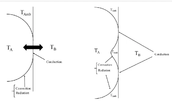
Figure 5.8: Contact between two bodies at different temperatures considering the different boundaries for each physical field. ... 105
Figure 5.9: Contact between two bodies at different temperatures considering the different boundaries for each physical field. ... 106
Figure 5.10: a) Example of a triangular linear mesh. ... 106
Figure 5.11: Example of an element with negative Jacobian. ... 107
Figure 5.14: Correction of the new boundary nodes. ... 110 Figure 5.15: Example of a boundary segments. ... 110 Figure 5.16: Cross product between a node that belong to a new mesh and the older element. ... 112 Figure 6.1: Mesh used to simulation for heat transfer validation a) linear triangle b) quadratic triangle c) linear quadrilateral d) quadratic quadrilateral. ... 116 Figure 6.2: Scheme to validate the prescribed temperature at the boundary of a cylinder. ... 116 Figure 6.3: Results for the analytical equation for the prescribed boundary temperature a)
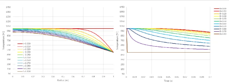
Temperature/Radius b) Temperature/Time evolution. ... 117 Figure 6.4: Results for Abaqus simulation for the prescribed boundary temperature a) Linear
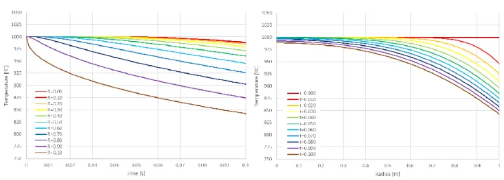
triangular elements b) Linear quadrilateral elements c) Quadratic triangular elements d) Quadratic quadrilateral elements. ... 118 Figure 6.5: Results for Empaktor software for the prescribed boundary a) Linear triangular elements b) Linear quadrilateral elements c) Quadratic triangular elements d) Quadratic quadrilateral elements. ... 119 Figure 6.6: Results for Empaktor software for the prescribed boundary temperature using only the diagonal values for the capacity matrix a) Linear triangular elements b) Linear quadrilateral elements c) Quadratic triangular elements d) Quadratic quadrilateral elements. ... 120 Figure 6.7: Results for Empaktor software for the prescribed boundary temperature using a pondered capacity matrix a) Linear triangular elements b) Linear quadrilateral elements c) Quadratic triangular elements d) Quadratic quadrilateral elements. ... 121 Figure 6.8: Scheme to validate the prescribed flux at the boundary cylinder. ... 121 Figure 6.9: Results for the analytical equation for the prescribed boundary flux a) Temperature/Time b) Temperature/Radius evolution. ... 122 Figure 6.10: Results for Abaqus simulation for the prescribed flux a) Linear triangular elements b) Linear quadrilateral elements c) Quadratic triangular elements d) Quadratic quadrilateral elements. ... 123 Figure 6.11: Results for Empaktor software for the prescribed Flux a) Linear triangular elements b) Linear quadrilateral elements c) Quadratic triangular elements d) Quadratic quadrilateral elements. ... 124 Figure 6.12: Results for Empaktor software for the prescribed flux using only the diagonal values for the capacity matrix a) Linear triangular elements b) Linear quadrilateral elements c) Quadratic triangular elements d) Quadratic quadrilateral elements. ... 125 Figure 6.13: Results for Empaktor software for the prescribed flux using a pondered capacity matrix a) Linear triangular elements b) Linear quadrilateral elements c) Quadratic triangular elements d) Quadratic triangular elements. ... 126 Figure 6.14: Mesh used for heat transfer validation for quadratic triangular and quadratic
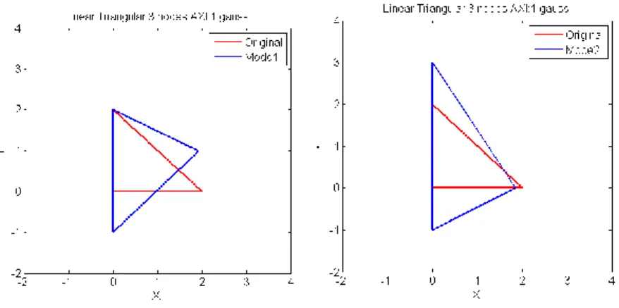
quadrilateral. ... 127 Figure 6.15: Results for prescribed temperatures a) Quadratic triangular elements in Abaqus b) Quadratic triangular elements Empaktor software c) Quadratic quadrilateral elements in Abaqus d) Quadratic quadrilateral elements Empaktor software. ... 128 Figure 6.16: Results for prescribed flux temperatures a) Quadratic triangular elements in Abaqus b) Quadratic triangular elements Empaktor software c) Quadratic quadrilateral elements in Abaqus d) Quadratic quadrilateral elements Empaktor software. ... 129 Figure 6.17: Axisymmetric deformation modes for the linear triangular element using 1 Gauss point. ... 131 Figure 6.18: Orthogonalizing deformation modes for the linear triangular element using 1 Gauss point. ... 131 Figure 6.19: Axisymmetric deformation modes for the linear triangular element using 1 Gauss point. ... 132 Figure 6.20: Axisymmetric deformation modes for the linear triangular element using 3 Gauss point. ... 132 Figure 6.21: Axisymmetric deformation modes for the linear triangular element using 7 Gauss point. ... 132
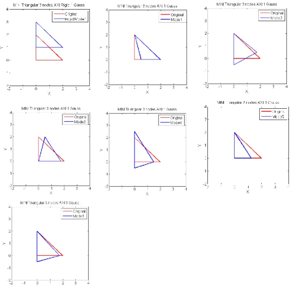
Figure 6.22: Axisymmetric deformation modes for the MINI linear triangular element using one Gauss point. ... 133 Figure 6.23: Orthogonalizing deformation modes for the MINI linear triangular element using 1 Gauss point. ... 133 Figure 6.24: Axisymmetric deformation modes for the MINI linear triangular element using one Gauss point. ... 134 Figure 6.25: Axisymmetric deformation modes for the MINI linear triangular element using three Gauss point. ... 134 Figure 6.26: Axisymmetric deformation modes for the MINI linear triangular element using three Gauss point. ... 135 Figure 6.27: Axisymmetric deformation modes for the MINI linear triangular element using seven Gauss point. ... 135 Figure 6.28: Axisymmetric deformation modes for the quadratic triangular element using one Gauss point. ... 136 Figure 6.29: Orthogonalizing deformation modes for the quadratic triangular element using one Gauss point. ... 136 Figure 6.30: Axisymmetric deformation modes for the quadratic triangular element using one Gauss point. ... 137 Figure 6.31: Axisymmetric deformation modes for the quadratic triangular element using three Gauss point. ... 138 Figure 6.32: Axisymmetric deformation modes for the quadratic triangular element using three Gauss point. ... 139 Figure 6.33 Axisymmetric deformation modes for the quadratic triangular element using seven Gauss point. ... 139 Figure 6.34 Axisymmetric deformation modes for the quadratic triangular element using seven Gauss point. ... 140 Figure 6.35: Axisymmetric displacement modes for the linear quadrilateral element using one Gauss point. ... 141 Figure 6.36: Orthogonalizing deformation modes for the linear quadrilateral element using one Gauss point. ... 142 Figure 6.37: Axisymmetric deformation modes for the linear quadrilateral element using one Gauss point. ... 142 Figure 6.38: Axisymmetric deformation modes for the linear quadrilateral element using 2x2 Gauss point. ... 143 Figure 6.39: Axisymmetric deformation modes for the linear quadrilateral element using 2x2 Gauss point. ... 143 Figure 6.40: Axisymmetric deformation modes for the linear quadrilateral element using 3x3 Gauss point. ... 143 Figure 6.41: Axisymmetric deformation modes for the linear quadrilateral element using 3x3 Gauss point. ... 144 Figure 6.42: Axisymmetric deformation modes for the quadratic quadrilateral element for one Gauss point ... 145 Figure 6.43: Orthogonalizing deformation modes for the quadratic quadrilateral element using one Gauss point. ... 145 Figure 6.44: Axisymmetric deformation modes for the quadratic quadrilateral element using one Gauss point. ... 147 Figure 6.45: Axisymmetric deformation modes for the quadratic quadrilateral element for 2x2 Gauss point. ... 148 Figure 6.46: Axisymmetric deformation modes for the quadratic quadrilateral element for 2x2 Gauss point. ... 149 Figure 6.47: Axisymmetric deformation modes for the quadratic quadrilateral element for 3x3 Gauss point. ... 150
Figure 6.48: Axisymmetric deformation modes for the quadratic quadrilateral element for 3x3 Gauss
point. ... 151
Figure 6.49: Axisymmetric deformation modes for the quadratic quadrilateral element for 4x4 Gauss point. ... 152
Figure 6.50: Scheme for the compression test. ... 153
Figure 6.51: Mesh used for compression test a) Linear triangular elements b) Quadratic triangular elements c) linear quadrilateral elements d) Quadratic quadrilateral elements. ... 153
Figure 6.52: Displacement results for the compression test for the different elements type. ... 154
Figure 6.53: Scheme to validate the prescribed temperature at the boundary cylinder. ... 155
Figure 6.54: a) Pressure teste for one linear quadrilateral element using two Gauss points to integrate the force b) using one Gauss point to integrate the force. ... 155
Figure 7.1: Layout of the preprocessor. ... 157
Figure 7.2: Option to model the simulation. ... 158
Figure 7.3: Software postprocessor overview. ... 159
Figure 7.4: Software postprocessor. ... 159
Figure 7.5: Software postprocessor thickness distribution. ... 160
Figure 7.6: Software core diagram. ... 161
Figure 7.7: Input file example. ... 163
Figure 7.8: Example of the results file. ... 163
Figure 7.9: Example of the update file. ... 164
Figure 7.10: Example of the list file. ... 165
Figure 8.1: Process selection for container height (cm). ... 167
Figure 8.2: Gob shape calculation. ... 167
Figure 8.3: Temperature distribution in gob loading for the case 1 for 0.334s, 0.342s, 0.427s and 0.763s. ... 175
Figure 8.4: Boundary temperature for gob loading stage for case 1. ... 175
Figure 8.5: Temperature distribution in gob loading for case 2 for 0.365s, 0.382s, 0.429s and 0.555s. ... 176
Figure 8.6: Boundary temperature for gob loading stage for case 2. ... 176
Figure 8.7: Displacement module in gob loading for case 2 for 0.368s, 0.375s and 0.381s. ... 177
Figure 8.8: Displacement module with the neckring detail in gob loading for case 2 for 0.3877s, 0.3973s 0.4165s. ... 178
Figure 8.9: Displacement vector with neck ring detail in gob loading for case 2 for 0.3877s, 0.3973s 0.4165s ... 178
Figure 8.10: Temperature distribution in gob loading for case 3 0.326s, 0.335s, 0.369s and 0.490s... 179
Figure 8.11: Boundary temperature for gob loading stage for case 3. ... 179
Figure 8.12: Temperature distribution in gob loading for case 4 for 0.255s, 0.310s, 0.373s and 0.772s. ... 180
Figure 8.13: Boundary temperature for gob loading stage for case 4. ... 180
Figure 8.14: Temperature distribution in gob loading for case 5 for 0.731s, 0.745s, 0.819s and 1.129s. ... 181
Figure 8.15: Boundary temperature for gob loading stage for case 5. ... 181
Figure 8.16: Temperature distribution in settle blow for the case 1 for 0.796s, 0.934s and 1.083s ... 183
Figure 8.17: Boundary temperature for settle blow stage for case 1. ... 183
Figure 8.18: Temperature distribution in settle blow for the case 2 for 0.555s, 0.666s and 1.333s. .... 184
Figure 8.19: Boundary temperature for settle blow stage for case 2. ... 184
Figure 8.20: Displacement module with the neckring detail in gob loading for case 2 for 0.555s, 0.744s 0.850s. ... 185
Figure 8.21: Displacement vector with the neckring detail in gob loading for case 2 for 0.555s, 0.744s 0.850s. ... 185
Figure 8.22: Temperature distribution in settle blow for the case 3 for 0.500s, 0.543s and 0.784s. .... 186
Figure 8.24: Temperature distribution in settle blow for the case 4 for 0.772s, 0.951s and 2.272s. .... 187
Figure 8.25: Boundary temperature for settle blow stage for case 4. ... 187
Figure 8.26: Temperature distribution in settle blow for the case 5 for 1.129s, 1.424s and 1.835s. .... 188
Figure 8.27: Boundary temperature for settle blow stage for case 5. ... 188
Figure 8.28: Temperature distribution in corkage reheat for the case 1 in 1.500s, for the case 2 in 2.044s, for the case 3 in 1.863s, for the case 4 in 4.090s and for the case 5 in 2.682s. ... 189
Figure 8.29: Temperature distribution in counter blow for the case 1 for 1.500s, 1.538s, 1.570s, 1.622s, ... 192
Figure 8.30: Simulation temperature of the boundary for counter blow stage for case 1. ... 192
Figure 8.31: Displacement module in counter blow for the case 1 for 1.500s, 1.538s, 1.570s, 1.622s, 194 Figure 8.32: Temperature distribution in counter blow for the case 2 for 2.044s, 2.161s, 2.376s, 2.571s, ... 196
Figure 8.33: Boundary temperature for counter blow stage for case 2. ... 196
Figure 8.34: Displacement module in counter blow for the case 2 for 2.044s, 2.161s, 2.376s, 2.571s, 198 Figure 8.35: Displacement vectors with the baffle detail in counter blow for the case 2 for 2.939s, 2.962s, 2.974s and 2.991s. ... 198
Figure 8.36: Temperature distribution in counter blow for the case 3 for 1.863s, 1.891s, 1.938s, 1.994s, ... 200
Figure 8.37: Boundary temperature for counter blow stage for case 3. ... 200
Figure 8.38: Temperature distribution in counter blow for the case 4 for 4.090s, 4.126s, 4.190s, 4.218s, ... 202
Figure 8.39: Boundary temperature for counter blow stage for case 4. ... 202
Figure 8.40: Temperature distribution in counter blow for the case 5 for 2.682s, 2.723s, 2.758s, 2.822s, ... 204
Figure 8.41: Boundary temperature for counter blow stage for case 5. ... 204
Figure 8.42: Temperature distribution in reheat for the case 1 in 3.958s, for the case 2 in 5.622s, for the case 3 in 4.705s, for the case 4 in 10.227s and for the case 5 in 6.117s. ... 205
Figure 8.43: Temperature distribution in invert for the case 1 in 4.514s , for the case 2 in 6.666s, for the case 3 in 5.490s, for the case 4 in 11.590s and for the case 5 in 6.823s. ... 207
Figure 8.44: Boundary temperature for invert stage for case 1, case 2, case 3, case 4 and case 5. ... 209
Figure 8.45: Temperature distribution in rundown for the case 1 in 4.514s, 5.201s, 5.833s. ... 210
Figure 8.46: Boundary temperature in rundown for case 1. ... 210
Figure 8.47: Temperature distribution in rundown for the case 2 in 6.666s, 7.222s and 9.111s. ... 211
Figure 8.48: Boundary temperature in rundown for case 2. ... 211
Figure 8.49: Displacement module in rundown for the case 2 in 6.666s, 7.222s and 9.111s. ... 212
Figure 8.50: Temperature distribution in rundown for the case 3 in 5.490s, 6.590s and 7.843s. ... 213
Figure 8.51: Boundary temperature in rundown for case 3. ... 213
Figure 8.52: Temperature distribution in rundown for the case 4 in 11.590s, 12.898s, 14.545s. ... 214
Figure 8.53: Boundary temperature in rundown for case 4. ... 214
Figure 8.54: Temperature distribution in rundown for the case 5 in 6.823s, 8.527s and 9.882s. ... 215
Figure 8.55: Boundary temperature in rundown for case 5. ... 215
Figure 8.56: Temperature distribution in final blow for the case 1 in 5.555s, 5.556s, 5.558s, ... 217
Figure 8.57: Temperature distribution in final blow for the case 2 in 9.111s, 9.125s, 9.133s, ... 218
Figure 8.58: Displacement module in final blow for the case 2 in 9.111s, 9.125s, 9133s, ... 219
Figure 8.59: Temperature distribution in final blow for the case 3 in 7.843s, 7.846s, 7.848s, ... 220
Figure 8.60: Temperature distribution in final blow for the case 4 in 14.545s, 14.552s, 14.563s, ... 221
Figure 8.61: Temperature distribution in rundown for the case 5 in 9.882s, 9.884s, 9.892s, ... 222
Figure 8.62: Temperature distribution in mould open for the case 1 in 7.292s, for the case 2 in 12.555s, for the case 3 in 10.294s, for the case 4 in 22.500s and for the case 5 in 14.282s. ... 223
Figure 8.63: Final boundary temperature for case 1, case 2, case 3, case 4 and case 5. ... 225
Figure 8.66 Bottle thickness (mm) distribution in case 3. ... 228
Figure 8.67: Final bottle shape for the case 4. ... 228
Figure 8.68: Bottle thickness (mm) distribution in case 4. ... 229
Figure 8.69: Bottle thickness (mm) distribution in case 5. ... 229
Figure 8.70: Temperature distribution in gob loading for the case 1 in 0.175s, 0.199s, 0.252s and 0.466s. ... 231
Figure 8.71: Boundary temperature for gob loading stage for case 1. ... 231
Figure 8.72: Temperature distribution in gob loading for the case 2 in 0.096s, 0.140s, 0.238s, 0.383s. ... 232
Figure 8.73: Boundary temperature for gob loading stage for case 2. ... 232
Figure 8.74: Temperature distribution in gob loading for the case 3 in 0.078s, 0.115s, 0.275s, 0.800s. ... 233
Figure 8.75: Boundary temperature for gob loading stage for case 3. ... 233
Figure 8.76: Temperature distribution in gob loading for the case 4 in 0.251s, 0.266s, 0.355s, 0.555s. ... 234
Figure 8.77: Boundary temperature for gob loading stage for case 4. ... 234
Figure 8.78: Displacement module in gob loading for the case 4 in 0.2513s, 0.2667s, 0.3213s ... 235
Figure 8.79: Displacement vector in gob loading for the case 4 in 0.2513s, 0.2667s, 0.3213s ... 235
Figure 8.80: Temperature distribution in gob loading for the case 5 in 0.088s, 0.107s, 0.421s, 0.625s. ... 236
Figure 8.81: Boundary temperature for gob loading stage for case 5. ... 236
Figure 8.82: Temperature distribution in gob loading for the case 6 in 0.076s, 0.128s, 0.303s and 0.460s. ... 237
Figure 8.83 Boundary temperature for gob loading stage for case 6. ... 237
Figure 8.84: Temperature distribution in gob loading for the case 7 in 0.497s, 0.531s, 0.635s, 0.820s. ... 238
Figure 8.85: Boundary temperature for gob loading stage for case 7. ... 238
Figure 8.86: Temperature distribution in gob loading for the case 8 in 0.095s, 0.548s, 0.609s, 0.676s. ... 239
Figure 8.87: Boundary temperature for gob loading stage for case 8. ... 239
Figure 8.88: Temperature distribution in baffle on for the case 1 in 0.800s, for the case 2 in 0.859s, for the case 3 in 1.147s, for the case 4 in 0.889s, for the case 5 in 0.972s, for the case 6 in 0.801s, for the case 7 in 0.957s and for the case 8 in 1.126s. ... 241
Figure 8.89: Temperature distribution in plunger up for the case 1 in 0.8000s, 0.8002s, 0.8003s ... 243
Figure 8.90: Boundary temperature in plunger up for case 1. ... 243
Figure 8.91: Temperature distribution in plunger up for the case 2 in 0.8588s, 0.8590s, 0.8592s ... 245
Figure 8.92 Boundary temperature for plunger up stage for case 2. ... 245
Figure 8.93: Temperature distribution in plunger up for the case 3 in 1.1466s, 1.1468s, 1.1469s ... 247
Figure 8.94 Boundary temperature for plunger up stage for case 3. ... 247
Figure 8.95: Temperature distribution in plunger up for the case 4 in 0.8888s, 0.8890s, 0.8891s ... 249
Figure 8.96 Boundary temperature for gob loading stage for case 4. ... 249
Figure 8.97: Displacement module in plunger up for the case 4 in 0.8888s, 0.8890s, 0.8891s ... 251
Figure 8.98: Displacement vectors in plunger up for the case 4 in 0.8888s, 0.8890s, 0.8891s ... 252
Figure 8.99: Temperature distribution in plunger up for the case 5 in 0.9722s, 0.9727s, 0.9729s ... 254
Figure 8.100 Boundary temperature for plunger up stage for case 5. ... 254
Figure 8.101: Temperature distribution in plunger up for the case 6 in 0.8013s, 0.8014s ... 256
Figure 8.102: Boundary temperature in plunger up for case 6 and the thickness (mm) in plunger up stage for case 6. ... 257
Figure 8.103: Temperature distribution in plunger up for the case 7 in 0.9572s, 0.9575s, 0.9580s ... 259
Figure 8.104 Boundary temperature for plunger up stage for case 7. ... 259
Figure 8.105: Temperature distribution in plunger up for the case 8 in 1.1267s, 1.1272s, 1.1277s ... 261
Figure 8.107: Temperature distribution in reheat for the case 1 in 2.733s, for the case 2 in 2.837s, for the case 3 in 3.160s, for the case 4 in 2.777s, for the case 5 in 2.847s, for the case 6 in 3.178s, for the
case 7 in 2.871s and for the case 8 in 3.943s. ... 263
Figure 8.108: Temperature distribution in invert for the case 1 in 3.760s, for the case 2 in 3.910s, for the case 3 in 3.733s, for the case 4 in 4.194s, for the case 5 in 3.819s and for the case 6 in 3.561s, for the case 7 in 3.487s and for the case 8 in 4.788s. ... 265
Figure 8.109: Boundary temperature for invert stage for case 1, case 2, case 3, case 4, case 5, case 6, case 7 and case 8. ... 267
Figure 8.110: Temperature distribution in rundown for the case 1 in 3.760s, 5.026s and 5.800s. ... 268
Figure 8.111 Boundary temperature for run down stage for case 1 ... 268
Figure 8.112: Temperature distribution in rundown for the case 2 in 3.910s, 4.627s and 4.907s. ... 269
Figure 8.113: Boundary temperature in rundown for case 2. ... 269
Figure 8.114: Temperature distribution in rundown for the case 3 in 3.733s, 4.543s and 5.467s. ... 270
Figure 8.115: Boundary temperature in rundown for case 3. ... 270
Figure 8.116: Temperature distribution in rundown for the case 4 in 4.194s, 4.974s and 5.972s. ... 271
Figure 8.117: Boundary temperature in rundown for case 4. ... 271
Figure 8.118: Displacement module in rundown for the case 4 in 4.194s, 4.974s and 5.972s... 272
Figure 8.119: Temperature distribution in rundown for the case 5 in 3.819s, 5.131s and 5.694s. ... 273
Figure 8.120: Boundary temperature in rundown for case 5. ... 273
Figure 8.121: Temperature distribution in rundown for the case 6 in 3.561s, 4.298s ... 274
Figure 8.122: Boundary temperature in rundown for case 6 and the thickness (mm) in run down stage for case 6. ... 275
Figure 8.123: Temperature distribution in rundown for the case 7 in 3.487s, 4.664s and 5.059s. ... 276
Figure 8.124: Boundary temperature in rundown for case 7. ... 276
Figure 8.125: Temperature distribution in rundown for the case 8 in 4.788s, 6.459s and 6.854s. ... 277
Figure 8.126: Boundary temperature in rundown for case 8. ... 277
Figure 8.127: Temperature distribution in final blow for the case 1 in 5.800s, 5.803s, 5.804s ... 279
Figure 8.128: Temperature distribution in final blow for the case 2 in 4.907s, 4.909s, 4.910s ... 280
Figure 8.129: Temperature distribution in final blow for the case 3 in 5.467s, 5.469s, 5.471s ... 281
Figure 8.130: Temperature distribution in final blow for the case 4 in 5.972s, 5.418s, 5.419s ... 282
Figure 8.131: Displacement module in final blow for the case 4 in 5.972s, 5.418s, 5.419s ... 283
Figure 8.132: Temperature distribution in final blow for the case 5 in 5.694s, 5.700s, 5.705s ... 284
Figure 8.133: Temperature distribution in final blow for the case 6 in 5.584s 5.583s... 286
Figure 8.134: Temperature distribution in final blow for the case 7 in 5.059s, 5.065s, 5.067s ... 287
Figure 8.135: Temperature distribution in final blow for the case 8 in 6.854s, 6.860s, 6.862s ... 288
Figure 8.136: Temperature distribution in mould open for the case 1 in 7.399s, for the case 2 in 8.205s, for the case 3 in 7.600s, for the case 4 in 7.750s, for the case 5 in 7.847s, for the case 6 in for the case 7 in 7.653s and for the case 8 in 10.516s. ... 290
Figure 8.137: Final boundary temperature for case 1, case 2, case 3, case 4, case 5, case 6, case 7 and case 8. ... 292
Figure 8.138: Bottle thickness (mm) distribution in case 1. ... 293
Figure 8.139: Bottle thickness (mm) distribution in case 2. ... 294
Figure 8.140: Bottle thickness (mm) distribution in case 3. ... 295
Figure 8.141: Bottle thickness (mm) distribution in case 4. ... 295
Figure 8.142: Real thickness (mm) distribution in case 4. ... 296
Figure 8.143: Thickness (mm) distribution in case 5. ... 296
Figure 8.144: Thickness (mm) distribution in case 6. ... 297
Figure 8.145: Thickness (mm) distribution in case 7. ... 298
Figure 8.146: Thickness (mm) distribution in case 8. ... 299
Figure 8.147: Volume evolution for blow and blow process for the case 1, case 2, case 3, case 4 and case 5. ... 301
Figure 8.148: Volume evolution for press and blow process for the case 1, case 2, case 3, case 4, case 5, case 6, case 7 and case 8. ... 303 Figure 8.149: Number of nodes for the case 1, case 2, case 3 case 4 and case 5. ... 304 Figure 8.150: Number of nodes for the case 1, case 2, case 3 case 4, case 5, case 6, case 7 and case 8. ... 305 Figure 8.151: Plunger displacement for case 1, case 2, case 3, case 4, case 5, case 6, case 7 and case 8 for a slip penalty value of 1.0e04. ... 307 Figure 8.152: Time increment for blow and blow process for case 1, case 2, case 3, case 4 and case 5. ... 309 Figure 8.153: Time increment for blow and blow process for case 1, case 2, case 3, case 4, case 5, case 6, case 7 and case 8. ... 311
List of Tables
Table 2.1: Viscosity reference temperatures. ... 11
Table 2.2: Composition of typical glass containers ... 18
Table 2.3: Oxides functions in glass containers. ... 19
Table 7.1: Files created during the simulation. ... 161
Table 8.1: Simulation cases for the blow and blow and press and blow process. ... 166
Table 8.2: Simulation variables for blow and blow (left) and press and blow (right) processes. ... 168
Table 8.3: Machining timing for the blow and blow cases being respectively the case 1, case 2, case 3, case 4 and case 5. ... 169
Table 8.4: Machining timing for the press and blow cases being respectively the case 1, case 2, case 3, case 4, case 5, case 6, case 7 and case 8. ... 171
Table 8.5: Air temperature considered in the different stages. ... 171
Table 8.6: Material chemical composition for different simulations cases in blow and blow and press and blow processes. ... 172
Table 8.7: Material behaviour for different simulations cases in blow and blow process. ... 172
Nomenclature
Physical Quantities
Symbol Description Unity [SI]
Scalar
A
Area [m2] 0, , , ,
A B C D T
Empirical constants iB
Biot number c Specific heat [JKg-1K-1] *c
Critical crack length [m]E
Young’s modulus [Pa]Fo
Fourier numberG
Shear modulush
Heat transfer coefficient [Wm-2K-1], , ,
x y zk k k k
Thermal conductivity [Wm-1K-1]L
Length [m] m Mass [Kg]p
Pressure [Pa]Q
Heat Energy [J]R
Molar gas constant [m2Kgs-2K-1mol-1]r Radius [m]
t
Time unity [s] 0t
Initial time [s]T
Temperature [K] 1,mT
,T
2,m Temperature mould node [K]i
T
Initial temperature [K] 𝑇𝑎, 𝑇∞ Ambient temperature [K] u Displacement [m]V
Volume [m3] cV
Characteristic volume [m3] Heat transfer coefficient [Wm-2K-1]
Penalty value
c
Heat transfer coefficient convection [Wm-2K-1]cr
heat transfer coefficient convection/radiation [Wm-2K-1]
Stefan–Boltzmann constant [Wm−2K−4]
Strain Rate [s-1] e
Elastic strain rate [s-1]p
Plastic strain rate [s-1]
Viscosity [Pa.s]0
pre-exponential factork
shear viscosity [Pa.s]
Penalty number
Density [Kgm-3]f
failure stress [Pa]e
Stress rate [Pa.s-1]G
Activation energy [J]L
Element size [m]T
Temperature difference [K]V
Volume difference [m3] Symbol Description Vectorb
Volume forces if
,f
applied forces iN
,N
Shape functionsR
Rotation matrix iQ
,Q
Thermal loads i T Nodal temperature iv
, v Velocity Symbol DescriptionB
Derivative matrixij
C
,C
Capacity matrixii
e
Dilatational strain rateij
e
Deviatoric strain rateij
K
,K
Stiffness matrixij
S
Deviatoric stress tensor𝛼𝑖𝑗 Thermal expansion tensor
𝜀𝑖𝑗 Strain tensor
ii
Dilatational strain tensorij
Strain rate tensorij
Stress tensor m
Dilatational stress Symbol Description Numberi
,m,n Matrix index Symbol Description Abbreviations VFT Vogel–Fulcher–Tammann equation AG Adam–Gibbs Equation WLF Williams-Landel-Ferry LawCPU Central Processing Unit
FEM Finite Element Method
RAM Random Access Memory
PLC Programmable Logic Controller
HEC Hot End Coating
CVD Chemical Vapour Deposition
CEC Cold End Coating
HTC Heat Transfer Coefficient
RI Reduced Integration
IS machine Individual Section Machine
C H A P T E R
1
1
Introduction
A brief introduction about the glass manufacturing is done in this chapter and, in addition, a thesis synopsis and the objectives are presented.
1.1 Historic Review of Glass Making
Created millions of years ago, glass is an abundant and easily accessible material that has been present since the formation of our planet. It is formed by high temperature phenomena such as volcanic eruptions, lightning strikes or by the impact of meteorites that melt the rock then, rapidly enough, solidifies it, making the liquid-like structure stay in a glassy state [1].
Lava spewed by volcanos gets cooled to form glass. Meteor impacts are also known to melt the earth’s crust and with the occurrence of subsequent impacts form smaller bits of glass [2]. Impactites are a natural occurring type of glass formed by amorphous crystalline material after the impact of a meteorite shockwave [2]. When glass was invented it was quickly noticed how resistant it was, how it didn’t suffer from devitrification as well as water corrosion. Our stone-age ancestors noticed the strength and sharpness of this material when they used obsidian to produce tools and arrowheads[1].
The melting of raw materials to create glass is a process that was discovered thousands of years ago. The Egyptians, no earlier than 7000 B.C., manufactured jewellery and glass beads [3]. In Mesopotamia, objects with coloured glazes containing copper compounds have been found dating to 4000 B.C. [2]. Feathery or zigzag patterns of coloured threads on the surface of some objects have also been found [4]. Glass was produced by the Egyptians until 1500 B.C. [3]. The recovered glass vessels from Egypt were manufactured between 14th and 16th century B.C. [2]. The adopted method is believed to have been to melt the glass, draw the threads out, turn them around a clay or sand object and then remelt the glass threads, using chemicals to give colour to the glass. Patterns were made by remelting pieces of coloured glass. The manufacture of Egyptian glass declined around the 11th century B.C. and in the meantime, it spread to other eastern Mediterranean regions such as Syria, Cyprus and Palestine. The major glass making centres became Syria and Palestine using the same techniques and colours that the Egyptians used, after 1000 B.C.
blowing technique the possibilities of shaping glass became endless [4]. Generating an amazing range of glass applications as well as improving the quality of glass jars and bottles making the glass drinking vessels popular [3]. The next step was to use clay moulds for contours while blowing the glass to create flasks and other shapes, they also realized that glass could be shaped freehand to any form they desired. This created decorative elements, handles, feet that could be added as one desired [4]. Around 400 B.C. Macedonia and Greece emerged also as centres of glass manufacture [2]. Techniques for making glass tableware such as bowls, the use of brilliant colours, also the use of lathes and grinding wheels to manufacture decorations had already been developed. Greeks developed a technique to sandwich gold layers between clear glass parts and the mosaic forming, this technique was developed in order to impart special colour effects. The Roman Empire, between 3rd and 2nd century B.C., spread the making of glass through Rome and Italy with the methods of imparting different colours and glass blowing becoming widely popular. The making of cameo glass became one of the most sought techniques of this era [2]. Romans became the first civilization to experiment blowing glass inside moulds leading to improve the glass jars and bottles and the production of drinking vessels thereafter [5]. After the Roman Empire, the Byzantine regions (Greek Empire), under Islam, came with new developments. In the 7th century A.C. glass manufacture thrived in Syria and Palestine. The hedwig glass belongs to this era and it was created using diamond cutting. Baghdad emerged as the glass making centre of the 9th A.D. century after the Arab invasion that spread through most part of Asia and the closest Mediterranean parts of Europe. In the 13th century A.C. and through the next two centuries Persia became the major manufacturer of fine glassware and developed the technique of grinding glass surfaces. In the 14th century the independent republic of Venice became the centre for glass manufacture of Europe. Two significant developments occurred at this time: the discovery that the addition of calcia gave bright, shiny glass and the glass could also be worked to be incredibly thin, crystal-like clear with feather-light weight; the second was the creation of ice glass by plunging molten hot glass into ice cold water with an iron pipe for just a few moments and then blown, creating what appeared to be a tiny cracks within its surface. Glass making only flourished to the other parts of Europe by the end of the 16th century, it was at this time that English workers develop the waldglass (green or amber tinted glass). Development in Europe came in the form of techniques and popular designs that made glass articles affordable by the middle classes. With the 19th century came the birth of the mechanized glasswork not only in Europe but the United States as well. Opaline, a translucent milky-white glass, was created in France around 1810 by adding metallic oxides to the glass mixture. The modern method of glass making grew roots in most countries in Europe, America, Japan, India and China in the end of the 19th century. It was in the 20th century that glass became part of the human life with an evolution of manufacturing techniques and a deeper scientific understanding of it. This scientific understanding of glass was proportionally connected to the growth of chemistry and physics understanding, mainly in the field of inorganic materials. This growth was born from the observation of the effects of the addition of oxides and other chemicals produced in silica glass [2]. The invention of glass vacuum tubes paved the path to create most modern electronics today. The development of glass fibre optics is revolutionizing the telecommunications industry by replacing copper wires enhancing our ability to transmit data around the world [3]. Since its discovery glass became a stalwart material for our society, from its commonly day uses to architecture, to science and many other fields.
1.2 History of Glass Moulding
Blow moulding is believed to have been created around 1821 in Bristol, England. In 1859 Mein of Glasgow designed the first vertically spilt iron mould which had a movable base plate to make bottles by blowing compressed air. The biggest change to the manual process was to make the mouth or finish first so that the glass could be held in place while the rest of the manufacture operations were performed [6]. In 1866, H.M. Ashley and Josiah Arnall changed the way to fabricate containers. To answer the demands for sterile and refrigeration containers they created a new way to produce bottles, with semi-automatic machines, using an inverted mould with a plug at the bottom to create the mouth. [6]. While in hand blowing, the bottle neck was finished last (after blowing operations), a major change happened when this operation was made first by the machine [1]. In 1887, Ashley made some improvements, a separate parison1 mould gave a better
distribution of wall thickness and a separate neckring mould to hold glass while being manipulated. This was done with a simple machine that needed to be fed gobs of glass by hand, reducing the labour cost or so it was claimed. This achieved an almost consistent weight of glass and internal capacity [6].
In the 1900 the progressive use of soda-lime-silica glass was started in the glass containers production. Mechanization in the production of glass containers was also in development.
An American engineer called Michael Owens (1859–1923) invented an automatic bottle blowing machine. This innovation was a successful process, which arrived in Europe after the turn of the century and considerably transformed the containers industry. A further improvement of the process is given by Hartford Company which invented the feeder in 1922 to provide the forming machines with a thermally conditioned glass gob2. The feeder mechanism worked constantly as an extrusion machine which create a
uniformly gob with a specified rate.
The feeders are still employed todays and with the invention of individual section (IS) machines by 1925, they deliver several forming machines. A great advantage of the machine was that one section could be shut down to change moulds without stopping the production in the other sections. These inventions answered the growing demand for glass containers.
Along time glass as become a common material used in diverse applications. Firstly, empirical knowledge had a principal importance in developing glass industry. Nowadays trial and error is still a manner to improve quality in glass industry, however this type of production is highly time consuming and expensive. We live in a world in which glasses play a very important role in all aspects of our daily life and this is enough reason for us to study its forming processes.
1.3 Glass Containers Industry
Glass forming processes take place at high production rates. At the same time, glass manufacturers desire to optimize glass products to their customer’s satisfaction. Glass containers process is a very complex procedure which must be thoroughly controlled in order to be able to satisfy the even more exigent costumers. Unfortunately, practical experiments are in general quite expensive, whereas the majority has to be performed under complicated circumstances. In addition, each glass manufacturing company keeps secret about its own experimental data. Therefore, it is no surprise that in the recent past glass process techniques were based on experience, rather than on scientific research. Nowadays computer simulation models are necessary to gain improvement and a better understanding of glass forming processes.
The glass containers manufacturers have to deal with challenges to improve the productivity of the plant or reduce the productions costs without the decrement of the quality levels imposed by the customer. Glass industry needs to work 24h per day and 7 days a week in order to keep the furnace working. Combine high productivities and low production costs are the main goals that the glass industry tries to achieve. Glass industries require sustainable profitability, quality and increase market share in the packaging industry. To maintain the glass containers quality the forming process needs stability. Glass industry tends to approve the new technologies slowly preferring to use the empirical knowledge of their workers. The competitiveness in glass industry brings the necessity to improve the design and the quality of their products. Different shapes, glass composition, colours may needs different changes in the processing parameters which can have very expensive costs.
Nowadays, glass industry has achieved considerable goals in efficiency and production rate without loss of product quality. They have been doing progresses in developing raw materials and processes using the knowledge created along the years. Utilizing the knowledge existent in materials properties and tools and R&D progress and opportunities, the glass industry is improving the production. Glass researchers are
making progress in manufacturing new functional glasses, upgrading existent technology continuously and also the simulation of the process can play an important role in this field.
1.4 Glass Container Quality
Glass has a wide range of uses. The main characteristics of glass are including shock-resistance, soundproofing, transparency and reflecting properties, which makes it particularly suitable for a wide range of applications, such as windows, television screens, bottles, drinking glasses, lenses, fibre optic cables, sound barriers and many other applications.
Glass products are engineered to fit the needs of customers, the major qualities their claim are resistance, durability, and ability to support rigorous condition. Special customers may need especial glass with special chemical composition and the glass industry should be prepared for the melting point and especial production processes needed to meet these requirements.
A key issue in glass containers is the wall thickness distribution. The thicker the container, the stronger it is and the less easily it breaks. The thinner the container, the lighter it is and less costs are spent on material. The optimal wall thickness distribution have to be optimize between these aspects. The ideal thickness distribution is not necessarily uniform, as some parts of the container are more vital than others, e.g. corners, and should be thicker for optimal strength. The difficulty in blow moulding a container with a prescribed wall thickness distribution is that the corresponding initial operating settings are not known beforehand. There are essentially two ways to deal with this. The first approach is the use of numerical simulation. If the initial operating conditions can be estimated, for example by empirical expertise of the process, a mathematical model can be developed that can directly compute the corresponding container production. Then, the initial operating settings of the blow moulding process can be adjusted to improve the wall thickness of the computed container. The first approach to attempt the desired wall thickness distribution is commonly a trial and error procedure, which is often based on the manufacturer’s knowledge of the process. However, empirical expertise is often insufficient to find the initial operating settings, particularly when innovative processes are involved. A second approach is to solve an inverse mathematical problem to find the initial operating settings corresponding to the container with the desired wall thickness distribution. This class of inverse problems is quite challenging, as in general couple, highly nonlinear physical systems and complicated geometries are involved [7]. Usually, numerical optimization methods are employed to find a solution to the inverse problem [8]. Some advantages of lighter weight containers are, less cost to manufacture, higher forming machine production rates possible, shipping load and space requirements reduced, more competitive with plastic, cans, and paper containers.
The design of a container must be suitable for weight reduction without a reduction in strength. This is extremely important because a bottle can usually be effectively made lighter in weight only if can be designed with a stronger structural shape taking into consideration the particular forming process used to produce the containers.
Light weighting is important to improve productivity, when the glass containers are thinner and lighter some contribution for productivity are made and are the following,
o Lighter weight containers means that more containers per ton of glass can be produced.
o Lighter weight means less glass and therefore, less heat to be removed and the result is an increase in production speed.
o Saving weight also reduces glass cost per container which is a contribution of financial productivity.
Glass is basically made from sand and sand is largely spread throughout the earth’s crust with very high purity of silica and uniform grain size. Uniform grain size is a very desirable quality because it can correspond to a consistent chemical composition. Sand before being used as a raw material needs some treatments to remove impurities like iron and ferric oxide, chromic oxide and heavy minerals. In the glass
the control of chemical composition of raw materials used in the processes is necessary in order to guarantee a high and constant level of quality of the product.
Glass is chemically inert, and environmentally friendly. Glass material is a preferred material of choice for the packaging industry worldwide for many years. The knowledge of the temperature is important in almost all stages of the glass production and glass processing. During the melting process in the glass tank the temperature influences the homogeneity of the glass melt. Undesired cracks could be the result of a wrong cooling of the glass [9]. Thus, the knowledge of the right temperature is important to guarantee the quality of the final products.
Heat conduction, heat convection and radiation plays an important role in the production of glass containers. Other properties, such as viscosity, thermal expansion, and electrical conductivity, are strongly dependent on glass composition. Glass is a very versatile material, it is quick to form in shape, cheap to produce and, depending on the recipe used it can be extremely durable. It can be transparent, opaque and take a greater range of colour and decorative effects than any other man made material.
Viscosity is the most important mechanical property in glass material and varies enormously with chemical composition. Since viscosity varies with chemical composition and is highly dependent of temperature, different glass types have very different behaviours while are worked at high temperatures.
Customers usually take no particular interest in the chemical composition of glass. Most catalogues by glass producers, therefore, do not indicate the chemical composition of the products. For glass producers, however, the chemical composition of the products and its control are highly important. To know the temperature dependence on viscosity is of fundamental importance for glass science and technology [10].
1.5 Glass Container Simulation
Modelling has become an important tool to accelerate the innovation while reducing the trial and error methods commonly used in production environments. Numerical simulation provides detailed information about forming process and thereby helps in determining the effects of different parameters on the final form of the item. Simulation can be done in shorter times and their costs are much lower than that of making trial moulds. Therefore, numerical simulation technique has the potential capacity to largely replace the other design techniques.
Glass forming techniques are still mostly based on empirical knowledge and hands on experience. Experimental trial using glass forming machines are in general very expensive and time consuming. Simulations give an alternative to an empirical knowledge avoiding the trial error procedures used in factories. Also help to reduce waste as well as the wall thickness reducing weight and maximizing strength.
In the last years, simulations software based on the finite element method has become an important tool to improve understanding, controlling and optimized the process. It is expected that this can give the final shape, thickness distribution, temperature distribution, etc.
The production of glass container takes place at high production rates. Time quality factors of the products, such as smoothness, strength, weight and cooling conditions, are optimized in order to pass the quality control process. To optimize and control the process is required knowledge. Unfortunately, measurements are often complicated, considering that blow moulding processes take place at high rates in closed constructions under complicated circumstances at high temperatures. Simulation models may offer a good alternative for complicated experimental measurements.
Glass-packaged products face a significant competitive pressure from products made of alternative materials. Nowadays, plastic, paper and related material and metallic (Aluminium and steel) containers share a large part of the container market. This has forced the glass industry to produce lighter containers (this has pushed the tools toward and the glass containers have more uniform glass distribution all over the article) for short-term conservation purposes while offering new attractive designs and promoting glass
![Figure 2.1: a) Examples of a cord defects after cooling. b) Glass cord observed by viewing in polarized light [12]](https://thumb-eu.123doks.com/thumbv2/123dok_br/15588483.1050292/33.892.199.712.95.411/figure-examples-defects-cooling-glass-observed-viewing-polarized.webp)
![Figure 3.47: a) Gob loading b) Settle blow c) Counter blow d) Invert e) Final blow f) Take out [12]](https://thumb-eu.123doks.com/thumbv2/123dok_br/15588483.1050292/75.892.125.781.393.1071/figure-gob-loading-settle-blow-counter-invert-final.webp)
![Figure 3.48: a) Gob loading b) Baffle on c) Plunger up d) Invert e) Rundown f) Final Blow g) Take out [12]](https://thumb-eu.123doks.com/thumbv2/123dok_br/15588483.1050292/78.892.268.766.82.415/figure-loading-baffle-plunger-invert-rundown-final-blow.webp)