The Zero Lower Bound on nominal interest rates and its impact on monetary policy in the “New Normal”

(1)

The Zero Lower Bound on Nominal Interest

Rates and Its Impact on Monetary Policy in

the “New Normal”

Daniel Bäumler

Dissertation written under the supervision of Professor Nuno Alves

Dissertation submitted in partial fulfilment of requirements for the MSc in

Economics, at the Universidade Católica Portuguesa and the Université

(2)

The Zero Lower Bound on Nominal Interest Rates and Its Impact on

Monetary Policy in the “New Normal”

Daniel Bäumler1

Universidade Católica Portuguesa & Université Catholique de Louvain

Supervisor: Nuno Alves

Universidade Católica Portuguesa & Banco de Portugal

Abstract

This dissertation aims to illustrate the impact of the Zero Lower Bound (ZLB) on nominal interest rates, based on a deterministic simulation of Fernández-Villaverde and Rubio-Ramírez’ (2006) DSGE model of the U.S. economy. I calibrate the model for 2 different steady states, the first based on historical data (old steady state) and the second matching the most recent data, with lower inflation and lower real interest rates (new steady state). Within these calibrations I simulate the impact of a set of representative shocks. The ZLB appears to be of minor relevance in the old steady state while it is found to be a significant constraint in the new steady state. The associated impact on activity is relatively small but not negligible. My results are robust assuming alternative monetary policy rules. Hence, I conclude that conventional monetary policy tools are insufficient to anticipate the increased risk of hitting the ZLB in the new steady state. Further analysis of the exact transmission mechanism is warranted due to the simplified assumptions underlying this

dissertation.

Sumário

Esta dissertação pretende ilustrar o impacto do limiar inferior das taxas de juros nominais (ZLB), com base numa simulação determinística do modelo DSGE para os EUA apresentado em Fernández-Villaverde e Rubio-Ramírez (2006). O modelo é calibrado para 2 estados estacionários, o primeiro com base em dados históricos (antigo estado estacionário) e o segundo com base em dados recentes,

caracterizados por uma menor inflação e taxas de juros reais mais baixas (novo estado estacionário). Com base nesta calibrações, é simulado o impacto de um conjunto de choques representativos. O ZLB parece ser de menor relevância no antigo estado estacionário enquanto se verifica ser uma restrição significativa no novo estado estacionário. O impacto associado na atividade é relativamente pequeno, mas não negligenciável. Os resultados são robustos a regras de política monetária alternativas. Assim, concluo que os instrumentos convencionais de política monetária são insuficientes para evitar o maior risco de atingir o ZLB no novo estado estacionário. Mais investigação sobre o mecanismo de transmissão monetária próximo do ZLB é necessário, dadas as hipóteses simplificadoras subjacentes a esta dissertação.

Email address: [email protected] / [email protected]

1_{I am thankful to Professor Nuno Alves for all the advice and guidance during the last year, in particular during}

the process of writing this dissertation. I would also like to thank Professor Teresa Lloyd Braga and Mme Géraldine Carette for their help and suggestions throughout the Master’s. Finally, I am grateful to my parents and friends, for their patience and support I have always had.

(3)

1 Introduction

The Federal Reserve Board decision to raise its target interest rate in December 2015

followed an extended period of more than 7 years where interest rates were stuck at the zero lower bound (ZLB). Not only did this occur in the U.S. but also in several other advanced economies was the ZLB constraint on nominal interest rates binding for an extended period of time (see Annex A and Dordal-i-Carreras, Coibion, Gorodnichenko & Wieland, 2016).

Obviously the sharp drop in interest rates across the world was first and foremost a reaction to the Great Recession of 2009. However, the extended duration of rates staying at historically low levels gives reason to believe that a more fundamental and persistent development

occurred. Most prominently, Summers (2014b) argues that the equilibrium real rate of interest has decreased permanently over the last years. This is also related with the concept of secular stagnation which among other things implies that potential output growth has decreased permanently (Teulings & Baldwin, 2014). Other authors have focused on the evolution of the natural rate of interest (Williams, 2003) which has decreased likewise, alongside nominal rates of interest and inflation rates.

This dissertation aims to analyze the impact of the ZLB constraint on nominal interest rates in this “new normal” – characterized by lower potential output growth, lower trend inflation, and a lower natural rate of interest2_{. In particular I will try to answer two questions: i) “Does the}

ZLB constraint change the dynamics of an economy following a set of shocks?”; and ii) “How do the features of the ‘new normal’ constrain the monetary policy response given the ZLB constraint?”. This will be done by simulating a dynamic stochastic general equilibrium (DSGE) model of the U.S. economy by Fernández-Villaverde and Rubio-Ramírez (2006) in a deterministic setting with perfect foresight and fully rational agents. This dissertation is structured as follows. After motivating the choice of this topic by presenting further data and reviewing the literature (section 2), the basic model set-up and its steady state will be

presented (section 3). The model calibration follows in section 4. Afterwards the interaction of the model with the ZLB will be explored in detail, first, under a set of illustrative shocks, then, by a set of representative shocks based on historic data (section 5). A brief sensitivity analysis serves to support the results in section 6. The dissertation concludes with a summary

2_{This dissertation follows William’s (2015) more long-run oriented definition of the natural rate of interest. This}

concept refers to the real policy rate which is consistent with the economy running at its full potential assuming transitory shocks have subsided which is expected to prevail only over a time-horizon of about 5 to 10 years.

(5)

of the most important results and a brief review of mitigating strategies with respect to the increased risks of hitting the ZLB.

2 Motivation

This dissertation is not only motivated by recent literature but especially by macroeconomic evidence. Looking at the data, the secular stagnation hypothesis seems, so far, to be

confirmed. Holston, Laubach, and Williams (2016) estimated the inflation-adjusted natural rate of interest for the U.S., Canada, the U.K., and the euro area as displayed in figure 1. While it was in a range of around 2.5% to 3.5% in 1990, it decreased over the years, and reached a range of around -0.5% to 1.5% in 2015.

Figure 1. Estimated inflation-adjusted natural rates of interest for Canada, the euro area, the U.S. and the U.K..

Figure adopted from Holston, Laubach & Williams (2016).

Accordingly, a similar decline in trend growth can be observed. In the euro area it dropped from slightly below 3% during the 1980s to slightly above 1% in recent years (figure 2) whereas in the U.S. it declined from about 3.5% to 1.5% over the same time span (figure 3).

(6)

Figure 2. Euro area natural rate of interest and trend growth. Blue stripes represent periods of recession and r*

stands for the natural rate of interest. Figure adopted from Holston, Laubach & Williams (2016).

Figure 3. U.S. natural rate of interest and trend growth. Blue stripes represent periods of recession and r* stands

for the natural rate of interest. Figure adopted from Holston, Laubach & Williams (2016).

Furthermore, inflation rates have most recently decreased to historically low levels too. For instance, in the euro area, inflation has been below the target rate of 2% for more than 3 years, fluctuating around zero for almost 2 years (ECB, 2016). Also the U.S. has experienced a recent, but meanwhile 2-to-3-years-lasting, drop in inflation rates to levels close to zero (FRED, 2016). Also, supporting the argument of secular stagnation, it can be underlined that

(7)

projections of key parameters, such as potential output growth or the natural rate of interest, have been continuously and repeatedly revised downwards by the Federal Reserve Board since 2012 (Bernanke, 2016). While the natural rate of interest was seen at 4.25% and potential output growth at 2.3% to 2.5% in 2012 they were projected to be only 3.0% respectively 1.8% to 2.0% in 2016. Bernanke (2012) interprets these revisions as an acknowledgement by the FED of the new economic reality we live in.

This brings me to the next observation one can take from reviewing recent literature on the natural rate of interest and output growth potential. Considering characteristics of the data of the last few years, researchers investigated intensively on what the “new economic reality” or the “new normal” actually is. Various research confirms the secular stagnation proponent’s hypothesis of these developments to be non-transient (Hamilton, Harris, Hatzius & West, 2015; Lubik & Matthes, 2015; Williams, 2015). Laubach and Williams (2003), for instance, developed a model which is geared towards measuring highly persistent movements in the natural rate of interest. Their application of this model with most recent data does indeed detect a persistent decline of natural interest rates to levels close to zero which can be ascribed to a large part to the decrease in trend output growth (Laubach & Williams, 2016). Output growth for the U.S. is estimated to be at about 1.6% over the next 10 years according to Fernald’s (2016) forecasts. Meanwhile, he expects U.S. GDP per capita to grow by less than 1% per year.

The reasons for the adjustment of this “new normal” have been subjected to further research and go beyond Laubach and William’s (2016) conclusions. Part of the underlying reasons for these developments may be in fact structural, long-term developments. Another part,

however, can be ascribed to the long-lasting effects caused by the Great Recession which is referred to as hysteresis (Summers, 2014a). To be more precise, hysteresis is the theory that explains how a severe economic shock can have adverse effects on potential output, as the structure of the economy is impacted sustainably by this shock (in my case, this would be the Great Recession). Another theory argues that the more fundamental reasons for the observed secular stagnation is the reversal of total factor productivity (TFP) growth to its historical norm (Gordon, 2014). According to Gordon (2014) this is complemented with a set of structural headwinds: demographics change towards an aging and stagnant population which has higher savings needs; the average (U.S.) education level is not likely to further increase significantly; the wealth distribution became more unequal slowing down the middle class income growth; and public debt might have reached levels at which current deficits become

(8)

unsustainable. All these developments cause a shift in the global supply of and demand for save assets, creating a global savings glut (Summers, 2014b; Williams 2016) which in turn impacts the real rate of interest.

Obviously, these structural and persistent changes in economic conditions triggered a large set of research on the related consequences. The ZLB used to be considered to have a minor relevance for monetary policy, under the structural conditions prevailing in the late 1990s and early 2000s (Coenen, Orphanides & Wieland, 2003). Hitting the ZLB was believed to be a very rare, infrequent event which would only occur if nominal interest rates fell very

significantly below their target level (Schmidt-Grohe & Uribe, 2010). The likelihood of ZLB events was often estimated to be in the area of approximately 1% to 5% (Dordal-i-Carreras et al., 2016). In contrast, under the current structural features characterizing advanced

economies, the ZLB constraint on nominal interest rates is more likely to become binding. In this case, the room for stimulating policy rates gets smaller, and hence, unconventional monetary policy tools gain in relevance. Considering new cross-country time series, Chung, Laforte, Reifschneider and Williams (2012) for instance, suggest that the likelihood of hitting the ZLB vis-à-vis models calibrated based on pre-2010 figures has doubled. Recessions are expected to be longer lasting and more severe, recoveries to be slower, inflation rates to be more likely very low (Reifschneider & Williams, 2000; Williams 2016). ZLB events are generally more persistent and costlier than previously thought. Williams (2009) for example, estimates the cost of a 4-year ZLB event to amount up to $1.8 trillion. That is related to the fact that potential cost of such an event rise disproportionally with its duration. One long ZLB episode is thus costlier than two short ones with the same cumulative length (Coibion,

Gorodnichenko & Wieland, 2012).

In this thesis, I will illustrate the impact of some of these issues based on a standard DSGE model with an explicit ZLB constraint on nominal interest rates. The main features of the model are presented in the next section.

3 Model Set-Up

The model used for the analysis is the baseline sticky prices-sticky wages model presented in Fernández-Villaverde and Rubio-Ramírez (2006). There are four sectors in this economy: households, final good producers, intermediate good producers, and the monetary authority. Agents behave fully rationally and have perfect foresight.

(9)

3.1 Deterministic Model Set-Up

This dissertation relies on simulating a deterministic version of the original model, which is the more appropriate approach considering that I do not want to linearize the model around a steady state and that the focus of the analysis will be comparing two different economic regimes, characterized by different steady states (Griffoli, 2013). As described in sections 1 and 2, several key economic parameters have shifted to new levels and this shift will be analyzed in the simulations. Furthermore, the shocks which will be applied to the model are relatively large which makes a deterministic set-up more appropriate too. Besides, there is no perfect way (yet) of dealing with a non-linear, stochastic model analytically. Hence, working with a deterministic set-up serves the illustrative goals of this dissertation better, as it allows to work in a more transparent and simpler setting. In the following the most important characteristics of the model are summarized. For a full representation of this model please refer to Fernández-Villaverde and Rubio-Ramírez’ (2006) original paper or Annex B and C of this dissertation which contain a more comprehensive summary of this model, respectively the deterministic steady state equations.

3.2 Model Agents

There is a continuum of households which maximizes lifetime utility which is a function of consumption, real money balances and hours worked, subject to an intertemporal budget constraint. Households have habit persistence and supply labor according to a Frisch labor supply elasticity. An intertemporal preference shock as well as a labor supply shock enter the households’ utility function, which both follow first-order autoregressive processes (AR(1)). These processes have been modified in such a way that the shocks follow a fully deterministic path.

As households supply labor to the intermediate goods producer they set their wages according to Calvo’s setting which implies that only a fraction of all households can modify their wage in a given period while the remaining households can only index their wage by past inflation. Besides spending it on consumption households can also save and invest their income. Investment and an investment-specific technology shock, which also follows an AR(1) process, determine capital evolution.

Having access to technology and renting cost-optimal combinations of capital and labor, a continuum of intermediate goods is produced and sold to final good producers. The

intermediate good producers’ production can be described as a function of capital, labor, and

(10)

deterministic shock to neutral technology and the investment-specific technology shock. Intermediate goods producers also set their prices according to Calvo’s scheme which implies that only a fraction of them can change their prices in a given period whereas the remaining firms can only index their prices by past inflation.

In the perfectly competitive sector of final good production, profit maximizing firms, taking all prices as given, use a set of intermediate goods, which are characterized by a given elasticity of substitution, to produce one final good.

The monetary authority steers the nominal interest rate according to the following Taylor rule,

𝑅_𝑡 𝑅 = ( 𝑅_𝑡−1 𝑅 ) 𝛾𝑅 ( (Π𝑡 Π) 𝛾Π ( 𝑦_𝑡𝑑 𝑦_𝑡−1𝑑 Λ_𝑦𝑑 ) 𝛾𝑦 ) 1−𝛾𝑅 𝑒𝑚𝑡 (1),

in which 𝑅𝑡 represents the nominal gross interest rate, 𝑅 the steady state nominal gross

interest rate, Π𝑡 the rate of inflation, Π the target or steady state rate of inflation, 𝑦𝑡𝑑 𝑦_𝑡−1𝑑 real

output growth, Λ_𝑦𝑑 the steady state rate of output growth, and 𝑚_𝑡 a (deterministic) monetary

policy shock. Monetary policy is executed through open market operations which are financed by lump-sum transfers, 𝑇𝑡.

There are different methods of implementing the ZLB, especially relevant in a stochastic context3_{. Since the subsequent simulations will be run in a deterministic environment, the}

ZLB constraint can be simply enforced as described below in equation (2). Straightforwardly, monetary policy follows a rule whereby interest rates will be zero if the reaction function would prescribe negative interest rates.

𝑅_𝑡= 𝑚𝑎𝑥 { 𝑅 (𝑅𝑡−1 𝑅 ) 𝛾𝑅 ( (Π𝑡 Π) 𝛾Π ( 𝑦_𝑡𝑑 𝑦_𝑡−1𝑑 Λ_𝑦𝑑 ) 𝛾𝑦 ) 1−𝛾𝑅 𝑒𝑚𝑡_{; 0} } (2).

3_{One alternative is to do a log-linear approximation ignoring the ZLB, and only applying the constraint ex-post}

(Eggertsson & Woodford, 2003). However, this approach would violate the rational-expectations- respectively the perfect-foresight-assumption. Hence, a more appropriate alternative is to solve the model nonlinearly. Fernández-Villaverde et al. (2015), for instance, derive conditions involving expectations in order to smoothen the Taylor rule’s kink at the ZLB. Thus, the nominal interest rate can be calculated without any approximation.

(11)

4 Model Calibration

The original calibration presented in Fernández-Villaverde (2010), which is based on historical data, will be the basis for the steady state associated with the “old regime”, prevailing until the early 2000s. The “new normal”, or as I will call it throughout this

dissertation, the “new regime”, will refer to the current economic conditions, characterized by lower real rates, lower potential output growth and lower inflation rates.

Fernández-Villaverde (2010) provides a full calibration of their model for the U.S. economy which is, for the most part, being adopted for the subsequent simulations within the “old regime”. The discount factor, 𝛽, is estimated to be 0.998 which is rather high compared to more standard choices of around 0.994 (Fernández-Villaverde et al., 2012). Habit persistence,

h, is estimated to be 0.97 which can also be considered a comparatively high value. This is

important though as it yields a model that responds to shocks slowly. The inverse of the Frisch elasticity of labor supply, 𝛾, is 1.17. That is relatively high, and hence, close to values suggested by microeconomic literature. On the other hand, a disadvantage of a low Frisch elasticity is that preference shocks need to be rather large to trigger an appropriate model response (Fernández-Villaverde, 2010). The Calvo parameters for price- respectively wage-adjustment are specified to be 0.82 respectively 0.68. This ensures nominal rigidities in this model. The price-adjustment parameter implies that an average pricing cycle lasts 5 quarters whereas the wage-adjustment parameter ensures an average of 3 quarters per wage cycle. The Taylor rule is specified such that the Taylor principle is being respected with a coefficient on inflation of 1.29. The coefficient on output is 0.19 which is rather small and implies a weak response of monetary policy to output gaps. A relatively big coefficient on lagged interest rates of 0.77 signals that monetary policy follows a smooth path and does not react abruptly to shocks. The estimated target, respectively steady state rate of inflation, Π, is 4% annually, which is appropriate, considering historic data. When specifying the “new regime” the steady state rate of inflation shall be 2% to incorporate actual inflation targets and

decreased inflation expectations.

Steady state neutral technology growth, Λ𝐴, and steady state investment specific technology

growth, Λ𝜇, are originally estimated to ensure an overall, annual steady state output growth,

Λ_𝑦𝑑, of 1.8% which is in line with the average historic real per capita growth rate of 1.8% for

the U.S. between 1970 and 20164_{. Nevertheless, these parameters are maintained for the “old}

(12)

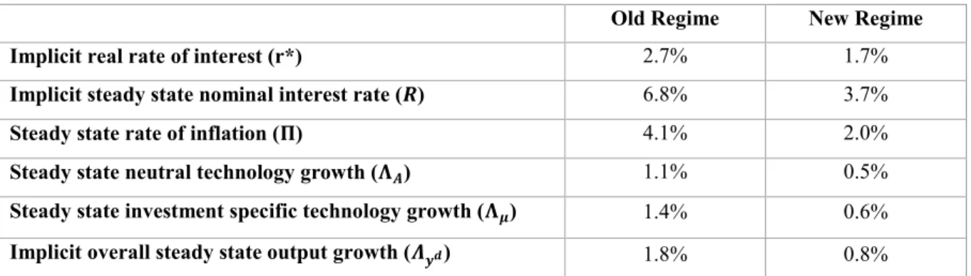
regime”. In order to anticipate the hypothesized lower output growth potential, they are specified to trigger an overall output growth of 0.8% under the “new regime” which represents a one-percentage-point-drop – twice the reduction in FED projections between 2012 and 2016 (Bernanke, 2016). Considering the historical U.S. output growth rate of 2.8% and Fernald’s (2016) projection of 1.6% annual U.S. output growth for the next 10 years from today, a one-percentage-point-drop seems to be appropriate to calibrate the “new regime”. This original calibration implies a steady state nominal rate of interest of 6.8% and a real rate of interest of 2.7%. Since the purpose of this dissertation is to investigate the relevance of the ZLB in the new “secular-stagnation-world”, the original real rate of interest and the steady state nominal rate of interest need to be lower in the “new regime” which is achieved by lowering steady state inflation and steady state technology growth. Table 1 provides an overview of the parameters that were modified to construct the “new regime” and the parameters which changed upon these modifications.

Old Regime New Regime

Implicit real rate of interest (r*) 2.7% 1.7%

Implicit steady state nominal interest rate (𝑹) 6.8% 3.7%

Steady state rate of inflation (𝚷) 4.1% 2.0%

Steady state neutral technology growth (𝚲𝑨) 1.1% 0.5%

Steady state investment specific technology growth (𝚲𝝁) 1.4% 0.6%

Implicit overall steady state output growth (𝜦𝒚𝒅) 1.8% 0.8%

Table 1. Overview of parameters that are modified upon switching the simulation regime. All rates are p.a..

5 Simulating Deterministic Shocks

As mentioned before, instead of simulating stochastic, random shocks on each of the

variables, specific shocks are being defined to test the model’s reaction in a fully deterministic set-up. I will analyze four different shocks embedded in the original model: the intertemporal preference shock, 𝜀𝑑,𝑡, the labor supply shock, 𝜀𝜑,𝑡, the investment-specific technology shock,

𝜀𝜇,𝑡, and the shock to neutral technology, 𝜀𝐴,𝑡.

5.1 Model Mechanics

In order to better understand the model behavior under a binding and a non-binding ZLB, the four shocks are applied separately and with magnitudes big enough to trigger the nominal rate of interest to fall below, or respectively to, zero. Theses magnitudes are not intended to match representative shocks hitting the euro area or the U.S.. In the subsequent subsection, a set of shocks will be simulated which is supposed to be illustrative of recessions in the euro area and

(13)

the U.S. economy. In order to ensure that the ZLB becomes potentially binding, the model is calibrated with a very low steady state technology growth, inflation rate and a high discount factor, which shall be referred to as “test-calibration”.5

5.1.1 Intertemporal preference shock.

The intertemporal preference parameter enters the system in the household’s utility function. This shock is calibrated as a logarithmic AR(1) process with a low persistence parameter of 0.12. Examining the shock to intertemporal preferences, 𝜀𝑑,𝑡, yields the first set of insights

into the model mechanics. Upon a temporary, negative shock which causes 𝑑𝑡 to move

downward, consumption, inflation, nominal interest rate, and output all decrease immediately, but temporarily. As consumption decreases also output decreases whereas investment

increases since additional resources are saved instead of being consumed. As a consequence, inflation goes down as well as the policy rate. All movements appear only temporarily and variables revert to their steady state values after a while again.

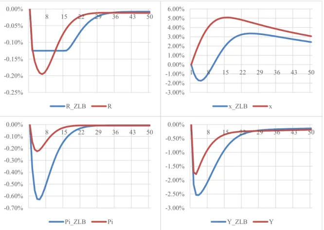
Figure 4. Impulse response functions of nominal interest rate (R), investment (x), inflation (Pie), and output (Y)

on a negative preference shock, under a ZLB-constrained (blue line) and an unconstrained Taylor rule (red line). Deviations are relative to the steady state levels.

5_{This “test-calibration” goes far beyond what has been dubbed the “new regime“ in preceding sections in order}

to construct an extreme scenario in which the ZLB becomes more relevant:Λ𝜇= Λ𝐴= 0.0001; Π =

1.001; 𝛽 = 0.9999. -0.25% -0.20% -0.15% -0.10% -0.05% 0.00% 1 8 15 22 29 36 43 50 R_ZLB R -3.00% -2.50% -2.00% -1.50% -1.00% -0.50% 0.00% 1 8 15 22 29 36 43 50 Y_ZLB Y -0.70% -0.60% -0.50% -0.40% -0.30% -0.20% -0.10% 0.00% 1 8 15 22 29 36 43 50 Pi_ZLB Pi -3.00% -2.00% -1.00% 0.00% 1.00% 2.00% 3.00% 4.00% 5.00% 6.00% 1 8 15 22 29 36 43 50 x_ZLB x

(14)

Assessing the situation with a binding ZLB, one can see in figure 4 that generally speaking the ZLB causes a higher drop in consumption, investment, and output. The policy rate cannot be as perfectly accommodative as it would be under an unconstrained Taylor rule. Hence, all of the aforementioned variables react more strongly than before. When closely examining the policy rate one can see that it first moves more quickly to the ZLB, stays there for a while, and then moves to positive territories slightly earlier than under the unconstrained Taylor rule. This can be ascribed to the fact that the system is fully deterministic and all agents have perfect foresight. Hence, the policy rate decreases more quickly in order to maximize the, now constrained, accommodative effect. In the long run all variables move back to their steady state in both cases.

5.1.2 Labor supply shock.

The labor supply shock enters the system in the household’s utility function as well. A negative labor supply shock causes households to supply more labor as the disutility of working is temporarily decreased. The shock is rather persistent due to a high persistence parameter of 0.93. As a consequence, the remaining macroeconomic variables move more slowly and persistently before returning to their steady state values in the long run. With higher labor input, output grows faster. Due to the characteristics of the intermediate goods sector’s production function, investment also increases. Labor becomes more affordable and thus, demand for capital increases to maintain efficient combinations of labor and capital upon producing intermediate goods. As output increases also consumption increases for a relatively long time as can be seen in figure 5. In the long run all variables return to their steady state levels. The increased supply of consumption goods and labor, puts pressure on wages and prices, causing inflation to decrease significantly. The policy rate decreases as a response to this effect, even though the increase in output prevents the Taylor rule to prescribe an even sharper decrease.

(15)

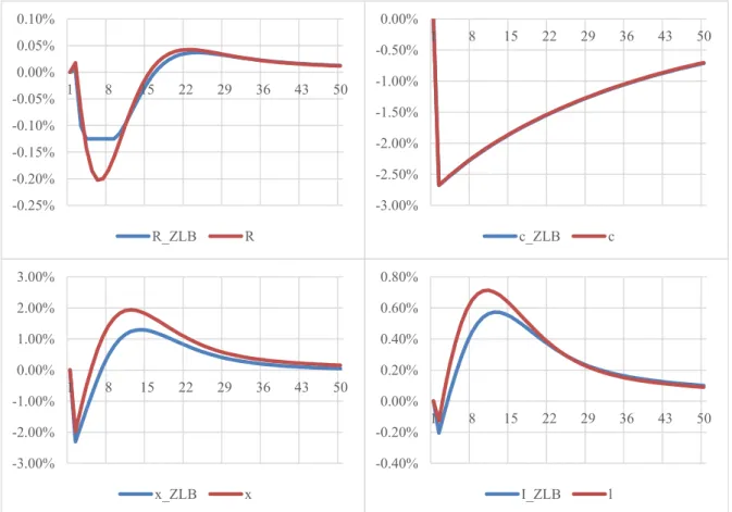
Figure 5. Impulse response functions of nominal interest rate (R), labor (l), inflation (Pie), and consumption (c)

on a negative labor supply shock, under a ZLB-constrained (blue line) and an unconstrained Taylor rule (red line). Deviations are relative to the steady state levels.

Comparing the two (ZLB-)constrained and the unconstrained scenarios, despite a possibly differing chain of causalities, the same signs of relative differences as under the intertemporal preference shock can be observed. For the constrained scenario, the policy rate moves more quickly to the ZLB, inflation falls more sharply, investment increases less strongly, hence output increases less significantly, than in the unconstrained scenario. The difference in consumption across these two scenarios is, just as before, very small.

5.1.3 Investment-specific technology shock.

The investment-specific technology shock, 𝜀𝜇,𝑡, enters the system directly in the equation

describing capital accumulation and indirectly in the intermediate goods sector’s production function. This shock is highly persistent. Applying a negative investment-specific technology shock increases the intermediary sector’s fixed production cost which, ceteris paribus, implies a reduction in intermediary goods output, and hence, final goods output. This has a direct, adverse impact on the households’ budget constraint implying a reduction in consumption and investment. Due to the decrease in utility, households prefer to decrease their labor supply as well, as the marginal utility of leisure has increased. Thus, all relevant endogenous variables -

0.00% 0.20% 0.40% 0.60% 0.80% 1.00% 1.20% 1.40% 1.60% 1 8 15 22 29 36 43 50 I_ZLB l -0.20% -0.15% -0.10% -0.05% 0.00% 0.05% 1 8 15 22 29 36 43 50 R_ZLB R 0.00% 0.02% 0.04% 0.06% 0.08% 0.10% 0.12% 0.14% 0.16% 0.18% 1 8 15 22 29 36 43 50 c_ZLB c -0.30% -0.25% -0.20% -0.15% -0.10% -0.05% 0.00% 0.05% 1 8 15 22 29 36 43 50 Pi_ZLB Pi

(16)

output, consumption, investment, and labor - fall at first upon a negative shock to investment-specific technology, as can be seen in figure 6.

Afterwards, a prolonged increase of investment follows, while the technology growth rate returned to its original level already. During this post-shock period investment increases above the steady state level as the productivity boost makes capital investments more profitable. Consequently, households use relatively more resources to invest and relatively less to consume as can be seen in figure 6. After reaching its tipping point on a level higher than under normal conditions, investment returns together with productivity to the steady state in the long run. Consumption continuously increases back to its steady state without

overshooting it. Due to the increase in capital, the demand for labor, and hence wages,

increases, which contributes to an increase in production and inflation. Output as well as labor reproduce the investment’s reaction of overshooting the steady state for several periods before slowly returning to it. Those developments are addressed by monetary policy in lowering the nominal rate of interest.

Figure 6.Impulse response functions of the nominal interest rate (R), consumption (c), investment (x), and labor (l) on a negative shock to investment specific technology, under a ZLB-constrained (blue line) and an

unconstrained Taylor rule (red line). Deviations are relative to the steady state levels. -0.40% -0.20% 0.00% 0.20% 0.40% 0.60% 0.80% 1 8 15 22 29 36 43 50 I_ZLB l -3.00% -2.00% -1.00% 0.00% 1.00% 2.00% 3.00% 1 8 15 22 29 36 43 50 x_ZLB x -3.00% -2.50% -2.00% -1.50% -1.00% -0.50% 0.00% 1 8 15 22 29 36 43 50 c_ZLB c -0.25% -0.20% -0.15% -0.10% -0.05% 0.00% 0.05% 0.10% 1 8 15 22 29 36 43 50 R_ZLB R

(17)

Comparing the (ZLB-)constrained and unconstrained scenarios, very similar relative

differences as with the preceding two shocks can be observed. Investment, output growth, and inflation are below their “non-ZLB levels”, whereas, naturally, the policy rate is mainly above this level, except that it moves to the ZLB earlier and stays there a bit longer than in the unconstrained scenario.

5.1.4 Shock to neutral technology.

The shock to neutral technology, 𝜀𝐴,𝑡, enters the system at the intermediary sector’s

production function in two ways. It directly impacts productivity as well as it enters the term determining fixed cost of production which ensures that economic profits remain close to zero in the steady state. This shock is also highly persistent. Upon a negative shock to neutral technology growth the system reacts in a uniformly, contractionary fashion, because neutral technology has a relatively higher weight in the cost part of the intermediary production function. Output, consumption, investment, and inflation initially decrease and revert slowly to their steady state levels, after neutral technology reverted to its steady state level of growth. Only investment shows some overshooting behavior when reverting to its steady state level, as can be seen in figure 7. One reason for this overshooting is that the capital stock requires some additional investment in order to reach its steady state level again in the long run. Nominal interest rates are set to accommodate a more stimulating environment when the system falls into recession.

(18)

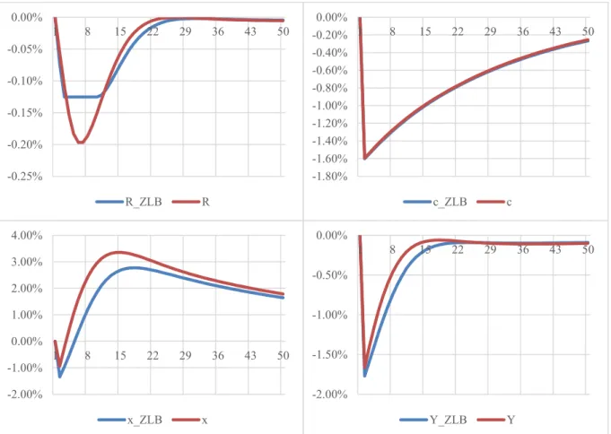
Figure 7. Impulse response functions of nominal interest rate (R), consumption (c), investment (x), and output

(Y) on a negative shock to neutral technology, under a ZLB-constrained (blue line) and an unconstrained Taylor rule (red line). Deviations are relative to the steady state levels.

Comparing the two scenarios with a binding and a non-binding ZLB, a similar behavior as with other shocks can be observed. In the constrained scenario investment, output, and inflation lie below their unconstrained levels. Also consumption is slightly below the level it would have in the unconstrained scenario. However, the relative difference is only marginal, whereas investment shows once again the highest relative deviation, as can be seen in figure 7. Nominal interest rates being constrained by the ZLB move there more quickly, remain above the level seen in the unconstrained scenario while reverting to the steady state for several periods.

5.2 Simulating a Set of Representative Shocks

After having understood the mechanics of this model in a deterministic setting and its interaction with the ZLB, this subsection’s goal is to define and to simulate a set of

representative shocks in order to assess the actual relevance of the ZLB. This assessment will be held first in the original “old regime” followed by simulations in the “new regime” which has been defined in section 4.

-2.00% -1.00% 0.00% 1.00% 2.00% 3.00% 4.00% 1 8 15 22 29 36 43 50 x_ZLB x -0.25% -0.20% -0.15% -0.10% -0.05% 0.00% 1 8 15 22 29 36 43 50 R_ZLB R -2.00% -1.50% -1.00% -0.50% 0.00% 1 8 15 22 29 36 43 50 Y_ZLB Y -1.80% -1.60% -1.40% -1.20% -1.00% -0.80% -0.60% -0.40% -0.20% 0.00% 1 8 15 22 29 36 43 50 c_ZLB c

(19)

5.2.1 Defining a set of shocks.

To assess whether a set of shocks can serve as a realistic representation of reality, historic data shall be the benchmark. More specifically, the goal is to find a combination of shocks which approximates an average recession observable during the last 40-50 years in the euro area respectively in the U.S.. The CEPR6_{Euro Area Business Cycle Dating Committee identifies}

five and the NBER7_{Business Cycle Dating Committee identifies seven recessions in the time}

period of 1970 to 2015.

By de-trending quarterly real GDP8_{using an HP (1600) filter these recessions can be}

measured. The size of a recession is calculated by taking the difference between a peak and a trough of the cyclical component of GDP. In order to estimate the size of a standard recession, the great recession during 2008 and 2009 is excluded from my calculations as it represents an extraordinary event.9_{Hence, there remain four recessions for the euro area of which the}

largest one had its trough in the first quarter of 1975 and a magnitude of 4.0%. The smallest one reached its trough in the first quarter of 2013 and amounted to 1.7% of real GDP. The average size of a recession for the euro area was 3.2%. For the U.S. there remain six

recessions of which the largest one, occurring in the first quarter of 1975 as well, was 6.6%, whereas the smallest one was 1.6%, reaching its trough in November 2001. The average size of a recession for the U.S. being 3.8%, was slightly larger than in the euro area.

Fernández-Villaverde (2010) provides a set of standard-sized shocks. These given magnitudes shall be the starting point to make an initial assessment whether they fit the above sketch of a representative recession in the euro area or the U.S.. Applying all of the four negative

standard shocks simultaneously, the maximum drawdown from steady state output trend is about 2.9% which is slightly below the range of 3.2% to 3.8%. Thus, this combination of shocks can be considered as an example for a small recession (scenario A). A combination of 1.5-fold standard shocks yields an output drop of 4.3% and will represent a large recession (scenario B). A combination of twofold standard shocks yields an output drop of 5.7% and represents a severe recession (scenario C), while a combination of 2.5-fold standard shocks yielding an output loss of 7.0% shall represent an extreme case scenario (scenario D) such as the Great Recession of 2008 and 2009 for instance. Besides combinations of several shocks,

6_{Centre for Economic Policy Research} 7_{National Bureau of Economic Research}

8_{Euro area data is taken from the Area Wide Model (AWM) dataset by Gabriel Fagan, Jérôme Henry and}

Ricardo Mestre. U.S. data is taken from the Federal Reserve Economic Data (FRED) database.

9_{According to the applied calculations methods the Great Recession came along with an output loss of 5.2% in}

(20)

also multiples of individual shocks will be simulated and analyzed separately in order to evaluate the differing relevance of the ZLB.

5.2.2 Simulating shocks under pre-crisis conditions.

Once the set of shocks has been defined, the model reactions towards them shall be analyzed more thoroughly. The first set of simulations is run under the “old regime” which is

representative to the economic reality before the Great Recession of 2008-2009. The drops in output growth have already been mentioned in the preceding paragraph. Even though the simple standard shocks simulated do not even cause large recessions, it typically takes a high number of periods – one period equals one quarter – until output returns to its steady state. Under the set of simple standard shocks causing a small recession of 2.9% of steady state output (scenario A), it takes around 44 periods for output to go back to steady state (deviation <0.10%). Even upon applying shocks individually the time for output to revert to the steady state is about 44 periods for a standard shock to neutral technology, 52 periods for a standard labor supply shock or 22 periods for a standard intertemporal preference shock.

Even though the various impulse response functions on individual shocks have already been described and analyzed in the preceding sections, they have not been discussed upon

combinations of several shocks nor have the individual shocks been compared with respect to their different sizes of impact. First of all, comparing the individual standard shocks, yields that the shock to neutral technology has the biggest, while the shock to investment specific technology, as well as the shock to labor supply have hardly any negative effect on output.10

The same observation holds when comparing the individual standard shocks with respect to their “ZLB relevance”: The shock to investment specific technology and the shock to labor supply have the least impact, while the shock to neutral technology has the largest negative impact on nominal interest rates. Once the shocks’ standard magnitudes are multiplied, further observations can be made. As can be seen in figure 8, the labor supply shock has hardly any effect on output and is more effective in driving the system closer to the ZLB, whilst the shocks to neutral technology and intertemporal preferences have a relatively higher effect on output, compared to nominal interest rates.

Even though some of the individual standard shocks trigger considerable decreases in nominal interest rates, the ZLB has no significant relevance for them in the “old regime”. Only an 11-fold standard shock to labor supply manages to push the policy rate to the ZLB. However, the

(21)

ZLB constraint has hardly any effect on the maximum output loss under this type of shock. Hence, this scenario can easily be neglected for any purposes. Furthermore, under a

combination of all four standard shocks, the policy rate does not go below 4.97%,

representing a drop of only 190 basis points from the steady state (which is 6.78% in this regime). Upon simulating a 2.5-fold combination of standard shocks, which represents the

extreme case scenario, there still remains a buffer of 235 basis points towards the ZLB. Only

upon applying a 3.5-fold combination of standard shocks – which implies an unrealistically high output drop of 9.4% – the system moves relatively close to the ZLB.11_{Hence, the ZLB is}

basically non-binding under the “old regime” which is confirmed by actual data of the past 40-50 years. Usually, the buffer towards the ZLB is sufficiently large.

Figure 8. Overview of maximum output losses and minimum nominal interest rates under different shock

scenarios in the “old regime”. Only representative scenarios of combinations of shocks are displayed: A = 1-fold, B = 1.5-fold, C = 2-fold, and D = 2.5-fold combination of standard shocks. Further scenario details as well as other scenarios can be looked up in table E1 of Annex E.

5.2.3 Simulating shocks under post-crisis conditions.

Considering the “new regime”, yields different conclusions. The ZLB becomes naturally a more relevant constraint as the new steady state is characterized by a lower nominal interest rate. The distance to the ZLB is 366 basis points in this calibration while it was 678 basis points before, as displayed in figure 9. Furthermore, due to the characteristic set-up of the monetary policy rule, which remains unchanged upon the “regime” change, the same shock scenarios trigger larger drops in nominal interest rates than under the “old regime”. This

11_{Further details on this and other type of shocks can be looked up in table E1 of Annex E.}

D C B A 0 100 200 300 400 500 600 0% 1% 2% 3% 4% 5% 6% 7% 8% m in . R (in b ps )

(22)

difference is, for most scenarios, roughly 10% to 20% of the “old regime’s” interest rate decrease12_.

Figure 9. Impulse response functions of the nominal interest rate (R) during shock scenario A in the “old” (blue

line) and “new regime” (red line). Rates are p.a..

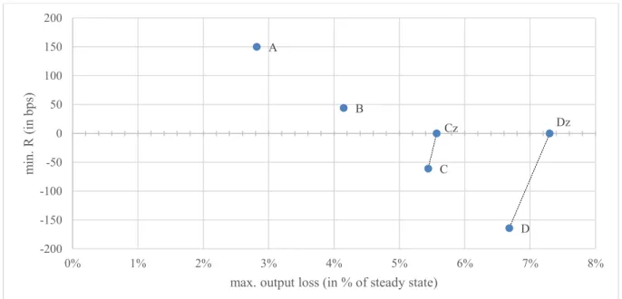
Hence, driving the system close to the ZLB (or below) does not require as large shocks as before anymore. A large recession (scenario B) yields a nominal interest rate of 44 basis points above zero. The scenarios C, D, E, and F, representing combinations of twofold

standard shocks and higher orders, cause the system to hit the ZLB. Another effect observable in the “new regime” calibration is the fact that all shocks, except the shock to labor supply, trigger slightly smaller output deviation from the steady state compared to simulations in the “old regime”. For example, a combination of simple standard shocks (scenario A) induces a fall in output of only 2.82%, whereas it fell by 2.94% in the “old regime” calibration for the same scenario of shocks. This can be explained by the specific construction of the monetary policy rule in this model which induces interest rate reactions as a function of relative (and not absolute) deviations from steady state output and steady state inflation. Hence, as the same type of shock induces a relatively larger deviation from steady state in the new regime, monetary policy replies more strongly as can be seen in figure 9. Nominal interest rates are decreased more strongly in the “new regime” (216 bps instead of 181 bps). Consequently, absolute output loss is kept slightly smaller.

Looking at the actual ZLB relevance, it can be concluded that hitting the ZLB would require at least a combination of shocks consistent with a severe recession and is thus still a relatively

12_{This is mostly true for scenarios with significant interest rate drops (>100 bps).}

-181 bps from steady state -216 bps from steady state 0% 1% 2% 3% 4% 5% 6% 7% 8% 1 3 5 7 9 11 13 15 17 19 21 23 25 27 29 31 33 35 37 39 41 43 45 47 49

(23)

unlikely event. Similar sized recessions13_{have occurred three times in the U.S. and zero times}

in the euro area economy during the last 45 years.

Figure 10. Overview of maximum output losses and minimum nominal interest rates under different shock

scenarios in the “new regime”. Only representative scenarios of combinations of shocks are displayed: A = 1-fold, B = 1.5-1-fold, C = 2-1-fold, and D = 2.5-fold combination of standard shocks. Further scenario details as well as other scenarios can be looked up in table E1 of Annex E.

In order to gain a better understanding of the effects of the ZLB in this “new regime”

environment, scenarios D and C are examined more carefully. As mentioned before, enforcing the ZLB constraint causes a higher output loss and hence, a higher loss in consumption. Losses in consumption are, however, relatively small compared to differences in output. Another significant difference is the lower inflation rate. If the policy rate cannot be lowered below the ZLB, inflation rates decrease relatively stronger as can be seen in figure 11. Since the constrained policy rate causes a less accommodative environment, the temporary counter reaction of output growth above the steady state is not as strong as in the unconstrained case.

13_{Maximum output loss of at least 5% of GDP.}

D Dz C Cz B A -200 -150 -100 -50 0 50 100 150 200 0% 1% 2% 3% 4% 5% 6% 7% 8% m in . R (in b ps )

(24)

Figure 11. Impulse response functions of nominal interest rates (R), consumption (c), inflation (Pi), and output

(Y) in shock scenario D in the “new” (red lines) and the “old regime” (blue lines). Dashed lines represent scenarios with an unconstrained monetary policy rule. Inflation and interest rates are p.a., output and consumption are relative to their steady state.

Comparing the “new” and the “old regime” impulse response functions under a constrained monetary policy is also an interesting analysis. To this end, shock scenario D which

represents an extreme case recession, depicted in figure 11, is analyzed further. The first and most obvious observation is that the nominal interest rate is decreasing significantly less in the “new regime”. Secondly, because monetary policy is not as accommodative as it should be, the inflation rate decreases much stronger. While it decreased by about 5.7 percentage points in the “old regime”, it dropped by more than 10 percentage points in the “new regime”. When looking at output and consumption, the differences are comparatively smaller. Output decreases at its lowest point 34 basis points more, and consumption only 6 basis points more in the “new regime” with a constrained monetary policy rule.

This allows two conclusions. First, the ZLB is more likely to become a binding constraint in the “new regime” calibration representing the current economic regime. It required a

combination of shocks sized at least twice the size of standard shocks which includes a severe

recession and an extreme case scenario such as the Great Recession. Hence, hitting the ZLB

can still be considered an unlikely event. -4% -2% 0% 2% 4% 6% 8% 1 9 17 25 33 41 49 R_D_old R_Dz_new R_D_new -8% -6% -4% -2% 0% 2% 4% 6% 1 9 17 25 33 41 49 Y_D_old Y_Dz_new Y_D_new -8% -7% -6% -5% -4% -3% -2% -1% 0% 1 9 17 25 33 41 49

c_D_old c_Dz_new c_D_new

-10% -8% -6% -4% -2% 0% 2% 4% 6% 1 9 17 25 33 41 49 Pi_D_old Pi_Dz_new Pi_D_new

(25)

Secondly, in this model, hitting the ZLB, yields under this specific calibration, relatively small losses in consumption and output. Hence, the harm in terms of GDP caused by the ZLB constraint is almost negligible under combinations of shocks up to a certain size. It is fair to say that the potential output and consumption losses caused by the ZLB constraint increase exponentially with the size of the shock.

6 Sensitivity Analysis

A sensitivity analysis is performed in order to test the robustness of the above results. The robustness of results is tested under monetary policy rules calibrated in different ways than the original model calibration by Fernández-Villaverde (2010) suggests. The base assumption is that the key results remain conceptually the same for most calibrations of the Taylor rule. The Taylor rule is specified by three parameters (𝛾𝑅, 𝛾𝑦, 𝛾𝜋) in this model, which are modified

in order to construct different reaction functions. I re-ran my simulations with two alternative monetary policy rule specifications, by Christiano, Eichenbaum and Trabandt (2015) and by Bokan, Gerali, Gomes, Jacquinot and Pisani (2016), and with the original standard

specification proposed by Taylor (1993) which inhibits no smoothing of interest rates. Table 2 summarizes the tested calibration alternatives.

Coefficient on lagged interest rates (𝜸𝑹) Coefficient on inflation (𝜸𝝅) Coefficient on the output gap (𝜸𝒚) Bokan et al. (2016) 0.870 1.700 0.100 Christiano et al. (2015) 0.751 1.666 0.247 Fernández-Villaverde (2010) 0.770 1.290 0.190 Taylor (1993) 0.000 1.500 0.500

Table 2. Overview of different monetary policy rule specifications applied in the sensitivity analysis. The results of the different sensitivity simulations strongly depend on the monetary policy rule specification. Generally, the original Taylor rule prescribes the strongest drop in interest rates. Hence, the ZLB becomes binding more easily. Bokan et al.’s (2016) resp. Christiano et al.’s (2015) calibration trigger monetary policy reactions slightly weaker resp. stronger than Fernández-Villaverde’s (2010) original calibration as can be seen in figure 12.

(26)

Figure 12. Overview of maximum output losses and minimum nominal interest rates under different shock scenarios and monetary policy rules, in the “old regime”. Only representative scenarios of combinations of shocks are displayed: A = 1-fold, B = 1.5-fold, C = 2-fold, and D = 2.5-fold combination of standard shocks. Further scenario details as well as other scenarios can be looked up in table F1-3 of Annex F.

Starting with observations made on simulations in the “old regime” environment, it can be concluded that, except for the original Taylor rule (1993), results are broadly the same. The ZLB is no constraint under the representative shocks, which is due to the fact that the two alternative specifications do not significantly deviate from the model’s originally calibrated monetary policy rule. The original Taylor rule prescribes interest rates close to zero already upon a 1.5-fold shock. Twofold shocks and beyond cause the ZLB to become a binding constraint associated with output losses of up to 0.12% (scenario C) resp. 0.50% (scenario D) of steady state GDP.

In the “new regime” environment the ZLB moves closer to the steady state. Hence, the interest rate reactions prescribed by the original Taylor rule are now theoretically all below zero as can be seen in figure 13. While monetary policy would be effectively constrained by the ZLB in scenario C and D under the calibration proposed by Bokan et al. (2016), the ZLB would represent no effective constraint in all scenarios under the specification proposed by Christiano et al. (2015). D C B A C D B A -600 -400 -200 0 200 400 600 800 0% 1% 2% 3% 4% 5% 6% 7% 8% m in . R (in b ps )

max. output loss (in % of steady state)

(27)

Figure 13. Overview of maximum output losses and minimum nominal interest rates under different shock scenarios and monetary policy rules in the “old regime”. Only representative scenarios of combinations of shocks are displayed: A = 1-fold, B = 1.5-fold, C = 2-fold, and D = 2.5-fold combination of standard shocks. Further scenario details as well as other scenarios can be looked up in table F4-6 of Annex F.

Thus, considering that the original Taylor rule with no persistence in interest rates is not a good benchmark of monetary policy today, it can be concluded that the results in the previous sections are qualitatively robust. Nevertheless, the choice of monetary policy rule has some impact on how early the ZLB becomes a binding constraint. There are specifications under which the ZLB has no binding effect, even though the buffer towards it becomes almost zero under an extreme recession. Considering that the ZLB has become a binding constraint during the Great Recession in most advanced economies, these policy rules may not be a good benchmark to analyze monetary policy as currently conducted by central banks.

7 Mitigating the Zero Lower Bound Risk

With respect to the preceding sections discussing how the ZLB becomes a more binding constraint under low inflation regimes, increasing the inflation target has obviously the advantage of increasing the potential buffer towards the ZLB. The steady state policy rate would move up alongside an inflation target increase. Hence, the buffer between the steady state nominal interest rate and the ZLB would increase by the same amount. This measure would mechanically mitigate the effect of lower steady state growth with respect to the buffer to the ZLB.

Not only would this increase the scope for monetary policy to provide stimulus during shocks, but also would it provide additional flexibility for the adjustment of real prices and wages. Downward nominal wage rigidities would be better mitigated under a higher steady state

D C B A D C B A -1000 -800 -600 -400 -200 0 200 400 0% 1% 2% 3% 4% 5% 6% 7% 8% m in . R (in b ps )

max. output loss (in % of steady state)

(28)

inflation (Daly & Hobijn, 2014). This is beneficial as it allowed the labor market to adjust under a negative shock more quickly by lowered wages and less by increased unemployment. Nevertheless, no major central bank has increased or even openly discussed increasing the inflation target. That is in part related to political resistance, which is particularly high in countries like Germany, for instance, which has a history of costly hyperinflation.

Furthermore, increasing the inflation target has substantial economic disadvantages. A higher steady state inflation is typically associated with distortions in cash holdings, overinvestment in the financial sector, greater uncertainty about relative prices and the aggregate price level, distortions in the tax system, and redistribution of wealth (Mishkin, 2011). Another

significant impediment is related to credibility. Not only is it questionable if central banks could fully convince market participants of a higher inflation target but also is there the threat of un-anchoring inflation expectations. Bernanke (2010) argues that increasing the inflation target once, would significantly increase uncertainty about inflation expectations and would have negative effects on the overall credibility of a central bank. One common criticism is the potentially increased overall volatility. However, Justiniano, Primiceri and Tambalotti (2013) come to the conclusion that, at least in a DSGE environment, there is no trade-off between inflation and output stabilization.

Still, increasing the inflation target appears not to be necessary at this point, as central banks apply a set of unconventional monetary policy tools allowing them to decrease interest rates beyond levels possible with conventional measures. Most prominently, all major central banks performed large-scale asset purchases as well as reinforced their forward guidance. Both measures have proven to be successful at reducing the harm caused by the ZLB constraint (Chung et al., 2012; Coenen & Warne, 2013). Chung et al. (2012) estimate, for instance, the U.S. quantitative easing programs to having had a stimulating effect to the job market from 2009 to 2012, equivalent to a counterfactual policy rate decrease of about 300 basis points, which would have not been possible due to the ZLB constraint.

Another unconventional measure which gained some more attention recently is the so-called “helicopter money” which refers to a way of directly financing the economy through the central bank circumventing the banking system as an intermediary. Buiter (2014), among others, argues that, given a set of conditions, the threats of deflation or low inflation can effectively be avoided by this way of direct private sector financing. “Helicopter money” has its strong opponents as well, for legitimate reasons. The most obvious reason is that central banks would risk their independence by such powerful interventions which usually fall into

(29)

the domain of fiscal policy. Issing (2015) claims that once a central bank breaks this taboo of directly financing the private sector, it is likely to experience strong political pressure to provide this measure more regularly or permanently. It remains questionable if the central bank would be able to withstand this kind of political pressure. Hence, existing

unconventional measures are likely to remain the tool of choice to complement conventional monetary policy and to mitigate the ZLB.

8 Conclusion

To conclude, it has been shown that the new economic environment of lower real interest rates, lower steady state inflation, and lower potential growth causes the ZLB constraint to become a more likely event which does affect the dynamics of an economy following a set of shocks. Nevertheless, it has been illustrated that it still remains unlikely and that the

associated costs seem to be comparatively small in my simplified setting. This second finding does to some extent qualify recent results of economic literature, such as for instance by Dordal-i-Carreras et al. (2016) who concluded that once the ZLB becomes binding it is typically very costly due to the long duration. It may be the case however, that the simplified model that has been used for my simulations systematically underestimates the duration of ZLB periods. Thus, it may not be suitable to make qualified statements about the welfare costs associated with the ZLB constraint.

Furthermore, it has been concluded that increasing the buffer to the ZLB during steady state – for example by increasing the inflation target – should be no urgent goal of policy makers. This conclusion is reinforced if it is being taken into account that there are various ways of mitigating the ZLB effects or of increasing this buffer, including large-scale asset purchase programs and forward guidance.

Looking at current states of the economies in the euro area and the U.S., it remains

questionable though, if the new steady state has adjusted already. With nominal interest rates close to the ZLB, the above simulations and illustrations have little relevance, as any kind of shock makes the ZLB, with almost certainty, a binding constraint. Thus, the longer the economies are in this state, the more relevant becomes the question on how to effectively address the ZLB constraint. The simulations performed assume a new steady state with nominal interest rates at about 370 basis points above zero. If it turns out that the current environment of 2016 is much closer to the new steady state than previously anticipated the above findings lose much of their validity. The revised conclusion would be that the ZLB is a highly immediate and certain constraint during most of the time. Additional measures such as

(30)

increasing the inflation target or more unconventional measures including asset purchases and possibly “helicopter money” would need to be on the agenda of central banks in the near future.

Hence, one subject which obviously needs to be researched more thoroughly is the investigation of the “new normal” i.e. the new steady state of the euro area and the U.S. economies. Only if this question has been clarified, a more pragmatic discussion on the necessary policy tools can be held. The transmission of monetary policy under very low interest rates, in particular with regards to the interaction with the financial sector, also calls for further research.

(31)

References

Andrés, J., López-Salido, J. D., & Nelson, E. (2009). Money and the natural rate of interest: Structural estimates for the United States and the euro area. Journal of Economic

Dynamics and Control, 33(3), 758-776.

Ball, L. M. (2014). The case for a long-run inflation target of four percent. IMF Working

Paper, 92(14).

Barsky, R., Justiniano, A., & Melosi, L. (2014). The natural rate of interest and its usefulness for monetary policy. The American Economic Review, 104(5), 37-43.

Bernanke, B. S. (2010, August). The economic outlook and monetary policy. In Speech at the Federal Reserve Bank of Kansas City Economic Symposium, Jackson Hole, Wyoming (Vol. 27).

Bernanke, B. S. (2016, August 8). The Fed’s shifting perspective on the economy and its implications for monetary policy. Retrieved August 9, 2016, from

https://www.brookings.edu/2016/08/08/the-feds-shifting-perspective-on-the-economy-and-its-implications-for-monetary-policy/.

Blanchard, O., Dell’Ariccia, G., & Mauro, P. (2010). Rethinking macroeconomic policy.

Journal of Money, Credit and Banking, 42(s1), 199-215.

Bokan, N., Gerali, A., Gomes, S., Jacquinot, P., & Pisani, M. (2016). A macroeconomic model of banking and financial interdependence in the euro area. ECB Working

Papers Series, 1923.

Buiter, W. H. (2014). The Simple Analytics of Helicopter Money: Why It Works – Always.

Economics: The Open-Access, Open-Assessment E-Journal, Vol. 8, 2014-28.

Christiano, L. J., Eichenbaum, M. S., & Trabandt, M. (2015). Understanding the great recession. American Economic Journal: Macroeconomics, 7(1), 110-167. Chung, H., Laforte, J. P., Reifschneider, D., & Williams, J. C. (2012). Have we

underestimated the likelihood and severity of zero lower bound events?. Journal of

Money, Credit and Banking, 44(s1), 47-82.

Coenen, G., & Warne, A. (2013). Risks to price stability, the zero lower bound and forward guidance: a real-time assessment. International Journal of Central Banking, 2014(2).

(32)

Coenen, G., Orphanides, A., & Wieland, V. (2003). Price stability and monetary policy effectiveness when nominal interest rates are bounded at zero. CFS Working Paper,

2003(13).

Coibion, O., Gorodnichenko, Y., & Wieland, J. (2012). The optimal inflation rate in New Keynesian models: should central banks raise their inflation targets in light of the zero lower bound?. The Review of Economic Studies, 79(4), 1371-1406.

Cúrdia, V., Ferrero, A., Ng, G. C., & Tambalotti, A. (2015). Has US monetary policy tracked the efficient interest rate?. Journal of Monetary Economics, 70, 72-83.

Daly, M. C., & Hobijn, B. (2014). Downward nominal wage rigidities bend the Phillips curve.

Journal of Money, Credit and Banking, 46(S2), 51-93.

Dordal-i-Carreras, M., Coibion, O., Gorodnichenko, Y., & Wieland, J. (2016). Infrequent but Long-Lived Zero-Bound Episodes and the Optimal Rate of Inflation. NBER Working

Paper Series, 22510.

Eggertsson, G. B., & Woodford, M. (2003). The Zero Bound on Interest Rates and Optimal Monetary Policy. Brookings Papers on Economic Activity (2003).

European Central Bank (ECB). Inflation and the euro. (2016). Retrieved August 25, 2016, from https://www.ecb.europa.eu/stats/prices/hicp/html/inflation.en.html.

Fagan, G., Henry, J., & Mestre, R. (2005). An area-wide model for the euro area. Economic

Modelling, 22(1), 39-59.

Federal Reserve Bank of St. Louis (FRED). Inflation. (2016). Retrieved August 25, 2016, from https://fred.stlouisfed.org/tags/series?t=inflation.

Federal Reserve Bank of St. Louis (FRED) (2016). Real gross domestic product per capita. Retrieved November 11, 2016, from

https://fred.stlouisfed.org/series/A939RX0Q048SBEA.

Fernald, John G. (2016). Reassessing Longer-Run U.S. Growth: How Low?. Federal Reserve

Bank of San Francisco Working Paper, 2016-18.

(33)

Fernández-Villaverde, J., Gordon, G., Guerrón-Quintana, P., & Rubio-Ramirez, J. F. (2015). Nonlinear adventures at the zero lower bound. Journal of Economic Dynamics and

Control, 57, 182-204.

Fernández-Villaverde, J., & Rubio-Ramírez, J. F. (2006). A baseline DSGE model. University

of Pennsylvania.

Goldby, Mike, Lien Laureys and Kate Reinold. 2015. “An estimate of the UK’s natural rate of interest,” Bank Underground (Bank of England blog), August 11, 2015.

http://bankunderground.co.uk/2015/08/11/an-estimate-of-the-uks-natural-rate-of-interest/.

Gordon, R. J. (2014). The turtle’s progress: Secular stagnation meets the headwinds. In

Secular stagnation: Facts, causes and cures (pp. 47-59). Centre for Economic Policy

Research.

Griffoli, T. M. (2013). Dynare User Guide: An introduction to the solution & estimation of DSGE models. Retrieved July 1, 2016, from http://www.dynare.org/documentation-and-support/user-guide/Dynare-UserGuide-WebBeta.pdf.

Hamilton, J. D., Harris, E. S., Hatzius, J., & West, K. D. (2015). The equilibrium real funds rate: Past, present and future. NBER Working Paper Series, 21476.

Holston, K., Laubach, T., & Williams, J. (2016, July). Measuring the natural rate of interest: International trends and determinants. In NBER International Seminar on

Macroeconomics 2016. Journal of International Economics (Elsevier).

Justiniano, A., Primiceri, G. E., & Tambalotti, A. (2013). Is there a trade-off between inflation and output stabilization?. American Economic Journal: Macroeconomics, 5(2), 1-31. Kiley, M. T. (2015). What can the data tell us about the equilibrium real interest rate?.

Finance and Economics Discussion Series, 2015(077). Washington: Board of

Governors of the Federal Reserve System, http://dx.doi.org/10.17016/FEDS.2015.077. Laubach, T., & Williams, J. C. (2016). Measuring the natural rate of interest redux. Finance

and Economics Discussion Series, 2016(011). Washington: Board of Governors of the

(34)

Lubik, T. A., & Matthes, C. (2015). Calculating the natural rate of interest: A comparison of two alternative approaches. Richmond Fed Economic Brief, 2015(Oct), 1-6.

Mishkin, F. S. (2011). Monetary policy strategy: lessons from the crisis. NBER Working

Paper Series, 16755.

Neiss, K. S., & Nelson, E. (2003). The real-interest-rate gap as an inflation indicator.

Macroeconomic Dynamics, 7(02), 239-262.

Reifschneider, D., & Williams, J. C. (2000). Three lessons for monetary policy in a low-inflation era. Journal of Money, Credit and Banking, 32(4), 936-966.

Schmitt-Grohé, S., & Uribe, M. (2010). The optimal rate of inflation. NBER Working Paper

Series, 16054.

Summers, L. H. (2014a). Reflections on the ‘New Secular Stagnation Hypothesis’. In Secular

stagnation: Facts, causes and cures (pp. 27-40). Centre for Economic Policy

Research.

Summers, L. H. (2014b). US economic prospects: Secular stagnation, hysteresis, and the zero lower bound. Business Economics, 49(2), 65-73.

Taylor, J. B. (1993). Discretion versus policy rules in practice. Carnegie-Rochester

conference series on public policy, 39(1993), 195-214.

Teulings, C., & Baldwin, R. (2014). Secular stagnation: Facts, causes, and cures. Retrieved August 01, 2016, from http://www.tau.ac.il/~yashiv/Vox_secular_stagnation.pdf. Wicksell, K. (1936). Interest and Prices, 1898. Translated by RF Kahn.

Williams, J. C. (2003). The natural rate of interest. FRBSF Economic letter, 2003(32). Williams, J. C. (2009). Heeding Daedalus: Optimal inflation and the zero lower

bound. Brookings Papers on Economic Activity, 2009(2), 1-37.

Williams, J. C. (2014). Monetary policy at the zero lower bound: Putting theory into practice.

Hutchins Center Working Papers, 2014(January 16).

Williams, J. C. (2015). The decline in the natural rate of interest. Business Economics, 50(2), 57-60.

(35)

Williams, J. C. (2016). Monetary policy in a low R-star world. FRBSF Economic Letter,