Development of a medical app for clinical use

Faculdade de Engenharia da Universidade do Porto

Development of a clinical app to predict the

biomechanical behaviour of femur bones

Guilherme Faria Henriques

F

V

Dissertation performed in the scope of the

Integrated Masters in Bioengineering

Major in Biomedical Engineering

Supervisor: Jorge Américo Oliveira Pinto Belinha

Co-supervisor: Renato Manuel Natal Jorge

i

Abstract

Hip surgeries affect a large number of people with reports showing up to 7 million Americans being submitted to hip replacement surgery by 2015 and that number is expected to rise continuously. Despite this fact, in the present, there is no tool in a clinical environment which can provide relevant mechanical information to the physician in order to reduce the need for a revision surgery. Some relevant work has been done academically, regarding image segmentation, however those methods generally apply to secondary image modalities, such as MRI and CT scans. As defined by the AAOS, the clinical guidelines point towards using radiographs as the first imaging tool in hip injuries making this image modality of greater use in the clinical field.

In this dissertation, a background of information is given regarding the femoral bone and its anatomical, biological, pathological and mechanical perspectives. Following that, medical image modalities are explored and the theoretical principles behind them are explained. This is followed by a survey on the state of the art of image segmentation methods related to the topic of the present project. Moreover, a finite element method overview is given not only regarding its formulation but also its history with a heavier focus on the field of orthopaedics. Lastly, the proposed clinical application is presented which, using femur x-ray radiographs, can process the femur computational model automatically and performs finite element analysis to assess the stress distribution in the bone. To perform this, the algorithm resorts to the radiograph’s gradient to attain the computational model and with the evenly spread out mesh, executes a finite element analysis on the stress distribution calculating effective stress and its ratio to ultimate stress.

The obtained results allow the physician to assess the overall stress and damage level distribution if some considerations are taken when analysing the radiographs, such as the presence of artefacts and the presence of a meaningful contrast between trabecular and cortical bone.

iii

Resumo

Cirurgias de anca afetam milhões de pessoas em todo o mundo, com estudos a demonstrarem que até 2015, cerca de 7 milhões de Americanos já sofreram uma artroplastia de anca ou de joelho. Este número é ainda espectável que continue a subir. Apesar disto, não existe atualmente uma ferramenta usada em ambiente clínico que providencie informação mecânica relevante para que uma cirurgia de revisão não seja necessária. Apesar de algum trabalho ter sido desenvolvido em âmbito académico em relação a segmentação de imagem, os métodos desenvolvidos geralmente aplicam-se à modalidade de imagens como ressonâncias magnéticas, ou TC’s. A AAOS define, nas suas guidelines clínicas, que num paciente ortopédico a modalidade de imagem a ser usada deverá ser a radiografia e apenas em caso de dúvida se deve recorrer a outras modalidades. Este facto reitera a necessidade de existir mais tecnologia desenvolvida para a modalidade mencionada.

Nesta dissertação, é fornecida informação de contextualização em relação ao fémur e às suas perspetivas anatómica, biológica, patológica e mecânica. De seguida é explorado o tema de modalidade de imagens médicas, em que os princípios teóricos que as regem serão apresentados. Posteriormente, é apresentada uma pesquisa sobre o estado de arte de métodos de segmentação de imagem aplicados ao projeto em questão, procurando focar em radiografias. Após esta apresentação, é dada uma perspetiva global sobre o Método de Elementos Finitos não só sobre a sua formulação, mas também abordando a sua história com um foco especial na área da ortopedia.

Por último, é apresentada a aplicação clínica proposta na qual, usando radiografias de fémur, é possível realizar um processamento automático do modelo computacional e realizar análise de elementos finitos para avaliar a distribuição de tensões no osso. Para obter estes resultados o algoritmo recorre ao gradiente da radiografia para chegar ao modelo computacional, sendo capaz de gerar automaticamente uma malha uniforme e efetuar a análise de tensões, calculando a tensão efetiva e o seu rácio com a tensão máxima de compressão.

Os resultados obtidos permitem ao clínico avaliar a distribuição de tensões, tendo em conta algumas considerações com as radiografias, como a presença de artefactos e a presença de um contraste significativo entre osso trabecular e osso cortical.

v

Institutional Acknowledgements

The author truly acknowledges the work conditions provided by the Applied Mechanics Division (SMAp) of the Department of Mechanical Engineering (DEMec) of Faculty of Engineering of the University of Porto (FEUP), and by the MIT-Portugal project “MIT-EXPL/ISF/0084/2017”, funded by Massachusetts Institute of Technology (USA) and “Ministério da Ciência, Tecnologia e Ensino Superior - Fundação para a Ciência e a Tecnologia” (Portugal).

Additionally, the authors gratefully acknowledge the funding of Project NORTE-01-0145-FEDER-000022 - SciTech - Science and Technology for Competitive and Sustainable Industries, cofinanced by Programa Operacional Regional do Norte (NORTE2020), through Fundo Europeu de Desenvolvimento Regional (FEDER).

Furthermore, the author acknowledges the inter-institutional collaboration with the orthopaedics service of Central Hospital of Porto – Hospital de Santo António – and its director, Prof.Dr. António Fonseca Oliveira.

Finally, the author acknowledges the synergetic collaboration with the collaborators of “Computational Mechanics Research Laboratory CMech-Lab” (ISEP/FEUP/INEGI), and its director, Prof.Dr. Jorge Belinha, and its senior advisors, Prof.Dr. Renato Natal Jorge and Prof.Dr. Lúcia Dinis.

vii

Personal Acknowledgements

Ao longo do processo da dissertação e todo o caminho para aqui chegar, não caminhei sozinho. Felizmente, pude contar com amigos e família que me ajudaram nos tempos mais difíceis e com quem partilhei os momentos mais felizes.

À minha família, ao meu pai, minha mãe e minha irmã, quero agradecer a força e confiança que me deram sem me deixarem ir abaixo. Obrigado também pela ajuda, desde os aspetos técnicos até às situações mais casuais que me permitiram chegar onde cheguei.

Obrigado Isabel pelo teu amor, por acreditares em mim mesmo se eu não o fazia e por me ajudares a ultrapassar os meus objetivos, mesmo que nada tenham a ver com o curso. Também por ti sou a pessoa que sou hoje e a ti te devo isso.

Obrigado aos meus avós por sempre se preocuparem comigo e verem em mim uma pessoa em quem podem contar e orgulhar-se.

Obrigado às Alheiras pelos momentos de alegria, pelos jantares e pelos passeios. Espero que continuemos a reunirmo-nos para que esta tradição não se perca.

Obrigado aos meus amigos, pelo companheirismo seja nos momentos de encontro seja pela partilha de vídeos de Gato Fedorento.

Por último, gostaria de dedicar todo este meu percurso académico à minha avó que não estando presente para me ver terminar, tenho a certeza que ficaria cheia de orgulho por este momento.

A todos os mencionados e aos que, por lapso meu, não foram mencionados o meu muito obrigado.

ix

Table of contents

Abstract ... i

Resumo ... iii

Institutional Acknowledgements ... v

Personal Acknowledgements ... vii

Table of contents ... ix

List of figures ... xi

List of tables ... xv

Abbreviations ... xvii

Chapter 1 - Introduction ... 1

1.2 - Goal of the project ... 1

1.3 - Document's structure... 2

Chapter 2 - Femoral Bone ... 3

2.1 - Introduction ... 3

2.2 - Anatomy ... 3

2.3 -Biology ... 5

2.4 -Pathologies ... 7

2.5 -Mechanical properties ... 8

Chapter 3 - Medical Imaging ... 13

3.1 - Introduction and history ... 13

3.2 - Magnetic Resonance Imaging – MRI ... 14

3.3 - Computed Tomography – CT ... 15

3.4 - X-ray Radiographs... 16

Chapter 4 - Image Segmentation ... 17

4.1 - Introduction ... 17

4.2 - General overview ... 17

4.3 - 2D x-ray segmentation techniques... 18

Chapter 5 - Finite Element Method ... 25

5.1 - Origins ... 25

5.2 - Formulation ... 25

Chapter 6 - Finite Element Method in Orthopaedics ... 35

6.1 - The start... 35

6.2 - The first decade ... 35

6.3 - Problem-oriented development ... 36

6.4 - Recent developments ... 37

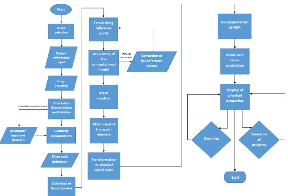
Chapter 7 - Femur Analysis Tool ... 39

7.1 - Introduction ... 39

x

7.3 - Software Algorithm ... 41

7.3.1 - Determining the image orientation ... 41

7.3.2 - Gradient computation and thresholding ... 42

7.3.3 - Defining the femoral head ... 44

7.3.4 - Establishing the reference points and defining the model ... 46

7.3.5 - Spline curves ... 48

7.3.6 - Mesh creation ... 50

7.3.7 - Triangular elements ... 51

7.3.8 - From coordinates to dimensions ... 52

7.3.9 - Determination of the stiffness matrix ... 53

7.3.10 - Forces applied and essential boundary conditions ... 57

7.3.11 - Stress and strain calculation ... 61

7.4 - Software Interface ... 61

Chapter 8 - Results and discussion ... 69

8.1 - Results ... 69

8.2 - Discussion ... 75

Chapter 9 - Conclusions and Future Work ... 79

xi

List of figures

Figure 2.1 [7] – Representation of the femoral bone (anterior aspect) ... 4

Figure 2.2 [7] – Representation of the neck-shaft angle (NSA). The angle between the long axis of the femoral shaft (S) and the axis of the femoral neck (N) is on average 135° (range 125–140°) ... 5

Figure 2.3 [7] – Coronal section of the femur displaying the difference between trabecular and cortical bone ... 6

Figure 2.4 [10] – Epidemiology of vertebral, hip, and Colles’ fractures with age for women ... 7

Figure 2.5 [11] – Representation of the architectural structure of normal bone compared with an osteoporotic bone and the most common occurrences of osteoporosis ... 8

Figure 2.6 [12] – Relation between elasticity modulus in the axial direction and apparent density following the proposed law and Lotz’s law with Zioupos’ [14] experimental data ... 10

Figure 2.7 [12] – Relation between compression stress in the axial direction and apparent density following the proposed law and Lotz’s law ... 11

Figure 3.1 [22] – Coronal scan of a brain indicating a tumour (arrow) ... 14

Figure 3.2 [25] – Cross-sectional CT scan of the neck of a patient ... 15

Figure 3.3 – Hip X-ray radiograph displaying bone in a much brighter colour than its surrounding tissue ... 16

Figure 4.1 [40] - Overview of the steps taken to generate the model and calculate its energy value . 19

Figure 4.2 [41] - (a) Original digital x-ray of broken femur, (b) pre-processing using local entropy computation and (c) contour generation based on the image obtained in (b) ... 20

Figure 4.3 [41] - (a) Generated contour with discontinuities at A and B, (b) contour with RDSS applied and (c) contour with RDSS and no discontinuities ... 20

Figure 4.4 [42] – (a) Candidate femoral shafts, (b) candidate femoral heads and (c) turning point (white point) at the great trochanter ... 22

Figure 4.5 [42] – (a) Model femur contour divided into five segments, (b) piecewise registered femur model used as the initial configuration of the snake algorithm and (c) Extracted femur contour after running the snake algorithm ... 22

Figure 5.1[53] - The function u, solid line blue, is approximated by uh, dotted red line, which is

calculated through a linear combination of ψi linear basis functions and the ui coefficients. In

the left it is represented a set of uniformly distributed and in the right an irregular node distribution ... 26

Figure 5.2 - Linear and quadratic elements represented in their Cartesian coordinates with the natural coordinates system superimposed over it and, in the right, the representation of both elements in their natural coordinates. ... 29

Figure 5.3 [52] – Gaussian-Legendre quadrature applied on a triangular element with (a) 1 integration point, (b) 3 integration points and (c) 4 integration points... 30

Figure 5.4 [50] – 1D bar with 3 different elements (I, II, and III) each with 3 nodes, 2 of them overlapping different elements ... 31

xii

Figure 7.1 – Femur Analysis Tool workflow ... 40

Figure 7.2 – (a) Femur radiograph displaying the centre of the image (red dot) and the intensity centre (green dot) with the 10% window (yellow lines) (b) Femur radiograph after the appropriate flipping ... 41

Figure 7.3 – (a) Original femur radiograph (b) Femur radiograph after pre-processing steps of brightness decrease and contrast adjustment ... 43

Figure 7.4 – (a) Femur radiograph with contrast adjustment (b) Binary image with the union of thresholded points for the horizontal and vertical gradient ... 44

Figure 7.5 – Femur radiograph demonstrating the relationships between the femoral inner structures with the femoral shaft axis (blue line), the neck axis (red line), the highest detected point of the greater trochanter (yellow point) and the perpendicular line to the shaft axis (green line). The intersection of the perpendicular line to the shaft axis and the neck axis determines the head centre (black point) ... 45

Figure 7.6 – Femur radiograph with the selected head centre and the circumference resulting in the femoral head ... 46

Figure 7.7 – Reference points displayed on the femoral radiograph labelled with an identifying letter ... 47

Figure 7.8 – Femoral model (blue line) represented on top of the femur radiograph ... 48

Figure 7.9 – Example of spline curve between 4 points... 49

Figure 7.10 – Nodal mesh displayed of the femoral computational model ... 51

Figure 7.11 – Elements generated using the delaunay function before applying the verification methods – (a) – and after applying the verification methods –(b) ... 52

Figure 7.12 – Representation of obtained apparent densities on the femoral model with a coloured axis ... 55

Figure 7.13 – Representation of obtained apparent densities on the femoral model with a coloured axis after applying both correction methods ... 56

Figure 7.14 [92] – Mechanical situation considered for the analysis ... 58

Figure 7.15 – Representation of the function of distribution of forces throughout a surface ... 59

Figure 7.16 – Representation of the distribution of forces applied in the femoral model ... 59

Figure 7.17 – Representation of elements nodes (black points) with the fixated nodes highlighted (green points) ... 60

Figure 7.18 – Main menu interface ... 62

Figure 7.19 – Patient information interface ... 62

Figure 7.20 – Image cropping interface ... 63

Figure 7.21 – Orientation selection interface ... 63

Figure 7.22 – Thresholding interface ... 64

xiii

Figure 7.24 – Femur model correction interface ... 65

Figure 7.25 – Femur model presented after corrections ... 66

Figure 7.26 – Results interface displaying the calculated ratio ... 66

Figure 7.27 – Results interface displaying the von Mises stress ... 67

Figure 7.28 – Results interface displaying the ratio with a new scale appropriate for the exhibited window ... 67

Figure 8.1 – Apparent density, von Mises stress and ratio distribution (from top right to bottom right) with original radiograph (left) from 50 year-old male patient, weighing 75Kg, with 175cm ... 69

Figure 8.2 – Apparent density, von Mises stress and ratio distribution (from top right to bottom right) with original radiograph (left) from 50 year-old male patient, weighing 125Kg, with 175cm ... 71

Figure 8.3 – Apparent density, von Mises stress and ratio distribution (from top right to bottom right) with original radiograph (left) from 50 year-old male patient, weighing 75Kg, with 175cm ... 72

Figure 8.4 – Apparent density, von Mises stress and ratio distribution (from top right to bottom right) with original radiograph (left) from 50 year-old male patient, weighing 75Kg, with 175cm diagnosed with a chondrosarcoma ... 73

Figure 8.5 – Apparent density, von Mises stress and ratio distribution (from top right to bottom right) with original radiograph (left) from 50 year-old male patient, weighing 75Kg, with 175cm diagnosed with an osteosarcoma ... 74

Figure 8.6 – Ultimate stress distribution for the radiograph obtained in figure 8.3 ... 74

Figure 8.7 – Representation of elements with a ratio superior to 1 presented in dark red and under 1 presented in blue ... 77

xv

List of tables

Table 2.1 [12] – Coefficients of Lotz’s Law ... 9

Table 2.2 [12] – Coefficients of the proposed bone tissue phenomenological model ... 10

Table 5.1 – Gaussian-Legendre quadrature applied on a triangular element with (a) 1 integration point, (b) 3 integration points and (c) 4 integration points ... 31

xvii

Abbreviations

1D One-dimensional 2D Two-dimensional 3D Three-dimensional

AAOS American Academy of Orthopaedic Surgeons CT Computed tomography

DXA Dual-energy x-ray absorptiometry ECM Extracellular Matrix

FE Finite element

FEA Finite element analysis FEM Finite element method

ICC Intra-class Correlation Coefficient

IEEE Institute of Electrical and Electronics Engineers MRI Magnetic resonance imaging

NHS National Healthcare System

Chapter 1

Introduction

1.1 - Motivation

A joint replacement surgery, particularly hip or knee replacement, is a highly complex procedure that affected 7 million Americans by2015 [1]. This operation is steadily increasing with Canadian reports describing a 5-year increase 19.1% [2], and an expected increase of the number of hip replacement surgeries by 174% between 2005 and 2030 [3].

With patients living with a hip stem or a knee prosthesis, some complications may arise and affect the medical device. If the problem is threatening enough, it leads to a revision surgery in which the prosthesis is corrected or replaced if needed. These surgeries have seen an increase both in Canada [2] and the UK [4]. Adding to that, the economic impact of revision surgeries is immense, costing the NHS over £60 million in 2000 alone [4]. Moreover, it is clear that these surgeries are performed on younger people [1], which have greater physical demands, and, therefore, require solutions that can uphold those demands.

With the impact of these joint replacement surgeries, it is clear that something should be done to aid the decrease of these numbers. Thus, one possible solution is to help provide a subject-specific solution that diminishes the risk of a revision surgery occurrence.

To achieve this, one can make use of the several imaging techniques available to physicians. According to the Clinical Practice Guideline, by the AAOS [5], advanced imaging techniques, such as MRI or CT scans should only be considered if a hip injury is not apparent in initial radiographs. Therefore, radiographs are taken much more regularly than any other form of medical imaging for orthopaedics. This is backed up by the NHS data, which states that in a year, out of approximately 40 million medical imaging scans performed, 22 million singlehandedly belonged to x-ray radiographs, amounting to 55.2% of all scans [6].

1.2 - Goal of the project

With this project, the main goal is to help clinicians visualize and analyse patients’ femur radiographs. Using a transversal software with automatic segmentation and finite element analysis, the ambition is to provide the clinician a computational model of his patient’s femur

Introduction 2

2

with stress and strain analyses available. As a result, the clinician should be able to more aptly decide on his patient’s diagnosis and treatment from then on.

1.3 - Document’s structure

This dissertation aims to introduce and describe the study performed in this year’s second semester. As such, in the document’s introductory chapter, the motivation and goal of the project are defined. Next, a contextualization of the different aspects involving the femoral bone, such as its anatomy, biology and mechanical properties, are explored. Following that, the theoretical basis of key medical image modalities is presented. Furthermore, a state of the art regarding medical image analysis and its segmentation methods is reported, focusing into femur radiograph. Moreover, a state of the art regarding the finite element method, along with the method’s formulation, with its applications on orthopaedics, is described with detail.

After the contextualization component is finished this dissertation will focus on the project developed, giving a detailed explanation of its steps. Firstly, an introduction of the project is done followed by an overview of its steps employing a workflow to better understand the software’s behaviour. Following this, the algorithm behind the software is thoroughly analysed and the software’s interface is presented after that.

The document carries on with the presentation of the results and their discussion and, lastly, concludes presenting some future work to be developed in this field and the conclusions reached.

Chapter 2

Femoral Bone

2.1 - Introduction

In this project, the focus will be done on the analysis of the femoral bone. With this chapter, an analysis of this bone will be performed in its multiple attributes. Starting with its anatomical point of view of the femur, an examination will be performed describing its position and insertions and how it relates to its functions. Following that, a biological perspective, the focus will be on the constitution of bones both at a cellular and structural level. Lastly, the mechanical context of the femoral bone, such as the mechanical properties of the bone, is overviewed.

2.2 - Anatomy [7]

The human skeleton starts its composition with 270 bones which eventually fuse into 206 bones, in a healthy adult body. This body framework can be divided into two categories: axial skeleton and appendicular skeleton, in which the axial skeleton consists of the spine, the rib cage and skull (accounting also for its associated bones) and the appendicular skeleton is constituted by the shoulder and pelvic girdle and the bone part of the upper and lower limbs. This set of organs has as its main functions the support and protection of the human body.

The femoral bone is part of the appendicular skeleton. It is located inferior to the pelvis and it is articulated to two structures. Proximally, the femur articulates with the acetabulum forming the hip joint, while distally, the femur articulates with the patella and tibia forming the knee joint.

Femoral Bone 4

4

Figure 2.1 [7] – Representation of the femoral bone (anterior aspect)

As visible in figure 2.1, the femur is a long bone, being the longest bone in the human skeleton, having its size varied according to the patient’s height. The bone itself presents several structures, which help the femur fulfil its supportive functions.

The semi-spherical head performs the connection with the pelvis’ acetabulum and it contains a small rough area in its surface called the fovea, in which the ligamentum teres links the femur to the pelvis. Still in the proximal portion of the femur, two trochanters are present: the greater trochanter and the lesser trochanter. The greater trochanter is a large and quadrangular structure that projects itself in a superomedial direction. In its highest point, the greater trochanter reaches the midpoint of the hip joint. The lesser trochanter is a conical posteromedial projection which serves as an insertion for the iliacus muscle and the psoas major muscle. The shaft consists of the long cylindrical-shaped body of the femur. This structure is narrowest in its centre, having a small expansion proximally and a larger one distally and in its posterior surface contains a linea aspera that works as a muscular insertion for several hip and thigh muscles.

5 Femoral Bone

5

Figure 2.2 [7] – Representation of the neck-shaft angle (NSA). The angle between the long axis of the femoral shaft (S) and the axis of the femoral neck (N) is on average 135° (range 125–140°)

Between the shaft and the femoral head, the neck connects these two structures at an average angle of 135º. It is a 5 cm long, approximately, complex that enables the limb to swing clear from the pelvis. Distally, the femur creates the knee joint making use of the lateral and medial condyle, the intercondylar fossa and the patellar surface. The condyles are two smooth structures that, when combined with the patellar surface make an inverted U shaped articular surface that will contact with the tibia and patella. Both the medial and lateral condyles have a medial and lateral epicondyle projecting out of them, respectively. The walls of the intercondylar fossa functionas the insertion of both the anterior cruciate ligament (ACL) and the posterior cruciate ligament (PCL), which has heavy importance in the stabilization of the knee joint.

2.3 - Biology

Bones have an intricate composition at the microscopic level. The mature cellular components of the bones are divided into 3 components: osteoblasts, osteoclasts and osteocytes [7].

Osteoblasts are bone forming cells, meaning they are responsible for the synthesis, deposition and mineralization of bone matrix. These cells secrete type I collagen and small amounts of type V collagen that will be part of the extracellular bone matrix (ECM). Osteoclasts are large polymorphic cells which central purpose is the removal of bone during bone growth. They cause the demineralization of the ECM by releasing lysosomal and non-lysosomal enzymes. Lastly, osteocytes constitute the major type of mature bone cell and they are scattered throughout the bone matrix. These cells are relatively inactive, however they do play an important role in the maintenance of bone as their death leads to resorption of the matrix by osteoclast activity. It can also occur that osteocytes are mineralized and will then be part of the bone’s ECM. It is also worth noting that once osteoblasts are integrated into the bone matrix they turn into osteocytes [7].

Femoral Bone 6

6

Bone remodelling is an important activity performed by the different bone cells. The overall process aims to renew bone tissue through the regeneration of both the ECM and osteocytes. In order to perform this task, a synchronized activity of osteocytes - removing old bone tissue – and osteoblasts – creating new ECM – allows for the maintenance of a healthy bone [7].

Despite being mentioned, the ECM is not yet examined in this work and said examination will be executed in this paragraph. The bone’s extracellular matrix is comprised of an organic component – 35% - and an inorganic component – 65% [8]. The organic components consist of mainly type I collagen fibres, which makes up of around 90-95% of the organic portion, while the remaining organic component comprise of proteoglycans rich in hyaluronic acid. The collagen fibres have a highly ordered arrangement with changing orientations and they provide elasticity and tensile strength [9]. As for the inorganic components, it mainly consists of calcium deposits with the characteristics of hydroxyapatite [8]. These deposits grant stiffness to the bone along with a great compressive strength [9]. The mineral component alone, despite its great stiffness is a very brittle material, however when combined with the type I collagen it creates a material with great tenacity.

Despite the constituents of bone being the same throughout a single bone, their distribution varies greatly. The distribution follows two different patterns that are divisible into two groups: cancellous or trabecular bone, and cortical or compact bone.

Figure 2.3 [7] – Coronal section of the femur displaying the difference between trabecular and cortical bone

Cortical bone is a dense organization of the bone matrix and presents itself on the exterior portion of bone. This type of macroscopic distribution accounts for around 80% of the human body and provides the bone’s strength. Trabecular bone, however, is usually located in the interior of bones and, while it provides some strength to the overall structure, its main function is supporting bone marrow and allowing for the bone to have a combination of good strength while maintaining a low weight, reducing the density of the bone [7].

7 Femoral Bone

7

2.4 - Pathologies [10]

Bone diseases have great impact in a patient’s life condition. By decreasing the bone’s condition, it presents a dangerous menace of bone fracture. These disorders, while differing in impact size, can occur at any age group. In this subchapter, osteoporosis will be tackled, a pathology that most affects patients at an advanced age, especially menopausal women (figure 2.4), and osteosarcomas, which most frequently affect children and adolescents until the second decade of life, around 60% of total patients with this condition.

Figure 2.4 [10] – Epidemiology of vertebral, hip, and Colles’ fractures with age for women

Osteoporosis is a greatly impactful bone disease that is very common for older aged patients. This disease is defined as a reduction in the strength of bone that leads to an increased risk of fractures through deterioration in skeletal microarchitecture. In the United States, as many as 8 million women and 2 million men have osteoporosis and an additional 18 million individuals have bone mass levels that put them at increased risk of developing osteoporosis.

Femoral Bone 8

8

Figure 2.5 [11] – Representation of the architectural structure of normal bone compared with an osteoporotic bone and the most common occurrences of osteoporosis

As previously stated, this disease leads to a higher risk of fracture and, depending on the health and age of the patient, this health condition can become a severe limitation for the patient’s abilities in moving and performing simple activities.

The appearance of tumours in bone tissue can also pose a serious threat to bone health and its ability to execute its functions. When the tumour is cancerous, it is called osteosarcoma. The malignant cells will form a tumorous mass that will commonly appear in the extremities of long bones and will corrode its matrix, which severely decreases its mechanical properties and increases the fracture risk.

2.5 - Mechanical properties [12]

As stated in previous chapters, bone can be classified into two categories according to its macroscopic architecture as cortical or trabecular bone with contrasting apparent densities. The mechanical properties of bone depend therefore of the composition of each bone type and its porosity.

Apparent density, 𝜌𝑎𝑝𝑝

,

sample, 𝑤𝑠𝑎𝑚𝑝𝑙𝑒

,

𝑉

𝜌

=

𝑤

𝑉

(2.1)

The apparent density of cortical compact bone is of around 2.1 g/cm3_{. Knowing the}

porosity, 𝑝, seeequation (2.2), of a certain bone, it is possible to obtain the apparent density of said bone by correlating to its porosity, as shown in equation (2.3), in which𝜌0 corresponds

9 Femoral Bone

9

𝑝 =

𝑉

𝑉

𝜌

= 𝜌

∙ (1 − 𝑝)

In 1991, Lotz [13] proposed a phenomenological material law to estimate the elasticity modulus for both trabecular and cortical bone along with ultimate compressive stress. This was a pioneering work, allowing to determine the mechanical properties using different laws for cortical and trabecular bone and consideringthe anisotropic nature of bone. The equations for determining the Young’s modulus and the ultimate compressive stress are expressed in equations (2.4) and (2.5), respectively, with the coefficients presented in table 2.1.

Bone

Tissue

Direction

𝒂

𝒂

𝒂

𝒂

Cortical

Transversal 2.314E+03 1.570E+00 3.700E+01 1.510E+00

Trabecular

Transversal 1.157E+03 1.780E+00 2.140E+01 1.370E+00

Table 2.1 [12] – Coefficients of Lotz’s Law

𝐸

= 𝑎

∙ (𝜌

)

𝜎

= 𝑎

∙ (𝜌

)

More recently, in 2008, Zioupos [14] has published an experimental study in which the results show that the relation between 𝐸𝑖 and 𝜌𝑎𝑝𝑝 is not an increasing monotonic function as

demonstrated with Lotz’s law, but instead has a boomerang-like pattern. Later, using the data from Zioupos, Belinha [12] proposed that the law determining the mechanical behaviour of bone tissue is the same for both cortical and trabecular bone. Thus, following the results and conclusions obtained in Zioupos’ work, Belinha [12] proposed a new mathematical model for determining the Young’s modulus and ultimate compression stress, found in equations (2.6) and (2.7), for axial directions with the coefficients found in table 2.2.

Femoral Bone 10

10

Coefficient

𝒋 = 𝟎

𝒋 = 𝟏

𝒋 = 𝟐

𝒋 = 𝟑

𝒂

𝒃

𝒄

𝒅

𝒆

Table 2.2 [12] – Coefficients of the proposed bone tissue phenomenological model

𝐸

=

{

∑ 𝑎

∙ (𝜌

)

𝑖𝑓 𝜌

≤ 1.3 𝑔/𝑐𝑚

∑ 𝑏

∙ (𝜌

)

𝑖𝑓 𝜌

> 1.3 𝑔/𝑐𝑚

𝜎

= ∑ 𝑑

∙ (𝜌

)

In figures 2.6 and 2.7, the relation between elasticity modulus and apparent density and the relation between ultimate compression stress and apparent density are displayed, respectively, both in the axial direction. In addition, it compares the model proposed in Belinha’s [12] work with the Lotz’s [13] model.

Figure 2.6 [12] – Relation between elasticity modulus in the axial direction and apparent density following the proposed law and Lotz’s law with Zioupos’ [14] experimental data

11 Femoral Bone

11

Figure 2.7 [12] – Relation between compression stress in the axial direction and apparent density following the proposed law and Lotz’s law

As figure 2.6 shows, the law proposed by Belinha correlates better with the experimental data than the two proposed Lotz’s curves (for trabecular and cortical bone).

Femoral Bone 12

Chapter 3

Medical Imaging

3.1 - Introduction and History

Medical imaging refers to several different techniques that are used to observe the human body in order to diagnose, monitor or treat medical conditions [15]. These techniques have shown an incredible utility in its use for the aforementioned objectives with over 5 billion investigations worldwide up until 2004 and with visible growth in its use [16].

The discovery of medical imaging modalities began in 1895 with Wilhelm Röntgen seeing the bones in his hand on a photographic plate on the other side of an electron beam tube [17]. With this fortunate accident, radiography was born and made way for several other image modalities to be researched in its future.

In March of 1973, Paul Lauterbur [18] published a theoretical paper on how one object could be visualized by taking advantage of its local interactions. By applying a static magnetic field, the interactions within a sample object can provide us with an image of itself and, with this paper the theoretical basis for magnetic resonance imaging was found. This work was later on validated with Herman Carr providing a 1D nuclear magnetic resonance spectrum in its PhD thesis [19].

Concerning computed tomographies, its mathematical foundation was found in 1917 with the Radon transform [20]. With this integral transform, one is able to find the original density of a certain object from its project data in a tomographic scan. Despite its early theoretical support, solely in 1963 was the first primitive CT scan machine developed with its patent attributed to William H. Oldendorf [21].

Though several other techniques exist, such as ultrasound or even infrared spectroscopy, the three mentioned techniques will be focused on, explaining its mechanism and use in medical situations.

Medical Imaging 14

14

3.2 - Magnetic Resonance Imaging – MRI [22]

Magnetic Resonance Imaging is an imaging method based principally upon sensitivity to the presence and properties of water, which makes up 70% to 90% of most tissues. In each tissue, the amount of water and its properties can alter dramatically with disease and injury.

Figure 3.1 [22] – Coronal scan of a brain indicating a tumour (arrow)

The mechanism of this image modality relies on the polarity of the water molecule and its interaction with magnetic fields. Energy from an oscillating magnetic field is applied to the patient at an appropriate resonance frequency. The energy is absorbed by the protons of the water molecules (H+_{) affecting their natural spin. After the magnetic field pulse is switched}

off, the protons begin to relax and obtain their natural spin. The dephasing between relaxation times generates the contrast visible in the MRI scans.

The properties that most affect the scan contrast are proton density – PD – and two characteristic times called spin-lattice relaxation time and spin-spin relaxation time, denoted T1 and T2 respectively. Proton density refers to the number of hydrogen atoms a certain tissue has; while fluids such as blood have higher PD (due to its higher water percentage) other tissues, such as tendons or bones, have smaller PD due to its lower water presence.

This imaging technique is a highly sophisticated one and requires expensive and complex machinery to run. This explains the fact that it was the 4th _{most used imaging technique}

between January of 2016 and January of 2017, in the UK, with approximately 3.2 million scans performed [23]. Nonetheless, it has great utility and is a highly relevant medical imaging modality.

15 Medical Imaging

15

3.3 - Computed Tomography – CT [24]-[25]

Computed Tomography comes in many different forms. From single-photon emission computed tomography – SPECT – to simple X-ray CT. In this chapter the focus will be on X-ray CT since it is the most commonly used form of this image modality, especially in the orthopaedic field.

This image modality is operated by using an X-ray generator that is rotated around a patient, with an X-ray detector on the opposite side retrieving several scans (the mechanism behind the X-ray scan will be explained in the coming subchapter). Since the machine knows the positioning for each scan taken, it can use the 2D scans to create a series cross-sectional images. Once the slice thickness is taken into account, a 3D representation of the series is easily achievable.

In each 2D scan, the image modality is measuring the X-ray attenuation of the tissue. Therefore in each pixel, the darker it gets, the lower the attenuation is. This is measured with Hounsfield units that ranges from +3071 (most attenuating) to -1024 (least attenuating). This image modality can also rely on injected contrasts to provide a clearer image of a tissue. As long as the contrast has a meaningful difference in attenuation, it should provide a clearer image to the physician.

Figure 3.2 [25] – Cross-sectional CT scan of the neck of a patient

CT scans are currently widely used, with reports showing numbers up to 13.2 million scans in France (in 2015) and 11.6 million scans in Germany (in 2014) performed [26]. Being a state of the art technology that provides 3D information on a patient, makes it a very attractive solution. However, due to its cost in use, it is not recommended as a first line diagnostic tool, as seen in the first chapter [5].

Medical Imaging 16

16

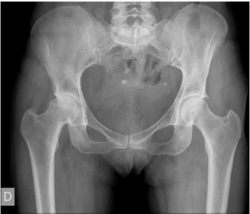
3.4 - X-ray Radiographs [27]

As mentioned in the introductory chapter, this image modality has frequent use, beingthe main image modality used in the orthopaedic field.

For this image modality, a series of excited photons are projected onto the patient’s body by an X-ray generator. These photons can then either be interact with tissue or pass through it. In either instance, its result is captured by an X-ray detector placed on the other side of the body portion aimed to be evaluated.

A photon can interact with matter in several forms. The predominant three interactions are the photoelectric absorption, Compton scattering and Rayleigh scattering. In the first interaction, the photon’s energy is absorbed by an electron leading to its ejection with or without kinetic energy depending on the energy absorbed. Compton scattering occurs if the photon’s energy is well above the ionization energy required for an electron to be removed from an atom. In this case, only part of that energy is transferred to an electron while the photon remains with energy following a different direction. Lastly, regarding Rayleigh scattering, despite having a low energy interaction, this interaction is still significant when it comes to lower energy scans, such as mammograms. In it, a photon is absorbed by an atom and is immediately released with the same energy but with different direction.

These interactions cause the photons to lose their energy which is in store absorbed by the tissue, creating the contrast in the image. However, being an ionizing radiation it is quite harmful for living tissue, with radiation overexposure being linked to the appearance of cancerous tumours, with the World Health Organization classifying X-rays as carcinogen [16].

Since bone has a high amount of calcium, which is a high atomic number atom, bones easily absorb X-ray waves, which makes them stand out from remaining tissues in this image modality, also making it perfect to use in an orthopaedic environment. The result of a projectional radiograph can be seen in figure 3.3, in which the bone clearly stands out from the remaining tissue.

Figure 3.3 – Hip X-ray radiograph displaying bone in a much brighter colour than its surrounding tissue

Chapter 4

Image Segmentation

4.1 - Introduction

Image segmentation is one of the primary steps in to build a patient-specific finite element model of a bone. After performing image acquisition, the segmentation step allows for the creation of an accurate geometric model of the bone domain, femur in this particular instance. In this chapter, an overview of segmentation techniques applied to different fields and image modalities previously delineated will be presented, increasingly funnelling to the situation at hand. A special focus will be given to techniques that apply to femur using radiographs.

4.2 - General overview

With the evolution of computer-aided diagnosis — CAD — and overall technologic influence in medicine, image segmentation has shown to be a crucial stage and has gained great advances in its medical application, especially in the last 30 years with the improvement of the several image modalities.

Several articles mark significant advances in medical image segmentation. Vincent et al. [28] first introduced, in 1991, the watershed method for image segmentation, practice which is now commonly used in image segmentation of different modalities. Another example is given to us by Yezzi et al. [29] who implemented active shape models, commonly known as snakes, to medical images and that method attracted the attention of the research community, having at least 262 paper citations, according to IEEE.

Despite the examples presented having applicability across multiple modalities, in some situations it is better to accommodate the segmentation method to the image modality in question. Noble and Boukerroui [30] presented an influent review paper on image segmentation methods on ultrasound. Despite presenting some methods that either could be generalised to different modalities, such as Chalana and Kim’s [31] and Mitchell et al.’s [32] techniques, most methods are specific to ultrasound and its applications. Considering cardiac ultrasound, Friedland and Adam [33] presented a pioneering work allowing the detection of cavity boundaries using simulated annealing, which is an optimisation algorithm with a Markovian spatio-temporal regularisation. At the same time, Mulet-Parada and Noble [34] proposed a local-phase-based approach to spatio-temporal endocardial border detection, arguing that local phase is a better basis for ultrasound-based feature detection and segmentation because local

Image Segmentation 18

18

phase is theoretically invariant to intensity magnitude. Alternatively, if breast cancer is considered, the work developed by Stavros et al. [35] greatly influenced the design of algorithms for breast mass detection as is seen in later publications, such as Drukker et al. [36], where mass detection is performed by first filtering the images with a radial gradient index filtering technique and, with it, thresholding occurs to delineate lesions.

When the focus is shifted to femur, several segmentation techniques can be found with high-end imaging techniques. Yan Kang et al. [37] suggested an adaptive region-growing method for femur segmentation on CT scans. Following the first region-growing step, some adjustments were performed in order to obtain a closed and smooth boundary. Along with this work, several others were based on CT scans to obtain a femur model, such as Saha and Wehril [38], who used a fuzzy distance transform based thickness to segment a femur, and Kaus et al. [39], who used a priori knowledge to build a 3D point distribution model of a femur.

For this work 2D radiographs will be used, therefore looking for segmentation methods that are adapted to that reality is vital.

4.3 - 2D x-ray segmentation techniques

As previously mentioned, X-ray is a frequently used image modality, but of which few segmentation methods exist in literature. To gather information on diverse methodologies required an extensive search activity, whose epitome will now be presented.

Baka et al. [40] presented a reconstruction of the distal femur using a statistical-shape model. In it, they use CT scans as training data to build an average point distribution 3D femur model. For each radiograph, the 3D model is projected in two dimensions, and using Canny edge detection, the model’s landmarks are adapted to the nearest edge. For each projected landmark, the 3D distance and angle is calculated between the 2D edge point and the original 3D landmark point. These two values become part of the energy value, and it is precisely this value which the method aims to minimize. To calculate it, the authors use the equation represented in (4.1), in which 𝑢𝑖(𝑝𝑗) serves as a mask for points that fall on projection 𝑖 or not,

𝑤𝑖(𝑝𝑗) determines the orientation weighing term, which is equal to cos (𝛼) for every calculated

angle below 90º, and, lastly, 𝐷𝑖(𝑝𝑗) establishes the distance term. Its calculation is visible in

equation (4.2), where 𝑣 controls the smoothness of the exponential. An overview of this method is seen on figure 4.1.

Θ

(𝑝

) = 1 − 𝑢

(𝑝

) ∗ 𝑤

(𝑝

) ∗ 𝐷

(𝑝

)

𝐷

(𝑝

) = exp (−

𝑑

(𝑝

)

𝑣

)

19 Image Segmentation

19

Figure 4.1 [40] - Overview of the steps taken to generate the model and calculate its energy value

Since a database of CT scans is not available, it is not possible to replicate this method. However, some techniques such as the Canny edge detection show great usefulness in the attainment of a 2D femoral model.

Bandyopadhyay et al. [41], more recently, presented an approach for long-bone fracture detection, tested on femoral bones, in which the segmentation is a pivotal initial step. In this study, the authors, after studying different segmentation methods opted to select an entropy-based algorithm. With it, local entropy is calculated in a 9x9 window, and in the biggest transitions the largest entropy should be identified due to varied local intensities. The outcome can be seen in figure 4.2. From this pre-processed image, the contour generation is done by using adaptive thresholding in an 8-neighbouring window. If a pixel has a value higher than the

Image Segmentation 20

20

adaptive threshold suggested, it will be part of the contour. This final contour is exemplified in figure 4.2.

Figure 4.2 [41] - (a) Original digital x-ray of broken femur, (b) pre-processing using local entropy computation and (c) contour generation based on the image obtained in (b)

To correct the contour obtained, the authors introduce a method they named relaxed digital straight line segments — RDSS. In this approach, Bandyopadhyay et al. [41] use chain code to characterize a close-ended digital curve and define 2 properties it must follow:

• R1 - The runs have at most two directions, differing by 45º.

• R2 - Both directions can have at-most three run lengths, which are consecutive integers.

By applying these properties to the contour, they create a simplified version of the generated contour. After using this technique, the algorithm is able to amend any discontinuities present due to the parallel property in consecutive line segment. The final result is seen in figure 4.3.

Figure 4.3 [41] - (a) Generated contour with discontinuities at A and B, (b) contour with RDSS applied and (c) contour with RDSS and no discontinuities

21 Image Segmentation

21

This work has a closer proximity to the conditions of the work to be developed and therefore, a lot more information can be recovered and used in the future.

One last work with high relevance is the one developed by Chen et al. [42]. In this work, Chen et al. present a method for segmenting the femur from hip x-rays with access to a set of training data. To do this, the authors try to identify three features: the femoral shaft, the femoral head and the turning point at the great trochanter. For each feature, they retrieve several candidates, which later on will be selected by the best fit. For the femoral shaft, the horizontal gradient is measured and scanned horizontally. The regions with a local maximum horizontal gradient will be selected as possible borders of the femoral shaft. The contour following method allows for the generation of each line. After obtaining several line candidates, the lines are paired by having the width closest to the training sample. For each pair of lines a probability value is attributed following the equation in (4.3), in which 𝑃𝑖 is the probability

value, 𝑀𝑖is the mean intensity gradient magnitudealong the line and 𝐺(𝑤𝑖| 𝜇, 𝜎) is the Gaussian

of the width 𝑤𝑖 in a distribution with 𝜇 average and 𝜎 standard deviation.

𝑃

= 𝑀

∙ 𝐺(𝑤

| 𝜇, 𝜎)

The pair of lines with the highest probability value is selected. For the femoral head, the vertical and horizontal gradients are computed, since the femoral head has a round shape both gradients should have a high value. From the top left region, a circular Hough transform is fitted over the points with higher gradient to obtain circles shaping the femoral head. To fit the best candidate, a different probability value is calculated through equation (4.4), in which it equals to the Gaussian of the ratio between each candidate radius and the width of the previously selected shaft.

𝑃

= 𝐺(𝑟

/𝑤| 𝜇, 𝜎)

In order to detect the turning point at the great trochanter, the femoral shaft outside border is extended upward continuing the border using the contour following method. After this, the second derivative is computed and the point with the highest second derivative is defined. In figure 4.4, a representation of this method applied to a single radiograph is presented.

Image Segmentation 22

22

Figure 4.4 [42] – (a) Candidate femoral shafts, (b) candidate femoral heads and (c) turning point (white point) at the great trochanter

After these features are extracted, an average model generated from the training samples is superimposed in the image. With it, a piecewise registration is performed. Using the features obtained above, the average model selects five feature points: the most top and the most left point in the femoral head border, the turning point, and the bottom two points in the femoral shaft. The piecewise registration is calculated according to equation (4.5), in which 𝒒 represents the image feature point, 𝒑 represents the model’s feature point, 𝑠 represents a scaling factor, 𝑹 represents a rotation matrix and, lastly,

𝑻

𝒒 = 𝑠 𝑹 𝒑 + 𝑻

As the last step, in order to adapt the model to each individual femur, an active contour, commonly known as snakes, is applied. This better adjusts the model to the image at hand, as it is visible in figure 4.5.

Figure 4.5 [42] – (a) Model femur contour divided into five segments, (b) piecewise registered femur model used as the initial configuration of the snake algorithm and (c) Extracted femur contour after

23 Image Segmentation

23

This work proposed in 2005 [41] has great relevance for the work to be developed here since both have similar conditions. The geometric approach to the femur segmentation seems adequate, since this particular bone has several unique geometric features, which, as it is perceptible in Chen et al.’s work, can be exploited to benefit this work.

From the work developed by Chen et al. [41], a lot was used. The use of the vertical and horizontal gradients was applied further on to the detection of femoral borders which allowed for the creation of a computational model.

Image Segmentation 24

Chapter 5

Finite Element Method

5.1 - Origins

Finite element analysis has its origins in 1940’s. With the emergence of digital computation, a conceptual approach to finite element analysis arose with Courant’s article [43]. However to put it in practice was a long and shared effort, that culminated in the paper written by Turner, Clough, Martin, and Topp [44], henceforth known as TCMT, in which the term finite element analysis was first coined. This method has great utility since it allows for modelling and discretization of several physical phenomena and history showed its eclectic application range. FEA was firstly used in physics in 1957 [45], however its big leap was when Argyris published a book on the use of FEM in aerospace engineering [46]. This development of finite element analysis was a consequence of a combination of several ingredients, one of which was digital computing. This technology was only affordable to this industry through mainframe computers [47].

From this start, the application of FEM began to branch out to several different fields. The piecewise analysis allowed it to be applied to fluid mechanics, electromagnetic fields and thermal and mass transport analysis [48], but most importantly the strain and stress analysis was applied in orthopaedics, starting in the early 1970’s [49].

5.2 - Formulation [50]–[52]

The FEM is characterized for modelling complex situations in discrete equations and points. From those defined solutions it is possible to interpolate any given point and obtain the chosen property. Therefore, this method allows for the accurate approximation, depending on the elements and the number of elements chosen, of a set of differential equations into discrete equation system in a finite number of points.

When FEA is applied to solid mechanics there are 4 main steps to follow: • Mesh creation, and the elements forming it

Finite Element Method 26

26

• Assembly, where the element-specific equations are combined • Boundary conditions and external forces applications

After these steps are followed, the equations can be obtained for strain and stress, which are, in our case, the desired results.

For the first step, the physical domain is divided into elements, which are in turn interconnected through their nodes. The aggregate of the different elements and its nodes constitutes a mesh. In order to obtain a representative model of the chosen object, one must divide it into a certain number of elements (for orthopaedic members is usually of the order of thousands) while considering its computational costs.

The second stage of the finite element method requires that, for each element, the shape functions are defined. These shape functions should describe the element’s behaviour and its variation across its structure and nodes.

Taking into consideration a determined 𝑢 function, it can be represented through an approximated function 𝑢ℎ. This function will be defined as a linear combination of basic

functions.

𝑢 ≃ 𝑢

𝑢

= ∑ 𝑢

𝜓

𝜓𝑖 represents the basic functions and 𝑢𝑖 the coefficients that approximate 𝑢ℎ to 𝑢. Figure

5.1 illustrates a 1D representation of the approximation of the 𝑢 function. At any given point, the 𝑢ℎ function defined through the sum 𝜓𝑖 × 𝑢𝑖, as defined in equation (5.2). The basic

functions will define how much impact a coefficient will have in determining the 𝑢ℎ function

throughout the element. In the case described in figure 5.1, 𝜓𝑖 is defined as linear basic

functions where its value is 1 for the respective node and 0 in every other node. This is true for any shape function as well, what can alter are the values between the nodes. In figure 5.1, it is possible to observe how the problem can be represented if the nodes are uniformly distributed or not. An irregular node distribution can be applicable in cases where 𝑢 has a greater variation, so it remains better represented in the 𝑢ℎ approximation.

Figure 5.1 [53] - The function 𝑢, solid line blue, is approximated by 𝑢ℎ, dotted red line, which is

calculated through a linear combination of 𝜓𝑖 linear basis functions and the 𝑢𝑖 coefficients. In the left a

27 Finite Element Method

27

Considering a 2D finite element with 𝑛 number of nodes, a vector of nodal displacements (in a 2D representation) is defined by:

{𝛿

_{} = {𝑢}

1

𝑣

𝑢

𝑣

… 𝑢

𝑣

}

𝑢 = ∑ 𝑁

𝑢

𝑣 = ∑ 𝑁

𝑣

In a solid mechanics FEA problem the displacements caused by the applied loads are unknown. The known variables are the body geometry, the physical parameters and the applied loads, which in turn are transformed in forces applied to the nodes. To obtain the nodal displacements caused from these nodal forces, a relationship between them should be defined taking into account the geometry and the physical characteristics of the body. For each element, the potential energy state can be represented as 𝜋𝑒 and its computation is

represented in equation (5.5).

𝜋

=

1

2

∫ [𝛿

]

_[𝑩]

_𝑫𝑩𝛿

𝑑𝑉

− ∫ [𝛿

]

[𝑵]

𝒑 𝑑𝑉

− ∫ [𝛿

]

[𝑵]

𝒒 𝑑𝑆

In equation (5.5), 𝛿𝑒 represents the element’s nodal displacements, 𝑵 the shape functions,

𝒑 the body forces per unit volume and 𝒒 the applied surface tractions. Other unexplained variables will be explored in detail afterwards. For a system in equilibrium, the potential energy is minimum. To reach this minimum, the derivative of equation (5.5) in respect to the element’s displacements, equation (5.6), should be equal to 0.

𝜕𝜋

𝜕𝛿

= ∫ ([𝑩]

𝑫𝑩)𝛿

𝑑𝑉

− ∫ [𝑵]

_{𝒑 𝑑𝑉}

− ∫ [𝑵]

_{𝒒 𝑑𝑆}

This equation can be rewritten in a simpler manner when it is equated to 0, as is seen in equation (5.7).

𝑭

_{= 𝑲}

_𝛿

𝑭𝑒_{represents the external forces applied in the nodes of the element, equation (5.8), and}

𝑲𝑒 _{denotes the element’s stiffness matrix.}

𝑭

= ∫ [𝑵]

𝒑 𝑑𝑉

𝑉𝑒

− ∫ [𝑵]

𝒒 𝑑𝑆

𝑆𝑒

Finite Element Method 28

28

Having the nodal forces 𝑭𝑒 _{determined as part of the conditions for the considered problem,}

it is still necessary to define the stiffness matrix of the element. It can be calculated through equation (5.9).

𝑲

= ∫ [𝑩]

𝑫𝑩𝑑𝑉

𝑉

(5.9)

The stiffness matrix depends on two factors: one physical and other geometrical. The physical factors of the elements are introduced in the 𝑫 matrix. This matrix is characterised by a 3 × 3 matrix, for 3D plane stress assumptions, that correlates local stresses with local strains through the Young’s modulus(𝐸) and the Poisson’s coefficient (𝑣). Both of these physical quantities are independent and experimentally obtained and depend solely of the material and its mechanical properties. To calculate the 𝑫 matrix the equation (5.10) is used, applied for plane strain:

𝑫 =

[

(1 − 𝑣)𝐸

(1 + 𝑣)(1 − 2𝑣)

𝑣𝐸

(1 + 𝑣)(1 − 2𝑣)

0

𝑣𝐸

(1 + 𝑣)(1 − 2𝑣)

(1 − 𝑣)𝐸

(1 + 𝑣)(1 − 2𝑣)

0

0

0

𝐸

2(1 + 𝑣)]

The 𝑩 matrix incorporates the geometrical factors. This matrix relates the element’s deformation with its nodal displacements. The calculation relies upon the shape functions 𝑁𝑖.

This matrix will differ in size depending on the amount of nodes that the element has, having a 3 × 2𝑛 size, considering a 2D element and 𝑛 number of nodes. This matrix can be calculated through equation (5.11).

𝑩 =

[

𝜕𝑁

𝜕𝑥

0

0

𝑑𝑁

𝑑𝑦

𝑑𝑁

𝑑𝑦

𝜕𝑁

𝜕𝑥

|

|

]

As seen in equation (5.9), the FEM requires a volume integral. Depending on the element chosen this can be of varied levels of difficulty. For a linear element, the estimation of the integral should easily feasible. However, for a more complex element with curve lines, for example, the computation of the volume integral can become of severe difficulty. To ease this step, isoparametric elements are usually applied by defining the element in natural coordinates. The natural coordinate system is defined according to the element’s geometry, making it simpler to work with the volume integral. Since the natural coordinates system do not vary according to the Cartesian geometry of the element, the element in its natural

29 Finite Element Method

29

coordinates will be represented in the same way regardless of its Cartesian geometry. In figure 5.2, a representation of the transformation of an element is presented in its natural coordinates.

Figure 5.2 - Linear and quadratic elements represented in their Cartesian coordinates with the natural coordinates system superimposed over it and, in the right, the representation of both elements in their

natural coordinates.

After the element is represented in its natural coordinates, it is necessary to define the shape functions according to this system. The way the shape functions are defined depends on the number of element nodes. Considering the example displayed in figure 5.2, the shape functions for a 4 node element can be define through equation (5.12) for all nodes, and the shape functions for an 8 node element can be defined through equations (5.13.1) to (5.13.3), considering that

𝜉

𝑁𝑖 =

1

4

(1 +

𝜉

)(1 +

𝜂

)

𝑁𝑖 =

1

4

(1 + 𝜉)(1 + 𝜂) −

1

4

(1 − 𝜉

_{)(1 + 𝜂) −}

1

4

(1 + 𝜉)(1 − 𝜂

_),

𝑖 = 1, 3, 5, 7

𝑁𝑖 =

1

2

(1 − 𝜉

_{)(1 + 𝜂),}

_{𝑖 = 2, 6}

𝑁𝑖 =

1

2

(1 + 𝜉)(1 − 𝜂

_),

_{𝑖 = 4, 8}

Consequently, the elements of the 𝑩 matrix, which have to be obtained through derivatives of the Cartesian coordinates, can be obtained from the natural coordinates following equation (5.14).

{

𝜕𝑁𝑖

𝜕𝑥

𝜕𝑁𝑖

𝜕𝑦 }

= [𝑱]

{

𝜕𝑁𝑖

𝜕

𝜉

𝜕𝑁𝑖

𝜕

𝜂

}

The Jacobian matrix is defined by the equation (5.15), however, another way of obtaining it, through the data available is using equation (5.16).