Impact of leverage in mergers & acquisitions performance : evidence from US public firms

(1)

Impact of Leverage in Mergers &

Acquisitions Performance: Evidence

from US Public Firms

Manuel Murta Cardoso

152418067

Dissertation written under the supervision of

Professor Diana Bonfim

Dissertation submitted in partial fulfilment of requirements for the MSc in

Finance, at the Universidade Católica Portuguesa

(2)

(3)

Impact of Leverage in Mergers & Acquisitions Performance: Evidence from US Public Firms

Manuel Murta Cardoso 152418067

Abstract:

The impact of leverage on post-merger performance has been a subject of relative low debate within the literature on Mergers & Acquisitions. Some authors have studied the impact of several variables in post-merger performance, such as methods of payment, prior M&A experience, and whether an acquisition was performed by a conglomerate. Nevertheless, there is a dearth of literature for exploring the impact of leverage on a firm’s post-merger performance. Thus, through the use of an innovative model, this dissertation studies the impact of the capital structure of the acquiring and targeted firm on the years following the merger. Based on a sample of 594 mergers between 1990 and 2013, we found that, on average, a highly leveraged firm acquiring either a highly leveraged company or a lowly leveraged firm was negatively and significantly associated with post-merger performance. We subjected our results to further testing through a specific analysis of recession and expansion years, against different risk categories of sample cases. Our results for these only further solidified the conclusions derived from our general sample analysis. This work has led to the conclusion that when acquiring firms are highly levered, the firm’s post-merger performance is weaker than otherwise.

Keywords: mergers, acquisitions, leverage, merger, performance

(4)

Impacto de Alavancagem no Desempenho de Fusões & Aquisições: Evidência de Empresas Públicas dos Estados Unidos da América

Manuel Murta Cardoso 152418067

Resumo:

O impacto da alavancagem no desempenho pós-fusão tem sido alvo de debate relativamente baixo na literatura sobre Fusões e Aquisições. Alguns autores estudaram o impacto de várias variáveis no desempenho pós-fusão, como métodos de pagamento, experiência anterior em Fusões e Aquisições e se uma aquisição foi realizada por um conglomerado. No entanto, existe escassez de literatura que explora o impacto da alavancagem no desempenho pós-fusão de uma empresa. Assim, através do uso de um modelo inovador, esta tese estuda o impacto da estrutura de capital da empresa adquirente nos anos subsequentes à fusão. Com base numa amostra de 594 fusões entre 1990 e 2013, descobrimos que, em média, uma empresa altamente alavancada que adquire uma empresa altamente alavancada ou uma empresa pouco alavancada está negativa e significativamente associada com o desempenho pós-fusão. Aplicámos a análise para anos de recessão e expansão e para diferentes categorias de risco. Os nossos resultados para estes apenas solidificaram ainda mais as conclusões derivadas da nossa análise geral da amostra. Esta tese levou à conclusão de que, empresas adquirentes altamente alavancadas, o desempenho pós-fusão da empresa é mais fraco do que o contrário.

Palavras-chave: fusões, aquisições, alavancagem, desempenho

(5)

(6)

Acknowledgements

First of all, I would like to convey my gratefulness to Professor Diana for her invaluable insights in Empirical Corporate Finance. Her guidance and advice were striking in developing this dissertation. Her support and availability were crucial to thriving during this semester. Her inspiration and encouragement were essential to conclude this journey. Therefore, without her, this dissertation would be much harder to complete. For that, I thank Professor Diana.

Secondly, to my colleagues, namely Joana Gomes, Carolina Viana, Francisco Lampreia, Diogo Macedo, José Amaral, Luís Frade, Carlota Galhardas, Catarina Silva and José Rodrigues, I thank them for their constant support during this last year. Their points of view and understandings helped me to succeed during this master’s degree.

Lastly but not least, I express my thankfulness to my parents for their sacrifice and commitment. To my brothers João and Miguel, who gave me remarkable perceptions about real-world applications of Finance and Management, I could not be more grateful.

Lisbon, January 2020 Manuel Murta Cardoso

(7)

(8)

I. List of Tables

Table 1 - Sample distribution by Years ... 16

Table 2 - Sample Distribution by Industry ... 17

Table 3 - Summary Statistics... 18

Table 4 - Annual firm median operating pre-tax cash flow return on assets in the years surrounding the merger ... 20

Table 5 - OLS Regressions where dependent variable corresponds to the variation between performance after and before the merger (absolute variation) ... 21

Table 6 - OLS Regressions where dependent variable corresponds to variation between performance after and before the merger (dummy variable) ... 23

Table 7- OLS Regressions for Recession Years (1990, 2001 and 2008) ... 25

Table 8 - OLS Regressions for Expansion Years ... 27

Table 9- OLS Regressions for Altman Z-score above the median of sample ... 29

(10)

2

II. Table of Figures

(11)

3

III. List of Abbreviations

D/A – debt over assets

H_H – highly levered acquiring a highly levered company H_L – highly levered acquiring a lowly levered company L_H – lowly levered acquiring a highly levered company L_L – lowly levered acquiring a lowly levered company LBO – leveraged buyout

M&A – mergers and acquisitions LBO – leveraged buyout

(12)

4

1. Introduction

Scholars have studied the impact of several variables on firms’ post-merger performances. Most of the literature, embodying the classical approach for assessing the post-merger performance of a firm, focuses on analysing abnormal returns around announcement dates. (Franks et al., 1991) However, a select few have studied merger performance from a long-term perspective. Historically, the literature has focused on variables such as methods of payment (DeAngelo et al., 1984; Travlos, 1987; Heron and Lie, 2002), prior M&A experience (Lahey and Conn, 1990; Bruton et al., 1994; Haleblian and Finkelstein, 1999) and whether an acquisition was performed by a conglomerate firm or not (Levy and Sarnat, 1970; Lewellen, 1971; Stein, 1997). The study of the capital structure of acquiring and target firms has been an overlooked variable in this context. Even though Smith (1990) studied the impact of leverage in securities prices and Heron and Lie (2002) analyse the impact of leverage on methods of payment, both sets of authors have fallen short of exploring the impact of leverage from both the acquiring and targeted firm on post-merger performance. Thus, our main objective in this dissertation is to focus on how firms’ capital structure might impact such post-merger performances.

Our innovative model studies the relationship between the capital structure of the companies involved in these transactions and the post-merger performance of the acquiring firm. For this purpose, we have divided our analysis into three main timeframes so as to capture any potential time-variant effects. Firstly, we consider the performance of both firms during the five years before and after the merger. Secondly, we perform the same analysis on the three years before and following the merger. Finally, we repeat these analyses solely on the one year before and the one year following the merger.

To assess the performance of the company, a particularly relevant measure suggested by Healy et al. (1992) is used. His work provides for the creation of a variable by dividing a firm’s pre-tax operating cash flow by the market value of its assets. The relevance of this measure is related with its proficiency in comparing performance across firms in a standardized manner. Since pre-tax operating cash flow over the market value of assets, an unlevered measure, excludes the effect of interests and taxes, the effect of the method of payment in earnings, which is a levered accounting variable, can be excluded. In the specific cases where the merger is financed by debt, earnings would be impacted, creating a strong bias in the results. Our proposed model studies the impact of four scenarios in post-merger performance: a highly levered company acquiring a highly levered company, a lowly levered company acquiring a lowly levered

(13)

5 company, a highly levered company acquiring a lowly levered company, and a lowly levered company acquiring a highly levered company.

We find that a highly leveraged firm acquiring either a highly leveraged firm or a lowly leveraged firm was associated with a negative and significant impact on post-merger performance. Our findings and analyses are based on a sample of 594 mergers between 1990 and 2013. These results are verified when considering both a three- and one-year timeframe of analysis pre- and post-merger. When analysing along a five-year period before and after the transaction instead, we were unable to find significant results. This might be explained by the dilution of the leverage effect over a longer period of time.

We then performed this same statistical model specifically on economic expansion and recession years within the sample. When economic recession years were considered, no relationship between leverage and post-merger performance was discovered. In the case of economic expansion years however, we found that, on average, a highly leveraged firm acquiring a lowly leveraged firm was associated with a negative impact on post-merger performance.

Moreover, the same methodology was studied for different risk categories. For that, we proxied company risk profile as the measure suggested by Edward Altman (1968) – Altman Z-Score. We could not find significant results when the Altman Z-Score of the acquirer is higher than the median of our sample. On the other hand, when the Altman Z-Score was lower than the median of the sample, we found that on average, a highly leveraged company acquiring other highly leveraged firms was associated with a negative impact on performance. The latter of these results occurs for a three-year analysis of pre- and post-merger performance. Finally, when a one-year margin for performance is analysed, we found that a when a highly leveraged firm acquires a lowly leveraged company there is also an overall decrease in the firm’s performance.

According to authors such as Loughran & Vijh (1997), and Oler (2008), the analysis of past mergers and acquisitions activity has proven that post-merger performance is typically negative. On the other hand, however, high leverage used for acquisition purposes is usually expected to generate an increase in performance since it can reduce agency costs, creating additional pressure on managers to allocate resources to productive projects (Jensen and Meckling, 1976). Jensen (1986) further finds that leverage creates friction on managers to spend more energy and time for the purpose of assuring the merger’s success. When considering the

(14)

6 trade-off theory suggested by Modigliani and Miller (1963), there are costs and benefits to increasing debt. Debt might increase the risk of bankruptcy and debt servicing costs but added leverage might reduce agency costs while increase tax shields.

The ultimate goal of our analysis is to assess whether managers should take the capital structure of their firms and companies into consideration in determining whether they are willing to acquire, before any M&A activity has taken place.

The remainder of this dissertation proceeds as follows. Section 2 presents the literature review on the impact of several variables in mergers and acquisitions’ performance, along with the most relevant literature on the influence of capital structures on firms’ decision-making processes regarding M&A. Section 3 describes the methodology used and explains our variable construction and selection. Section 4 describes the sources for our data and presents summary statistics, while Section 5 analyses our subsequent results. Our work is thus concluded in Section 6, with references and appendices being available for further perusal in Sections 7 and 8, respectively.

(15)

7

2. Literature Review

Post-merger performance is by no means an unusual topic within the mergers and acquisitions’ field of research. The classical approach for assessing performance after a merger is to evaluate the firm’s stock in order to detect any abnormal gains or losses (Franks et al., 1991). Several studies in the literature focus on the impact of abnormal returns around the day of the merger’s announcement. However, few studies analyse the long-term performance of such deals. Only a handful of approaches have been put forward to assess post-merger performance (Dimson and Marsh, 1986; Lakonishok and Vermaelen, 1990; Franks et al., 1991; Healy et al., 1992; Agrawal et al., 1992). These studies will be the subject of this chapter, and their utility towards this paper’s objective will be made clear.

Healy et al. (1992) study post-merger performances using a sample data of the 50 largest mergers in the US between 1979 and 1983. He conceptualizes cash flow over the market value of assets as a performance measure and compares the five years before the merger, by adding accounting fundamentals of the merged firms in those years, with the subsequent five post-merger years. The authors find that performance decreases after the post-merger, except when he compares their performance with the overall industry, whereby he concludes that there is an increase in relative asset productivity. They also find that there is a consistent relationship between post-merger performance and abnormal stock returns after merger announcements, which they justify with post-merger cash flow increases. On the other hand, Agrawal et al. (1992) chose to focus on the variance in shareholders' wealth over the five post-merger years. In their seminal 1992 paper, they use a sample data of mergers between NYSE acquirers and NYSE/AMEX targets from 1955 to 1987. Adopting the abnormal return methodology proposed by Dimson and Marsh (1986) and Lakonishok and Vermaelen (1990), they find that shareholders of the acquiring firm suffer a statistically significant loss of about 10% during the five years after such deals. Their findings challenge the results of Franks et al. (1991), who concluded that the variance in returns after the merger was not significantly negative. Agrawal et al. (1992) justify the difference in the results they obtained as time-dependent effects of the dataset Franks et al. (1991) relied upon.

A growing body of literature has examined the impact of several variables in post-merger performance. Most of the research focuses on variables such as (i) the method of payment (cash vs stock), (ii) prior M&A experience, and (iii) whether an acquisition was performed by a conglomerate firm or not.

(16)

8 The method of payment impact on post-merger performance has been a subject of constant debate over the years. There is a signalling effect on the method of payment in mergers and acquisitions. Managers of the bidder firm prefer cash offers when they believe that the target firm is undervalued, while stock offers are preferred when they wish to share acquisition risks with the seller (DeAngelo et al., 1984). Consequently, the market reacts positively to cash offers and negatively to stock offers, thereby affecting stock returns. Travlos (1987), using an event-study method, found that acquirer stockholders suffer significant losses in pure stock offers but experience normal returns in cash offers. They used a data set of mergers between 1972 and 1981 retrieved from The Center for Research in Security Prices (CRSP). These results are consistent with the signalling of the payment method that challenges the conclusions of Healy et al. (1992), as the latter do not find a relation between the method of payment and abnormal stock returns observed post-merger. A difference in the data samples might explain this disparity – Healy et al. (1992) only use the 50 largest mergers in their sample period, perhaps too low a number to yield significant results. Travlos (1987), on the other hand, use 167 acquiring firms (sixty are relative to stock offer, one hundred are cash offers, and seven are combinations of stock and cash). Healy et al. (1992) further do not specify the type of offers in his dataset. Heron and Lie (2002) seemingly confirm Travlos (1987)’s finding that merged firms experience negative abnormal returns after merger announcements through a stock offer, while cash offers are usually accompanied by normal returns. Nevertheless, they further find that post-merger returns are both positive for the two types of method of payment, being significantly higher for cash offers. Thus, they conclude that “both the bidder’s returns and the combined firm’s returns suggest that announcement of cash acquisitions convey more favourable information than do announcements of stock returns” (Heron and Lie, 2002: 139).

Some authors have studied the impact of previous M&A experience in post-merger performances. On the one hand, some authors propose that prior acquisition experience has no relation to the performance of an acquisition (Lahey and Conn, 1990). On the other hand, various researchers conclude that previous M&A experience has high explanatory power in regard to post-merger performance. Using a dataset of 449 acquisitions that occurred between 1980 and 1992, Haleblian and Finkelstein (1999) conclude that when an acquisition is dissimilar to previous acquisitions, the acquisition experience led to a negative impact on performance. Yet, when the current acquisition is similar to the previous acquisition, there is a positive influence on the performance. Bruton et al. (1994) and Haleblian et al. (2006) share this notion, but while the former test the impact of previous M&A experience in acquisitions of financially

(17)

9 distressed firms, the latter test it on the U.S’s commercial banking industry. Both sets of authors conclude that managers tend to adapt their behaviours according to previous experience, leading to a positive impact in post-merger performances.

There is also a lack of consensus in the literature on whether an acquisition made by a conglomerate firm has an impact on the combined firm’s performance. Some authors investigate the benefits of a conglomerate merger by evaluating the market side of the operation (Hadlock et al., 1999). Such investigations conclude that investors are reticent regarding conglomerates since they believe that such firms are very complex, creating difficulties in performing accurate valuations. Other researchers focus on the cash flow side:

1. evaluating correlations and significance of different income streams within conglomerate firms (Levy, 1970);

2. studying upsides in the ability to afford higher debt capacity to increase tax shields (Lewellen, 1971);

3. analyzing efficiency increases in investment activities by boosting internal capital markets (Stein, 1997).

Overall, there is a vast literature that assesses the impact of this variable in the post-merger performance. While some authors focus on positive motivation, others find negative reasons to diversify in what becomes conglomerate mergers.

Even though there is a vast literature on some of the variables that may affect the performance of a merged firm, others are still relatively unexamined. One such overlooked variable is the difference in capital structure between the bidder and the target firm. Smith (1986) analyses the impact of increases in leverage ratio on security prices, though he did not consider differences between the two firms prior to the merger. Heron and Lie (2002) also study the impact of increases in leverage ratios, but they study their relationship to methods of payment instead. There is a gap in the literature comprised of the failure to compare the capital structure of both the acquirer and target firm.

The choice of capital structure, however, is by no means an overlooked topic in the finance literature. One of the first steps in this field of research was made by Modigliani and Miller (1958), proposing the irrelevance theorem. This proposition denotes that financial leverage does not impact a firm’s value, i.e., the way that firms finance themselves (debt vs equity) does not have an impact on the firm’s value. By increasing debt, because it is cheaper than equity, the

(18)

10 company will face a higher equity cost. Therefore, the benefits of raising debt will be offset by the upsurge in equity costs.

Since markets are not efficient and embody several imperfections, Modigliani and Miller (1963) revisited their previous work to consider this time the costs (such as agency costs and financial distress costs) and benefits of debt (such as tax shields), leading to the creation of the static trade-off theory.

The second big step in capital structures decisions theory was brought forward by Myers and Majluf (1984) through the pecking order theory. This theory considers adverse selection problems (sellers have information that the buyer does not have) and builds a hierarchy for minimizing costs associated with such problems. According to Myers and Majluf, firms prefer retained earnings, then debt, and, ultimately, equity for the purposes of funding investment opportunities. This theory is justified by the adverse market reaction that accompanies the announcement of seasoned equity issuance. Debt, on the other hand, comprises a lower information asymmetry and thus yields lower remuneration for investors.

The consequences of leverage on acquisitions are an ambiguous subject among researchers. Harrison et al. (2014), using a sample of 2,218 acquisitions from 1972 to 2005, found that the amount of leverage carried out in acquisitions has a positive impact on performance. Their results are consistent with previous research. Jensen and Meckling (1976) found that higher leverage reduces agency costs because managers are restricted from pursuing investment opportunities that might lead to lower returns. Jensen (1986) also further considered the pressure on management to pursue projects with higher returns, leading to the acquisition of companies with more assured profit returns. On the other hand, some authors focus on the downsides of leverage in acquisitions. Lin and Chang (2012) study the relationship between the amount of leverage and financial distress costs, stating that managers feel forced to pursue projects with lower risk, reducing the value maximization principle that they would consider if they could instead pursue projects with higher risk. Testing for two different time periods (1978-1982 and 1983-1987), Miller and Bromiley (1990) concluded that debt is accompanied by a higher risk, which negatively impacts the company’s post-merger performance.

This research has significant further importance due to leveraged buyouts (LBOs). This type of acquisition has given a great deal of attention in the literature, not only because of high returns that private equity funds experience, but also due to secure access to debt by such funds for pursuing all types of investments, which might impact the global economy in the future. A

(19)

11 leveraged buyout (LBO) is the acquisition of a company by another company through the use of high amounts of debt. Most of the time, bidder firms use target assets as collateral. Many authors agree that LBO occurrence creates a significant positive impact on a firm’s performance (Palepu, 1990; Smith, 1990; Smart and Waldfogel, 1994), though some conclude that the amount of leverage instead has no impact. For Palepu (1990), factors like change in the organizational structure are the main reason for LBO success. On the other hand, Reich (1989) and Long and Ravenscraft (1993) draw an opposing conclusion regarding leveraged buyouts. They conclude that debt payment schedules lead to firms cutting R&D expenditures, affecting the post-acquisition performance of the company.

For some specialists, it is challenging to assess the post-performance of a buyout due to earnings manipulation by managers (Wu, 1997; Chou et al., 2006). Using a sample data of 87 management buyouts, Wu (1997) finds that managers tend to manipulate earnings prior to the deal in order to present the market with a positive post-merger performance. Chou et al. (2005) also show that there is often manipulation of earnings before a reverse LBO (turning a company that was privatized by a leveraged buyout into a public company again), which positively impacts the stock performance after issuance.

As such, there is a gap within the literature that evaluates the post-merger performance. There is already some research on the study of the impact of several variables on such performances, but the impact of the capital structure of both the acquiring firm and the target firm is still missing scrutiny. Furthermore, most of the research on M&A focus on stock returns, and rarely considers firm-level performance, utilized in this research as pre-tax operating cash flow over the market value of assets.

(20)

12

3. Methodology and Variable Construction

3.1. Dependent Variable: Difference in performance before and after the merger

The dependent variable is built by comparing pre-merger performance with post-merger performance. This performance measure is computed by dividing the pre-tax operating cash-flow of a company to the market value of its assets (Healy et al., 1992). The pre-tax operating cash-flow is defined by sales, minus cost of goods sold, selling and administrative expenses, in addition to any non-cash expenses (depreciation, amortization and goodwill). The market value of assets is computed by adding the market value of equity to the book value of debt. This measure enables us to create a variable that is comparable across firms, a pre-tax operating cash flow over the market value of assets. Excluding the effect of interest expense/income and taxes further enables us to avoid a potential entry point for bias in our results. By using pre-tax operating cash flow instead of accounting income, we exclude post-acquisition accounting earnings, which may arise due to methods of payment for the merger (cash vs stock). If an acquisition is financed by debt, post-accounting numbers will be influenced by the amount raised and, consequently, result in lower performance. Therefore, since earnings mirror capital structure choices and not the economic performance of the company, we do not consider accounting earnings. Since we are studying the impact of capital structure on performance, this effect would be repeatedly accounted for in our model.

The performance measure was computed for the five years preceding and following the merger. For the previous five periods, the performance measure is computed by summing the cash flows of the acquiring and targeted firms and dividing it by the sum of the market value of the assets of both. Furthermore, post-merger performance is computed by dividing the cash flow of the acquiring firm by the market value of its assets. The median of the five years prior to the merger, and the five years following the merger can then be computed. This difference between both medians then corresponds to the dependent variable. If its value is positive, we can state that there was an increase in performance. However, if its value is negative, we should state that there was a decrease in performance. The same analysis was performed considering three- and one-year range before and after the merger.

3.2. Independent Variables: Leverage Dummies

To recap, the main objective of this analysis is to study the impact of leverage on both the target’s and acquiring company’s post-merger performances. Hence, in order to assess the difference between a highly leveraged and a lowly leveraged company, limits must be chosen.

(21)

13 Here we consider values above the median of leverage ratios of stand-alone companies as being highly leveraged, with values below the median of leverage ratios of stand-alone companies as being lowly leveraged. We are thus able to assess what kind of merger we are considering - a highly levered company acquiring a highly levered company, a lowly levered company acquiring a lowly levered company, a highly levered company acquiring a lowly levered company (and vice-versa). In this manner, three dummy variables were created for our purposes. For a clearer perception, figure 1 presents a simplified diagram with the four types of mergers.

Figure 1 - Types of Mergers according to Leverage Ratios

This variable construction method has some limitations that should be highlighted. Firstly, when considering observations above and below the median, we have undertaken the assumption that our sample contains both highly leveraged firms and lowly leveraged firms. Secondly, we consider that our sample is illustrative of M&A activity in the sample period. This might not occur due to the preliminary clearing from our dataset of any observations that did not have available accounting data for the relevant time periods.

3.3. Control Variables

In order to capture the effects of other variables on post-merger performance, further measures were added to the model. As such, we drew on the model proposed by Harrison (2014). Therefore, we used the following variables, all of which concern the year immediately preceding the merger:

Industry Variable: in order to capture industry-specific effects on the post-merger performance

(22)

14 creation of a dummy variable. This variable is assigned a value of 1 whenever both companies belonged to the same industry (most often in horizontal mergers), and a value of 0 otherwise (often the case in conglomerate mergers).

Cash and short-term investments: our variable, in this case, consists of cash and short

investments, scaled by total assets. This measure is considered for both the targeted and acquiring firms.

Acquirer Market-to-Book (M/B): this variable consists of the total book value of common

equity, divided by market capitalization. This measure is usually used as a proxy for a company’s future growth prospects (Fama and French, 1995; Penman, 1996; Frank and Goyal, 2009).

Acquirer Sales Growth: this variable is constructed by calculating the difference between

current yearly sales with previous yearly sales, dividing by prior year sales. This variable is usually used to gauge a firm’s growth at the operational level. (Gupta, 1969; Garlappi et al., 2008; Harrison, 2014)

Relative target size: computed by dividing the market capitalization of the target firm by the

acquiring firm’s market capitalization. This variable allows us to account for the effect of the target on the merged firm’s performance. (Harrison, 2014)

Acquirer Net Operating Assets: this measure follows on the footsteps of work done by Nissin

and Penman (2001). Our variable is constructed by the sum of net financial obligations with common equity, in addition to minority interests. Firstly, net financial obligations are defined as the difference between financial obligations and financial assets. Financial obligations are expressed as debt in current liabilities, along with total long-term debt, with preferred stock added, subtracting preferred stock in treasury, and further adding preferred dividends in arrears. Financial assets are composed of the sum of cash and short-term investments along with other investments in advances. Secondly, common equity is calculated by summing common equity and preferred stock in treasury, and subtracting preferred dividends in arrears. Finally, minority interests are retrieved from the financial statements of our firms. This variable is scaled by lagged total assets1.

Acquirer Accruals: this variable is constructed along the lines of Richardson et al.’s (2005)

work. It is computed by summing the change in working capital, in non-current operating

1 Variable is scaled by lagged total assets for the purpose of avoiding problems that might arise for

(23)

15 accruals, and in financial assets. This summed change corresponds to the variation from the prior year to the current year. Firstly, working capital is calculated by subtracting current operating liabilities from current operating assets. Current operating assets, in turn, is constructed by subtracting the difference between current assets and cash and short-term investments, while current operating liabilities are defined as current liabilities minus debt in current liabilities. Secondly, variation in non-current operating accruals is calculated by subtracting the difference between non-current operating assets and non-current operating liabilities. Non-current liabilities are themselves calculated as total assets minus current assets, while also subtracting other investments in advances. Non-current liabilities are totalled by subtracting current liabilities and long-term debt from total liabilities. Finally, change in financial assets is itself the difference between financial assets and financial liabilities. While financial assets are defined as the sum of short-term investments and other investments in advances, financial liabilities are instead calculated as total liabilities, plus debt in current liabilities, plus preferred stock. As Acquirer Net Operating Assets, this variable is scaled by lagged total assets.

Acquirer Altman Z-Score: this variable corresponds to the Altman z-score formula: Z-Score =

1.2A + 1.4B + 3.3C + 0.6D + 1.0E, where A = working capital / total assets, B = retained earnings / total assets, C = earnings before interest and tax / total assets, D = market value of equity / total liabilities and E = sales / total assets. This discriminant-ratio model, created by Altman (1968), allows us to predict corporate bankruptcy using accounting ratios. The higher the z-score, the lower the company’s probability of bankruptcy. When the score is higher than 3.0, bankruptcy is unlikely. If the score is below 1.8 however, there is a high likelihood of the company becoming bankrupt shortly. This variable is further explained with more detail in Section 5.

As such, the following regression will be estimated:

∆𝑃𝑒𝑟𝑓𝑜𝑟𝑚𝑎𝑛𝑐𝑒_𝑖= (𝐻 − 𝐻 𝐷𝑢𝑚𝑚𝑦)_𝑖+ (𝐿 − 𝐿 𝐷𝑢𝑚𝑚𝑦)_𝑖+ (𝐻 − 𝐿 𝐷𝑢𝑚𝑚𝑦)_𝑖+ 𝐴𝑐𝑞𝑢𝑖𝑟𝑒𝑟 𝐶𝑎𝑠ℎ_𝑖 + 𝑇𝑎𝑟𝑔𝑒𝑡 𝐶𝑎𝑠ℎ𝑖+ 𝐴𝑐𝑞𝑢𝑖𝑟𝑒𝑟 𝐵𝑜𝑜𝑘 𝑡𝑜 𝑀𝑎𝑟𝑘𝑒𝑡𝑖+ 𝐴𝑐𝑞𝑢𝑖𝑟𝑒𝑟 𝑆𝑎𝑙𝑒𝑠 𝐺𝑟𝑜𝑤𝑡ℎ 𝑖

+ 𝑅𝑒𝑙𝑎𝑡𝑖𝑣𝑒 𝑇𝑎𝑟𝑔𝑒𝑡 𝑆𝑖𝑧𝑒_𝑖+ 𝐴𝑐𝑞𝑢𝑖𝑟𝑒𝑟 𝑁𝑒𝑡 𝑂𝑝𝑒𝑟𝑎𝑡𝑖𝑛𝑔 𝐴𝑠𝑠𝑒𝑡𝑠_𝑖+ 𝐴𝑐𝑞𝑢𝑖𝑟𝑒𝑟 𝐴𝑐𝑐𝑟𝑢𝑎𝑙_𝑖 + 𝐴𝑐𝑞𝑢𝑖𝑟𝑒𝑟 𝐴𝑙𝑡𝑚𝑎𝑛 𝑍 − 𝑆𝑐𝑜𝑟𝑒 _𝑖+ 𝜖_𝑖

(24)

16

4. Data and Summary Statistics

Our research considers all completed mergers between 1990 and 2013 in which accounting data was available in Compustat North America for the previous and subsequent five years of the effective date of the merger. Furthermore, it only considers mergers between US public companies during the relevant time period, a requirement in order to have available data through Compustat. Moreover, our sample does not consider financial and utility companies, since they are subject to special accounting and regulatory requirements (Healy et al., 1992; Fama and French, 2002; Uysal, 2011). Therefore, using the Deal Screener by Thomson Reuters Eikon, we were able to retrieve our dataset sample, comprising 594 mergers between a total of 1188 firms.

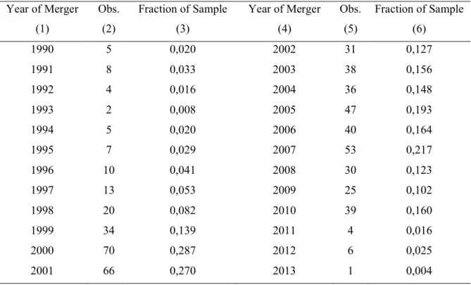
Table 1 - Sample distribution by Years

Table 1 presents the distribution of transactions by years. Columns (1) and (4) represent the year of the merger. Columns (2) and (5) correspond to the absolute number of deals considered in the sample. Concerning columns (3) and (6), they represent the relative fraction of mergers in the sample. It is computed by dividing the absolute value by the total number of observations. The sample comprises 594 transactions between 1990 and 2013.

Table 1 seen above explores the distribution of deals on a yearly basis. A visual analysis of the data allows us to develop some preliminary conclusions. Firstly, most of the deals in the sample take place between 1999 and 2010. Secondly, there is an increasing trend of deals between 1990

Year of Merger (1) Obs. (2) Fraction of Sample (3) Year of Merger (4) Obs. (5) Fraction of Sample (6) 1990 5 0,020 2002 31 0,127 1991 8 0,033 2003 38 0,156 1992 4 0,016 2004 36 0,148 1993 2 0,008 2005 47 0,193 1994 5 0,020 2006 40 0,164 1995 7 0,029 2007 53 0,217 1996 10 0,041 2008 30 0,123 1997 13 0,053 2009 25 0,102 1998 20 0,082 2010 39 0,160 1999 34 0,139 2011 4 0,016 2000 70 0,287 2012 6 0,025 2001 66 0,270 2013 1 0,004

(25)

17 and 2001, reaching its highest value in 2000, with 71 deals. Finally, at the beginning of the century, there is a marked deceleration in M&A activity, with the number of transactions consistently falling below a yearly total of 50. In fact, only 2007, the year prior to the financial crisis, saw a number of transactions higher than 50.

Our conclusions here have some limitations that must be highlighted. Firstly, the lack of deals in the first years of our sample can be explained by Compustat’s lack of information on individual companies’ fundamentals. Secondly, in the most recent years (between 2011 and 2013), the low amount of observations in the sample is explained by missing information about companies accounting data in pre or post-merger years. All in all, 744 observations were lost due to the lack of accounting data for the prior and posterior five years in both the acquirer and target company.

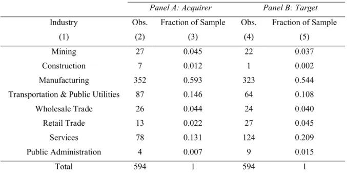
Table 2 - Sample Distribution by Industry

Table 2 presents the distribution of companies involved in transactions by industry. Panel A comprises data of the acquirer firm, while Panel B presents data of the target. In column (1) are represented the SIC industries. Columns (2) and (4) represent the number of companies in each industry for acquirer and target, respectively. Concerning columns (3) and (5), they represent the relative fraction of firms in the sample. It is computed by dividing the absolute value by the total number of observations in acquirer and target, respectively. The sample comprises 594 transactions between 1990 and 2013.

Table 2 allows us to visually inspect the distribution of companies by industry. Relative to all the companies in the sample (acquirers and targets), most firms belong to the Manufacturing

Panel A: Acquirer Panel B: Target

Industry (1) Obs. (2) Fraction of Sample (3) Obs. (4) Fraction of Sample (5) Mining 27 0.045 22 0.037 Construction 7 0.012 1 0.002 Manufacturing 352 0.593 323 0.544

Transportation & Public Utilities 87 0.146 64 0.108

Wholesale Trade 26 0.044 24 0.040

Retail Trade 13 0.022 27 0.045

Services 78 0.131 124 0.209

Public Administration 4 0.007 9 0.015

(26)

18 industry (approximately 59.3% in acquirers and 54.4% in targets). Therefore, our research results may be particularly relevant for the Manufacturing industry, in contrast with transactions involving the Construction and Public Administration industry, which represent a marginal part of the total sample. The second industry with the highest share in our sample is Transportation & Public Utilities, and Services, for acquiring and target firms, respectively.

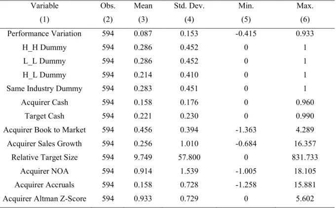
In order to describe the variables used in our model, Table 3 presents the summary statistics of our sample. In terms of our performance variation variable, we observe a variation between -0.415 and 0.933, effectively suggesting that there are companies within our sample where performance decreased by approximately 41.5 percentage points from the prior to the subsequent five years relative to the merger, while in others the performance measure increased by approximately 93.3 percentage points.

Table 3 - Summary Statistics

Table 3 reports the summary statistics for the variables used in the analysis. The variables, represented on column (1), are described through mean, standard deviation, minimum and maximum in columns (3), (4), (5) and (6), respectively. The number of observations is embodied in column (2). The sample comprises 594 transactions between 1990 and 2013.

Before presenting model estimates, we can further explore Appendix 1 to determine the correlation between the model variables. One can see that the correlation between dependent

Variable (1) Obs. (2) Mean (3) Std. Dev. (4) Min. (5) Max. (6) Performance Variation 594 0.087 0.153 -0.415 0.933 H_H Dummy 594 0.286 0.452 0 1 L_L Dummy 594 0.286 0.452 0 1 H_L Dummy 594 0.214 0.410 0 1

Same Industry Dummy 594 0.283 0.451 0 1

Acquirer Cash 594 0.158 0.176 0 0.960

Target Cash 594 0.221 0.230 0 0.990

Acquirer Book to Market 594 0.456 0.394 -1.363 4.289

Acquirer Sales Growth 594 0.256 1.010 -0.684 16.357

Relative Target Size 594 9.749 57.800 0 831.733

Acquirer NOA 594 0.914 1.539 -1.005 18.105

Acquirer Accruals 594 0.158 0.728 -1.258 15.881

(27)

19 variables and independent variables range between -0.106 and 0.119. However, the variables that embody the motivation behind the study (H_H, L_L and H_L) range between -0.059 and 0.045. If we analyse them individually, we can determine that a highly leveraged acquiring firm, buying a highly leveraged target firm, is associated with a negative performance ex-post. This result contrasts with a lowly levered company buying a lowly levered company and a highly levered company buying a lowly levered company. However, the latter is very close to zero, which leads us to expect that the coefficient should not be statistically significant should we run a regression analysis.

In order to better understand the distribution of performance measures, Table 4 (panel A) presents median pre-tax operating cash flow returns for merged firms between year -5 and -1. Panel B of table 4 reports the same measures for year 1 to 5. The medians of performance in years -5 to -1 range from 0.162 and 0.193 in our pre-merger years. In the post-merger context, medians varied between 0.251 and 0.267. When the median of annual performance for years -5 to -1 and 1 to 5 is calculated, the result is 0.177 and 0.261 respectively. Therefore, by subtracting post-merger performance from the pre-merger performance, we can see that on average, performance is higher. This challenges Healy et al.’s (1992) results, where they found that performance on average decreases. They justify their results by the absence of the impact of changes in equity due to overall market movements that may impact measurements over time. Furthermore, the authors relied solely on the 50 largest mergers between 1979 and 1983. This is a relatively low sample of observations and may be affected by external circumstances which were not discriminated or explored in their analysis.

(28)

20

Table 4 - Annual firm median operating pre-tax cash flow return on assets in the years surrounding the merger

Table 4 embodies the performance measures of firms in each year. The performance measure follows the definition of Healy et al. (1992). This performance measure is computed by dividing the pre-tax operating cash-flow of a company to the market value of its assets. The pre-tax operating cash-flow is defined by sales, minus cost of goods sold, selling and administrative expenses, in addition to any non-cash expenses (depreciation, amortization and goodwill). The market value of assets is computed by adding the market value of equity to the book value of debt. Pre- and pro-merger performance measures are respectively represented in panel A and panel B. In each panel, the median of performance for each year is represented. Posteriorly, the median of those five years is retrieved. Panel C represents the Median annual difference between performance in years -5 to -1 and 1 to 5. The sample comprises 594 transactions between 1990 and 2013.

Panel A: Pre-merger performance Panel B: Post-merger performance

Year relative to the merger (1)

Firm Median (2)

Year relative to the merger (3) Firm Median (4) -5 0,162 1 0,251 -4 0,165 2 0,261 -3 0,177 3 0,262 -2 0,189 4 0,267 -1 0,193 5 0,261

Median annual performance for

years - 5 to -1 0,177

Median annual performance for

years 1 to 5 0,261

Panel C: Difference between pre- and post-merger performance Median annual difference between

performance in years -5 to -1 and 1 to 5

(29)

21

5. Results and Empirical Analysis

5.1. Analysis of Capital Structure as Predictor of Post-Merger Performance

Following the explanation embodied in Section 3, Table 5 (Panel A) presents the estimation output of the OLS regression. The sample here relies on the difference between the medians of the five pre- and post-merger years as a dependent variable. We have also experimented with different time frames, reducing the margin to three years for Panel B, and down to one year for Panel C. The OLS estimators for control variables are presented in Appendix 2.

Table 5 - OLS Regressions where dependent variable corresponds to the variation between performance after and before the merger (absolute variation)

Table 5 represents the coefficients of the explanatory variables (without control variables) when the absolute variation of performance is considered. Panel A considers performance for a range of five years. Panel B represents coefficients for a range of three years. Panel C only reflects performance one year before and after the merger. H_H Dummy, L_L Dummy and H_L Dummy represent the explanatory variables. The sample comprises 594 transactions between 1990 and 2013. Robust standard errors are represented in parentheses. ***, **, * denote statistical significance at 1%, 5% and 10%, respectively.

Drawing from the regression presented in Panel A, one could conclude that none of the explanatory variables’ coefficients is statistically significant. A subsequent analysis of panel B and C, however, reveals some significance. Variable coefficients that are defined by a highly

Variables Panel A: Five Years Variation

Panel B: Three Years Variation

Panel C: One Year Variation Intercept 0.076*** 0.009*** 0.067*** (0.020) (0.024) (0.019) H_H Dummy -0.023 -0.043** -0.027* (0.018) (0.020) (0.017) L_L Dummy -0.012 -0.020 -0.025 (0.018) (0.020) (0.019) H_L Dummy -0.012 -0.038* -0.048*** (0.022) (0.023) (0.020) Observations 594 594 594 R-squared 0.065 0.051 0.048

(30)

22 levered company acquiring a highly levered company (H_H Dummy) and a highly levered company acquiring a lowly levered firm (H_L Dummy) are negative and statistically significant at the 5% and 10% significance levels in panel B. These are also negative and statistically significant at the 10% and 1% significance levels in panel C.

When we consider a range of five years for assessing the performance of a merger, our original time period is too extensive to demonstrate the impact of differences in leverage on such mergers. There are several other effects in the five pre- and post-merger years that might affect performance, such as management quality and the macroeconomic context during those years. These could dilute the effect of leverage in a firm’s performance. Such effects can explain why, when the time period is reduced to three and one years in our analysis, there is a clear correlation between leverage and post-merger performance.

When considering our three-year regression analysis (Panel B), our results suggest that in the case of both a highly levered firm acquiring a highly levered company, and a highly levered firm acquiring a lowly levered firm, a negative impact on performance should be expected. These results support Miller and Bromiley’s (1990) findings, who conclude that debt is accompanied by a higher risk which negatively impacts a company’s post-merger performance. Overall, one can see that, on average, carrying relative high levels of debt in the acquisition negatively impacts post-merger performance.

An analysis of panel C appears to confirm our panel B results. The performance of one pre- and post-merger year suggest once more that a highly levered firm acquiring a highly levered company, and a highly levered firm acquiring a lowly levered firm, are associated with a negative impact on performance. The specific coefficient results we get from panel B and C are significant at different significance levels, but they nevertheless support the same conclusion – when acquirers have highly levered capital structures, these results, on average, in a negative impact on performance.

Another way to assess the impact of leverage in performance within our model is to utilize performance variation as a dummy variable. This is in contrast to our previous use of the difference between performance ratios before and after the merger as a dependent variable. The performance measure corresponding to the years after the merger was built through the sum of pre-tax operating cash flows of the acquiring and target firm, divided by the sum of the market value of the assets of both firms. Furthermore, the performance measure representing the years immediately following the merger was calculated as the ratio between pre-tax operating cash

(31)

23 flow and the market value of the assets of the acquiring firm. The difference of both ratios corresponded to the performance variation in percentage points. If this difference was a positive value, it was considered in our analysis as a performance improvement. In cases where this value was negative instead, it could be concluded that there was a deterioration in overall performance.

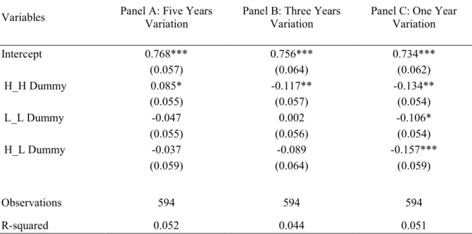
In table 6, the dependent variable is measured as a dummy variable. This variable took a value of 1 when there was an increase in performance (variation higher than 0) and a value of 0 where there was a negative variation (variation lower than 0), and consequently, a decrease in performance. Panel A follows the methodology described in Section 3, in which performance is built by taking a five-year timeframe into consideration, while Panels B and C are constructed on three- and one-year performance timeframes, respectively. The OLS estimators for control variables are represented in Appendix 3.

Table 6 - OLS Regressions where dependent variable corresponds to variation between performance after and before the merger (dummy variable)

Table 6 represents the coefficients of the explanatory variables (without control variables) when the variation of performance is considered. The dependent variable takes a dummy variable. Panel A considers performance for a range of five years. Panel B represents coefficients for a range of three years. Panel C only reflects performance one year before and after the merger. H_H Dummy, L_L Dummy and H_L Dummy represent the explanatory variables. The sample comprises 594 transactions between 1990 and 2013. Robust standard errors are represented in parentheses. ***, **, * denote statistical significance at 1%, 5% and 10%, respectively.

Panel C: One Year Variation Intercept 0.768*** 0.756*** 0.734*** (0.057) (0.064) (0.062) H_H Dummy 0.085* -0.117** -0.134** (0.055) (0.057) (0.054) L_L Dummy -0.047 0.002 -0.106* (0.055) (0.056) (0.054) H_L Dummy -0.037 -0.089 -0.157*** (0.059) (0.064) (0.059) Observations 594 594 594 R-squared 0.052 0.044 0.051

(32)

24 By analyzing the results of table 6 (Panel A), where we consider performance over a five-year period, it becomes evident that the H_H Dummy coefficient is statistically significant at the 10% significance level. The coefficient value itself is positive, which implies that a highly leveraged firm acquiring a highly leveraged company is, on average, associated with a positive impact on the merged firm’s performance. Several reasons can be put forward to explain this outcome. Firstly, companies with higher performance levels and, therefore, lower risk, may have higher debt capacity to pursue positive net present value projects. (Lewellen, 1971; Levy and Sarnat, 1970) Thus, when firms are able to raise debt to finance inorganic growth, this activity is likely to result in an improvement in overall performance. Secondly, these results support Servaes’s (1991) outcomes theory, in which he concludes that a high proportion of debt in an acquiring firm’s capital structure limits the management ability of misuse of cash flows, pursuing only projects with positive net present value. Finally, and according to Jensen’s free cash flow theory (1986), an overarching increasing cost of debt after debt raised for acquisition purposes creates added pressure on managers to be as efficient as possible.

The results we obtained in panel B and panel C, challenge the outcome of panel A’s five-year margin analysis. A straightforward reduction in the timeframe to three and one years leads to a considerable change in the value of our coefficients. In panels B and C, the H_H Dummy variable coefficient is negative at the 5% significance level. One of the possible reasons for this occurrence is that the impact of positive leverage in performance can only be accurately assessed in the long run, rather than in the short run. When the three- and one-year spans are considered, one can only observe the negative impact of debt in performance. When the time span under analysis is increased, the benefits of debt can be detected. In panel C, one can also see that the L_L Dummy variable coefficient is positive, which implies that in most cases, a lowly leveraged firm acquiring a lowly leveraged company is related to a decrease in performance. One of the more evident reasons for this result is the acquirer’s lack of ability to raise debt, due to the project’s high risk. Therefore, acquirers cannot achieve an improvement in operating performance through the acquisition. The H_L Dummy variable’s coefficient, on the other hand, is negative at the 1% significance level. This result directly supports the findings of Miller and Bromiley (1990), who conclude that debt implies higher risk, which in turn negatively impacts the company’s post-merger performance.

5.2. Expansion vs Recession Years Analysis

For further analysis, we increased the scope of our model to include expansion and recession years. This increase was motivated by the importance of the macroeconomic context on the

(33)

25 success of mergers and acquisitions, and therefore crucial to modelling a firm’s overall performance. For this purpose, we used the US Business Cycle Expansions and Contractions data provided by The National Bureau of Economic Research and studied by the Federal

Reserve Bank of St. Louis. Their data is composed of dummy variables which embody periods

of expansion and recession. According to their study, within our sample period, 1990, 2001, 2008 constituted periods of recession, while the remaining years were considered periods of expansion. The following regressions follow the methodology explained in section 3, where the absolute variation between pre- and post-merger years is considered.

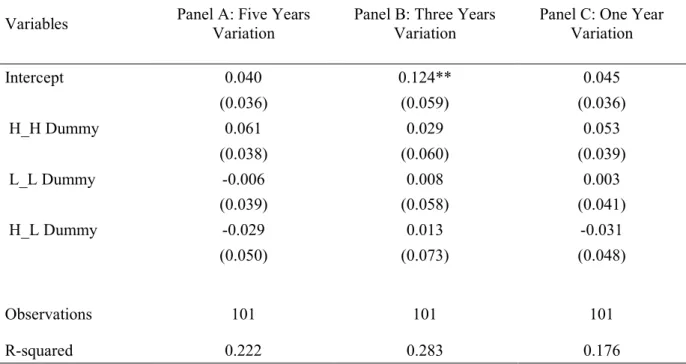
Table 7- OLS Regressions for Recession Years (1990, 2001 and 2008)

Table 7 represents the regression outputs when recession years are considered, excluding control variables coefficients. We used the US Business Cycle Expansions and Contractions data provided by The National Bureau of Economic Research and studied by the Federal

Reserve Bank of St. Louis. Panel A considers performance for a range of five years. Panel B

represents coefficients for a range of three years. Panel C only reflects performance one year before and after the merger. H_H Dummy, L_L Dummy and H_L Dummy represent the explanatory variables. The sample comprises 594 transactions between 1990 and 2013. Robust standard errors are represented in parentheses. ***, **, * denote statistical significance at 1%, 5% and 10%, respectively.

Table 7 provides us with the OLS coefficients for H_H Dummy, L_L Dummy and H_L Dummy variables. The OLS estimators for control variables are further provided in Appendix 4. While Variables Panel A: Five Years _Variation Panel B: Three Years _Variation Panel C: One Year _Variation

Intercept 0.040 0.124** 0.045 (0.036) (0.059) (0.036) H_H Dummy 0.061 0.029 0.053 (0.038) (0.060) (0.039) L_L Dummy -0.006 0.008 0.003 (0.039) (0.058) (0.041) H_L Dummy -0.029 0.013 -0.031 (0.050) (0.073) (0.048) Observations 101 101 101 R-squared 0.222 0.283 0.176

(34)

26 panel A follows the difference in the performance medians of the five pre- and post-merger years, panel B and panel C, consider three and one years, respectively. By analyzing our table 7 results, we find that none of the explanatory variables has significant coefficients for our three scenarios. A possible interpretation is that the low number of observations under analysis are insufficient to produce statistically significant results. When expansion periods are considered however, as evidenced by table 8 below, the H_L Dummy variable coefficient within our three-year analysis is statistically significant at the 10% significant level. The negative coefficient implies that, on average, a highly leveraged company acquiring a lowly levered firm, is associated with a negative impact on performance. These results offer support to our analysis in section 5.1, which is itself supportive of Miller and Bromiley (1990)’s work, on the relationship between leverage and risk and its negative impact on performance. The OLS estimators for our control variables are provided in Appendix 5.

(35)

27

Table 8 - OLS Regressions for Expansion Years

Table 8 represents the regression outputs when expansion years are considered, excluding control variables. We used the US Business Cycle Expansions and Contractions data provided by The National Bureau of Economic Research and studied by the Federal Reserve Bank of St. Louis. Panel A considers performance for a range of five years. Panel B represents coefficients for a range of three years. Panel C only reflects performance one year before and after the merger. H_H Dummy, L_L Dummy and H_L Dummy represent the explanatory variables. The sample comprises 594 transactions between 1990 and 2013. Robust standard errors are represented in parentheses. ***, **, * denote statistical significance at 1%, 5% and 10%, respectively.

5.3. Risk Categories Analysis

Edward Altman (1968) created a Z-score measure to predict the chance of a given company going bankrupt. This method of assessing bankruptcy probability of a company is inherently reliant on historical data. This data is extracted from companies’ financial statements. There are two extensions of this model, which can be dubbed as z’-score and z’’-score. This measure is, however, only applicable to privately held companies. Overall, this calculation of credit risk takes five ratios into account: profitability, leverage, liquidity, solvency and activity. The following formula provides an illustration of the Z-Score:

𝑍 − 𝑆𝑐𝑜𝑟𝑒 = 1.2𝑊𝑜𝑟𝑘𝑖𝑛𝑔 𝐶𝑎𝑝𝑖𝑡𝑎𝑙 𝑇𝑜𝑡𝑎𝑙 𝐴𝑠𝑠𝑒𝑡𝑠 + 1.4 𝑅𝑒𝑡𝑎𝑖𝑛𝑒𝑑 𝐸𝑎𝑟𝑛𝑖𝑛𝑔𝑠 𝑇𝑜𝑡𝑎𝑙 𝐴𝑠𝑠𝑒𝑡𝑠 + 3.3 𝐸𝐵𝐼𝑇𝐴 𝑇𝑜𝑡𝑎𝑙𝐴𝑠𝑠𝑒𝑡𝑠+ 0.6 𝑀𝑉 𝐸𝑞𝑢𝑖𝑡𝑦 𝐵𝑉 𝐿𝑖𝑎𝑏𝑖𝑙𝑖𝑡𝑖𝑒𝑠+ 0.99 𝑆𝑎𝑙𝑒𝑠 𝑇𝑜𝑡𝑎𝑙 𝐴𝑠𝑠𝑒𝑡𝑠 ,

Panel C: One Year Variation Intercept 0.067*** 0.075*** 0.052*** (0.021) (0.023) (0.020) H_H Dummy -0.016 -0.028 -0.015 (0.019) (0.020) (0.019) L_L Dummy -0.008 -0.010 -0.027 (0.019) (0.020) (0.020) H_L Dummy 0.009 -0.046* -0.037 (0.027) (0.025) (0.024) Observations 493 493 493 R-squared 0.066 0.040 0.053

(36)

28 where MV and BV correspond to market value and book value, respectively. The higher the score, the lower the probability of default. When the score is higher than 3.0, default is considered unlikely. A score between 2.7 and 3 suggests that the company should be on alert. Any score between 1.8 and 2.7 indicates that there is a moderate probability of default. Finally, when the score is found to be below 1.8, it is very likely that the company will be heading to bankruptcy.

In our analysis, we considered two types of firms: firms with a z-score above the sample’s median, and firms with a z-score lower below the median of the sample. In this particular case, the benchmarked median was 0.703, implying that over half the sample was headed towards bankruptcy. This situation is similar to the agency cost problems studied by Jensen and Meckling (1976), where the managerial pursuit of risky projects resulted in conflicts with shareholders. Table 9 presents the regression coefficients for our five-, three- and one-year timeframes. The OLS estimators for control variables are presented in Appendix 6. By analyzing our results, as shown in table 9, we find that none of the explanatory variables has significant coefficients under our three distinct scenarios.

(37)

29

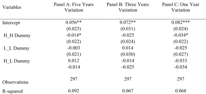
Table 9- OLS Regressions for Altman Z-score above the median of sample

Table 15 represents the regression outputs considering only companies within the sample that have Altman Z-score higher than the median of the sample. Panel A considers performance for a range of five years. Panel B represents coefficients for a range of three years. Panel C only reflects performance one year before and after the merger. H_H Dummy, L_L Dummy and H_L Dummy represent the explanatory variables. The sample comprises 594 transactions between 1990 and 2013. Robust standard errors are represented in parentheses. ***, **, * denote statistical significance at 1%, 5% and 10%, respectively.

By analyzing the results on table 9, for five years and one-year performance assessment H_H dummy variable coefficient is statistically significant at 10% significance level. Therefore, it can be seen that, on average, when a highly leveraged company acquires a highly leveraged firm, is related to a negative impact on the merged firm’s performance. Once again, these results prove the relationship between leverage and risk, creating a negative impact on performance. In table 9, the OLS coefficients are represented. The OLS estimators for control variables are represented in Appendix 7.

Variables Panel A: Five Years _Variation Panel B: Three Years _Variation Panel C: One Year _Variation

Intercept 0.056** 0.072** 0.082*** (0.023) (0.031) (0.024) H_H Dummy -0.014* -0.025 -0.034* (0.022) (0.024) (0.022) L_L Dummy -0.003 0.014 -0.025 (0.021) (0.030) (0.027) H_L Dummy 0.012 -0.014 -0.033 -0.014 -0.025 -0.034 Observations 297 297 297 R-squared 0.092 0.067 0.068

(38)

30

Table 10 - OLS Regressions for Altman Z-score below the median of sample

Table 16 represents the regression outputs considering only companies within the sample that have Altman Z-score lower than the median of the sample. Panel A considers performance for a range of five years. Panel B represents coefficients for a range of three years. Panel C only reflects performance one year before and after the merger. H_H Dummy, L_L Dummy and H_L Dummy represent the explanatory variables. The sample comprises 594 transactions between 1990 and 2013. Robust standard errors are represented in parentheses. ***, **, * denote statistical significance at 1%, 5% and 10%, respectively.

The OLS estimators presented in Table 10 (Panel B), support previous results that studies on the relationship between leverage and risk and their impact on post-merger performance (Miller and Bromiley, 1990). It appears clear that, on average, when highly levered firms with relatively lower Altman Z-Score pursue acquisition opportunities, this pursuit is associated with a negative impact on performance. When relying on a range of five years to assess the performance of a merger, the time period appears to be too extensive for our analysis to properly distil the impact of leverage.

Panel C: One Year Variation Intercept 0.098** 0.157*** 0.086* (0.047) (0.058) (0.045) H_H Dummy -0.026 -0.056* -0.018 (0.030) (0.032) (0.027) L_L Dummy -0.018 -0.018 -0.021 (0.028) (0.028) (0.027) H_L Dummy -0.028 -0.062** -0.062** (0.031) (0.031) (0.027) Observations 297 297 297 R-squared 0.092 0.081 0.074

(39)

31

6. Conclusion and Future Research

Our innovative model studied the impact of leverage on a firm’s post-merger performance. Following the performance measure suggested by Healy et al. (1992), the five years before and after the merger were analysed. For a sample of 594 mergers between 1990 and 2013, we found that a highly leveraged firm acquiring either a highly leveraged company or a lowly leveraged firm had a negative and significant impact on the post-merger performance of the majority of our cases. This effect is verified when the timeframe is changed to the three and one pre- and post-merger years. When broadening our analysis to the five-year timeframe however, the statistical significance disappears. We posit that this likely occurs due to the dilution of the leverage effect when analysing performance over a more extended timeframe.

When the same methodology was applied to years when there was an economic expansion at the macroeconomic level, we found that a highly leveraged firm acquiring a lowly leveraged firm was associated with a negative impact on post-merger performance. For recession years, we found no such relationship between leverage and post-merger performance.

Finally, we applied our model to different risk categories. For this purpose, we divided our sample into two parts: the first considered transaction acquirers with Altman Z-scores above the median, while the second considered transaction acquirers that had Altman Z-scores below the median. In cases where the Altman Z-Score was lower than the median of the sample, we found that on average, when highly leveraged companies acquire another highly leveraged firm, was correlated to a negative impact on performance. The former occurs for three-year performance analysis. Finally, when a one-year margin was analysed, we found that highly leveraged firms acquiring lowly leveraged companies typically led to a deterioration in performance. Similar results were found to Altman Z-Score higher than the median of the sample, in which highly leveraged companies acquiring a highly leveraged firm, was associated with a negative impact on performance.

Overall, our results show that when acquiring firms are highly levered, this will typically lead to a negative impact on post-merger performance. The limiting of our study to the five years before and after the merger prevents us from providing any additional results or analyses on possible longer-term effects on firm’s post-merge performances. Increasing the timeframe for analysis within our study would, unfortunately, simultaneously and significantly reduce our sample size, thereby diminishing the quality of our analysis. Thus, retrieving further data for

(40)

32 all companies involved in M&A in order to obtain a higher amount of observations and expand our horizon understudy would be a valuable avenue for additional and future research.

Furthermore, the importance of our study is very much interconnected with LBOs. Private equity firms rely on this financing scheme for the purposes of acquiring private firms. In our work here, we studied only the impact of leverage on public firms from the US. One could potentially apply our model on acquisitions to the private equity sector.