EDP Renewables
Equity Valuation Thesis
David Amaral Salgueiro
Supervisor: Professor José Carlos Tudela Martins
Dissertation submitted in partial fulfillment of requirements for the degree of MSc in Finance, at Católica Lisbon School of Business & Economics, 10 December 2016
This dissertation valuates EDP Renewables, a subsidiary company from EDP, listed on PSI20, operating in the Utilities industry - renewables energies field. Due to the energy sector transformations, the continuous search for clean sources of power plus the plausible worldwide utilities industry transformation, becomes imperative to valuate companies that can be game changers. To achieve the value per share it was used the Discounted Cash Flow, both the Free Cash Flow to the Firm & the Free Cash Flow to Equity approaches, giving us an equity value of m7.569€ and m7.564€ respectively – this translates in an 8.68€ and 8.67€ price per share. Based on the Dividend Discount Model, the equity value is m7.555€ meaning a price per share of 8.66€. According with the Multiples EV/Revenue, EV/EBITDA and Price/CF per share, we reached prices of 8.19€, 8.88€ and 8.57€. A real option approach was also developed to quantify a recent investment project (wind farm) in the UK. Due to the uncertainty related with the industry and the markets, sensitivity analysis were incorporated into the model to absorb real life volatility. In the end, we reached a final price of 8.6€ per share and we recommend a buy action (actual price: 7.11€). As benchmark for the final price per share were used valuations from Morgan Staley (8.3€) and Haitong Bank (8.2€) which allowed us to conclude that the value reached in this thesis is in line with the opinion of others financial institutions and provides this dissertation with practical usefulness.
Resumo
Esta dissertação tem como missão avaliar financeiramente a empresa EDP Renováveis, subsidiária da EDP, S.A, listada no PSI20 que opera no mercado das energias renováveis. Devido às transformações do sector, à procura contínua de fontes de energia limpa e a uma plausível transformação do modelo de negócio das Utilities a nível mundial torna-se pertinente avaliar empresas que podem desempenhar um papel crucial nesta mudança. Para obter o valor por acção recorreu-se ao método de Discounted Cash Flow method, foram usados ambos o Free Cash Flow to the Firm e o Free Cash Flow to Equity que indicou um valor de m7.569€ e m7.564€ para o capital próprio o que se traduz num preço por acção de 8.68€ e 8.67€. Com base no modelo Dividend Discount Model o capital próprio é de m7.555€ e um preço por acção de 8.66€. Através dos múltiplos EV/Revenue, EV/EBITDA e Price/CF per share, os preços alcançados foram de 8.19€, 8.88€ e 8.57€ por acção. Foi ainda desenvolvido uma avaliação de um recente projeto de investimento (parque eólico) no UK com base em real options. Devido à incerteza inerente da indústria e dos próprios mercados financeiros foram também criados senários de sensibilidade para incorporar a volatilidade do mundo real. Em termos comparativos, foram revistas avaliações financeiras do Morgan Stanley (8.3€) e do Haitong Bank (8.2€) o que nos permite concluir que os valores alcançados nesta tese estão em harmonia com a opinião de bancos internacionais de investimento e caracteriza esta tese com utilidade prática.
The cumulative knowledge that I have been incorporating since the beginning of my bachelor degree and now during the master program is expressed in this thesis dissertation.
After a three-year program and an internship of one year I was convinced to pursuit a master program in finance. Now, that my University path is coming to an end I truly believe that my choice was the right one. I strongly believe that all the knowledge about the several financial fields that I absorbed in the master program will provide a milestone in my career along with invaluable experiences that will allow me to become a successful, innovative professional and assist in accomplishing my goals. By working under the guidance of your distinguished organization, I was certainly able to exploit my potential to the fullest.
Despite the individual process of learning, without the help and collaboration of others, this path of mine would not be possible. I express here my gratitude to the Professor José Carlos Tudela Martins for his seminars and very valuable advices and help during this dissertation; to the Investor Relations Department of the EDP Renewables; to all the University community that have contributed for my growth as a person and professional and last but not the least to my family, in particular to my patents, my sister and my uncle that have created all the conditions for me to accomplish this goal of mine.
1. Introduction ... 1
2. Literature Review ... 3
2.1. Introduction ... 3
2.2. Discounted Cash Flow Methods (DCF) ... 4
2.2.1. Terminal Value ... 6
2.2.2. Adjusted Present Value (APV) ... 6
2.3. Dividend Discount Model (DDM) ... 8
2.4. Returns Based Approach ... 9
2.4.1. Economic Value Added (EVA) ... 9
2.4.2. Dynamic ROE ... 10
2.5. Relative Valuation ... 10
2.5.1. Peer Group ... 11
2.5.2. Multiples ... 12
2.6. Option Pricing Theory ... 12
2.7. The Cost of Capital ... 14
2.7.1. Weighted Average Cost of Capital (WACC) ... 14
2.7.2. Cost of Equity ... 14
2.7.3. Cost of Debt ... 15
2.7.4. Capital Asset Pricing Model (CAPM) ... 15
2.8. Further Considerations ... 17
2.8.1. Cross-border Valuation ... 17
2.8.2. Utilities Valuation ... 17
3. World Economic Outlook ... 19
4. Industry Overview ... 21
4.1. Industry Changing ... 21
4.2. Major Players ... 21
4.3. Renewables Energy Advantages ... 22
4.4. Economic Viability ... 23
4.5. Governmental Political Support ... 24
4.6. European Reform of the Emissions Licenses ... 25
4.7. The future of Energy ... 25
5. Company Overview ... 28
5.1. Introduction ... 28
5.2. Share Performance and Shareholder structure ... 29
5.3. Portfolio ... 30
5.4. Operational Performance ... 31
5.5. Financial Performance ... 32
5.5. Operational and Financials by Region ... 33
6. Valuation ... 35 6.1. Introduction ... 35 6.2. Macro Assumptions ... 35 6.3. Market Assumptions ... 37 6.3. Micro Assumptions ... 38 6.4. Company Assumptions ... 40 6.5. Historical Data ... 41
6.6. Business Plan 2016-2025 Forecast ... 45
6.7. CAPM ... 54
6.8. Market Cost of Debt ... 55
6.9. WACC ... 56 6.10. DCF ... 57 6.10.1. FCFF... 57 6.10.2. FCFE ... 58 6.11. DDM ... 59 6.12. Multiples ... 59 6.12.1. EV/Revenue ... 60 6.12.2. EV/EBITDA ... 61
6.12.3. Price/CF per share ... 62
6.12.4. Resume and Different Scenarios ... 63
6.13. Option Valuation ... 64
6.14. Sensitivity Analysis ... 65
6.14.1. Single variables ... 65
6.14.2. Scenarios Analysis ... 67
6.14.3. Monte Carlo Analysis ... 68
6.15. Valuation Resume ... 71
6.16. Valuation Comparison ... 73
7. Conclusion ... 75
8. Annexes ... 76
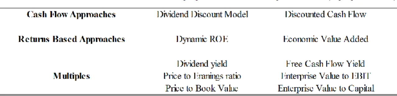
Figure 1 – Valuation Approaches ... 4
Figure 2 - FCFF vs. FCFE ... 5
Figure 3 – Economic Indicators ... 19
Figure 4 - Commodities and Utilities Indicators ... 20
Figure 5 - Renewable Energy Industrial Index by market capitalization (10/2016) ... 22
Figure 6 - Electricity Forecasts ... 27
Figure 7 - EDPR main 2015 Indicators ... 28
Figure 8 - EDPR Share Price evolution and other Indexes ... 29
Figure 9 - EDPR Share price details ... 29
Figure 10 - EDPR Portfolio ... 30
Figure 11 - EDPR Operational Data ... 31
Figure 12 - EDPR Financial Data ... 32
Figure 13 - Financial and Operational data for Europe ... 33
Figure 14 - Financial and Operational data for North America and Brazil ... 34
Figure 15 - GDP growth 2016-2021 ... 35
Figure 16 - Inflation 2016-2021 ... 35
Figure 17 - Tax rate 2016-2021 ... 36
Figure 18 - Exchange Rates 2016-2021 ... 36
Figure 19 - Commodity Prices 2016-2021 ... 37
Figure 20 - Net Generation 2016-2021 ... 37
Figure 21 - Electricity Demand 2016-2021 ... 37
Figure 22 - Installed Capacity 2008-2015 ... 38
Figure 23 - Load Factor and Electricity Output 2008-2015 ... 38
Figure 24 - Average Selling Price 2008-2015 ... 39
Figure 25 - Revenues and EBIT 2008-2015... 39
Figure 26- EDPR Business Plan 2016-2020 ... 40
Figure 27 - Consolidated IS 2008-1H16 ... 41
Figure 28 - Consolidated BS 2008-1H16 ... 42
Figure 29 - Capex & Cash Flow 2008-1H16 ... 44
Figure 33 - Assumptions for RoE ... 49
Figure 34 - Assumptions for North America ... 50
Figure 35 - Assumptions for Brazil ... 51
Figure 36 - IS 2015-2025 ... 52
Figure 37 - BS, Asset Base, PPE, Capex, CF, Net Debt 2015-2025 ... 53
Figure 38 - CAPM statistics ... 54
Figure 39 - Risk Premium ... 55
Figure 40 – WACC calculations ... 56
Figure 41 - FCFF results ... 57
Figure 42 - FCFE results ... 58
Figure 43 - DDM results ... 59
Figure 44 - EV/Revenue ... 60
Figure 45 - EV/EBITDA ... 61
Figure 46 - Price/CF per share ... 62
Figure 47 - Multiples, different scenarios ... 63
Figure 48 - Option valuation inputs ... 64
Figure 49 - Option valuation outputs ... 64
Figure 50 - Sensitivity Analysis, Financials... 65
Figure 51 - Sensitivity Analysis, Operational and Macro ... 66
Figure 52 - Scenario Analysis ... 67
Figure 53 - Monte Carlo Analysis, Europe ... 68
Figure 54 - Monte Carlo Analysis, North America ... 69
Figure 55 - Monte Carlo Analysis, Brazil ... 70
Figure 56 - Average Price per share per method ... 71
MW Megawatt GW Gigawatt TW Terawatt MWh Megawatt hour GWh Gigawatt hour TWh Terawatt hour
EBITDA/MW EBITDA per Megawatt
RENIXX Renewable Energy Industrial Index IREA International Renewable Energy Agency
OECD Organization for Economic Co-operation and Development RoE Rest of Europe
1
1. Introduction
Every rational investor persecutes an increase in the value of his/her investment. To determine if the investment has positive value and to know the right price per share it is mandatory an objective, rigorous and well-designed valuation; choosing the right assumptions, forecasting with accuracy and treating the financial data with objectivity is crucial. Furthermore, the type of company, industry, the volatility of the markets and the heterogeneous opinions among the literature related with the different models to valuate, characterize a valuation process as not only as quantitative but also qualitative due to the different interpretations of the present and opposite beliefs about the future.
To conduct a proper valuation of EDP Renewables and in order to choose the best approach, several articles among the literature were reviewed in the next stage of this dissertation with the purpose of determining the best models available to valuate this company and approach this Industry. Since there is no consensus among the authors, a solid theoretical support is necessary to produce reliable results and not an ambiguous outcome. The third and fourth chapters of this dissertation provides a macroeconomic and Industry contextualization. This is useful for the reader who can better understand the macro and micro environment that the company faces and constitutes the very basics assumptions and general ideas for the valuation process.
In the valuation section, the economic and financial data were submitted into the models to achieve a global value for the company and hence a final stock price; the models used were the DCF (FCFF & FCFE), DDM, Multiples and Real Options valuation. Gathering these models had the purpose of assign with robustness and quality the valuation itself. Combining the major approaches ensures us a more reliable final price per share and a better understanding of the company and Industry specifics. This section includes the methodology used, the results achieved and a detailed explanation about the assumptions made.
2
The next step, after the valuation exercise, it was to conduct a sensitivity analysis to submit the models to reality changes and, in an exercise of risk management, observe the deviations in the price and in the global value when the micro and macro environment varies. Volatility in the company, industry and markets was replicated here for the major assumptions.
This dissertation ends with a comparison between the values achieved here and the ones computed by two international financial institutions - Morgan Stanley & Haitong Bank - to ensure veracity and practical relevance to the work developed within this thesis.
3
2. Literature Review
2.1. Introduction
In order to achieve an accurate value per share it’s necessary to understand all the vantages and disadvantages of the models and choose the best one that better applies depending of the company and industry context. This section analyses the existing literature, compares the pros and cons of the different approaches and selects the best valuation models to apply in this dissertation. Ultimately, the quality of a valuation depends how well the analyst understands the firm and its competitive position, its operating strategy and how well forecasts the future Parrino (2005). Goedhart, Koller & Wessels (2005) reinforce the importance of accurate forecasts.
According to Luehrman (1997) a valuation exercise relies on three crucial factors: cash, timing and risk. Despite this, different micro and macro environments lead the analysts to adopt different methodologies. For a valuation exercise the analyst shall not consider a wide range of models since that it will undermine the final result Young et al. (1999); the same authors also indicate that for a proper valuation the data and the assumptions must be consistent, existence of comparability between models, only one fair value estimation and free will for the analysts to decide about the best method.
Damodaran (2002) states that the final value is not merely quantitative. Although a strong analytical basis is crucial, the heterogeneous characteristics among companies and industries must be exploited to reach a more accurate final value. The author also indicates the timeless property of a valuation due to changes in the economy, markets and company. The likelihood of change among the assumptions across time is very high.
*
“In a market economy, a company’s ability to create value for its shareholders and the amount of value it creates are the chief measures by which it is judged.”
4
Figure 1 – Valuation Approaches
2.2. Discounted Cash Flow Methods (DCF)
This method has a great acceptance among the literature and is one of the most accepted approaches in equity valuation (Havnaer, 2012). Copeland et al. (2000) emphasizes the fact that cash is king to promote the acceptance of this method. Estridge J. & Lougee B. (2007) state that this is a crucial method to valuate a company and point out the lower susceptibility of manipulation of the Cash Flows, the same does not happen with accounting standards. As mentioned before, Luerhman (1997) qualifies a valuation as a function of cash, timing and risk; the discounted CF’s, the growth rate and the discount rate measure of the DCF method respectively.
This approach requires an estimation of the present and future earnings plus cash flows, an estimation of the CF’s, the risk for the stable growth and a discount rate. Within this method there is two perspectives: The Free Cash Flow to the Firm (FCFF) and the Free Cash Flow to Equity (FCFE). The first one is the expected CF from operations, after taxes and before interest payment plus company investments. It also reflects all the CF’s available for all the financial parties.
𝐹𝑖𝑟𝑚 𝑉𝑎𝑙𝑢𝑒 = ∑ 𝐹𝐶𝐹𝐹𝑡 (1 + 𝑊𝐴𝐶𝐶)𝑡 𝑁
𝑡=1
5
Table 2 - Differences between FCFF vs. FCFE
FCFF FCFE
Cash Flows Pre Debet CF Post Debt CF
Expecyed Growth Growth in Operating Income Growth in Net Income
Discount Rate WACC Cost of Equity
Source: McKinsey Figure 2 - FCFF vs. FCFE
The second one is the CF available to pay dividends, which is also the FCFF net of all payments to debt holders.
𝐸𝑞𝑢𝑖𝑡𝑦 𝑉𝑎𝑙𝑢𝑒 = ∑ 𝐹𝐶𝐹𝐸𝑡 (1 + 𝑟𝑒)𝑡 𝑁 𝑡=1 Hence: 𝐹𝐶𝐹𝐸 = 𝐹𝐶𝐹𝐹 − 𝐼𝑛𝑡𝑒𝑟𝑒𝑠𝑡 × (1 − 𝑡) + ∆ 𝑁𝑒𝑡 𝐷𝑒𝑏𝑡
Theoretically, due to the direct relations between the two methods, considering coherent assumptions, the final value should be the same. However, considering the differences in the table below, in practice, the methods differ.
According to Pinto et al. (2010) if the company is levered, has a negative FCFE or a changing capital structure the choice must go to the FCFF method due to the fact that the cost of equity (𝑟𝑒) is more sensible to changes in the capital structure.
The Discounted Cash Flow Method has some limitations. Luerhman (1997) argues that companies with complex capital structures, strategies of fund raising and tax positions may lead to an increase in the number of errors in the valuation. Another issue is related with the estimation of the Weighted Average Cost of Capital (WACC), this one is sensible to tax shields, issue costs, debt securities and volatile capital structures (Luerhman 1997).
Fernández (2003) also points out the problem of some analysts using book values to compute the weights in the WACC, only market values shall be used within this method. According with Damodaran (2002) the analysts don’t have access to all information available to build some assumptions and due to this the intrinsic value is never the real one.
(2)
6
The DCF method, in both senses, will be used to perform the valuation exercise due to its positive attributes and to the non-existing disadvantages of this method in the company structure.
2.2.1. Terminal Value
It is impossible to estimate all the cash flows ad infinitum. To address this problem, it’s necessary to assume a steady growth and a constant reinvestment of its operating profits – also translated in the Return on Invested Capital (ROIC). Young et al. (1999) states that this is the most important element in a valuation, the figure obtained represents 80% to 90% of the all valuation value.
According with Damodaran (2012) there are three approaches to deal with the terminal value. Firstly, the liquidation in the final year of all the assets and how much they worth in market prices after debt repayments. Secondly, apply market multiples to the company’s earnings or sales revenues from the terminal year to reach the terminal value; multiples today contain the expected future growth. Mixing a DCF valuation with a relative one may reduce the accuracy of the valuation. Thirdly, the stable growth model assumes a perpetual reinvestment of a percentage of the CF’s into new assets (by opposite with the liquidation model), a stable growth and assumes also that the company is already in a steady-state.
𝑇𝑒𝑟𝑚𝑖𝑛𝑎𝑙 𝑉𝑎𝑙𝑢𝑒𝑡 = 𝐶𝐹𝑡+1 𝑅 − 𝑔
The perpetual growth rate (𝑔) represents a limitation of this method. It is impossible for a company to growth always more than the overall growth of the world economy (Damodaran 2005).
“One practical drawback common to all present value models is that they are highly sensitive to things we do not know. More specifically, the terminal value is usually by far the most important element in any valuation estimate and yet it is extraordinarily difficult to estimate it with any degree of accuracy.” (Young et al., 1999).
2.2.2. Adjusted Present Value (APV)
Regarding the issues discussed above about the DCF method emerges another method that nowadays has also acceptance among the literature. In the APV method the value of a
7
company is computed based only in equity financing and then posteriorly adding the present value of the expected tax benefits and subtracting the bankruptcy costs. Luehman (1997) states that this method provides transparency due to the fact that all the components are separated which allows a better view of the methodology.
𝐴𝑃𝑉 = 𝑃𝑉𝐶𝐹 𝐴𝑠𝑠𝑒𝑡𝑠 + 𝑃𝑉𝐴𝑙𝑙 𝑓𝑖𝑛𝑎𝑛𝑐𝑖𝑛𝑔 𝑠𝑖𝑑𝑒 𝑒𝑓𝑓𝑒𝑐𝑡𝑠
Once the company is valuated exclusively equity based, i.e. unlevered, it is necessary to compute the present value of the expected tax benefits (tax shields) and the bankruptcy costs. Relatively to the tax benefits, Damodaran (2006) points out the importance of choosing the right tax rate and if this rate may change across time, to know what is the right level of debt and if this level may change over time and finally what discount rate to use to reach the present value.
𝑃𝑉𝑡𝑎𝑥 𝑠ℎ𝑖𝑒𝑙𝑑𝑠 =𝐷𝑒𝑏𝑡𝑡∗ 𝐼𝑛𝑡𝑒𝑟𝑒𝑠𝑡 𝑅𝑎𝑡𝑒𝑡∗ 𝑇𝑎𝑥 𝑅𝑎𝑡𝑒𝑡 (1 + 𝑟𝑑)𝑡
Respectively to the bankruptcy costs, Damodaran (2006) argues that this is the larger issue in APV because those costs represent a large amount and their probability and exact amount are difficult to estimate with accuracy.
𝐸(𝐵𝑎𝑛𝑘𝑟𝑢𝑝𝑡𝑐𝑦 𝐶𝑜𝑠𝑡𝑠) = 𝑃𝑟𝑜𝑏𝑎𝑏𝑖𝑙𝑖𝑡𝑦 𝑜𝑓 𝐷𝑒𝑓𝑎𝑢𝑙𝑡 × 𝐵𝑎𝑛𝑘𝑟𝑢𝑝𝑡𝑐𝑦 𝐶𝑜𝑠𝑡𝑠
The cons about the second equation are the lack of consensus about how to compute both terms. Damodaran (2002) suggests an approach based on the trading bonds ratings to reach the probability of default or consult specific rating agencies. For the Costs, Branch (2002) says that the figure should be around 28% of the pre-distressed company’s value.
The final step of the APV method is to reach the levered value of the company adding up all the variables. Hence:
𝑉𝐿 = 𝑉𝑈+ 𝑃𝑉𝑡𝑎𝑥 𝑠ℎ𝑖𝑒𝑙𝑑𝑠+ 𝐸𝐵𝐶
APV method is mostly used and outperforms FCF when the capital structure of company is expected to change substantially during the investor horizon. Since the historical ratio of
(5)
(6)
(7)
8
our company is significantly stable, its politics is to keep it in that way and due to the issues of the method itself and its possible lack of accuracy this method won’t be applied.
2.3. Dividend Discount Model (DDM)
This section approaches the Dividend Discount Model (DDM) firstly present by Williams in 1938 and then updated by Gordon and Shapiro in 1956. It only considers dividends as cash flows to equity and assumes that shareholders expect to receive dividends payment during the holding period plus a price when they sell their share (Damodaran 2002). According with Foerster & Sapp (2005) the risk of CF’s from equity comes from the timing and growth associated with the company’s earnings and the availability in paying dividends. Relying on the present value of the summation of all expected future dividends, using cost of equity to discount them, the company’s stock price is obtained.
Following Damodaran (2005), depending on the growth forecasts, the model must be applied in two different ways:
𝑆𝑡𝑎𝑏𝑙𝑒 𝐺𝑟𝑜𝑤𝑡ℎ 𝑀𝑜𝑑𝑒𝑙: 𝑃0= 𝐸𝑥𝑝𝑒𝑐𝑡𝑒𝑑 𝐷𝑃𝑆 𝐾𝑒− 𝐸𝑥𝑝𝑒𝑐𝑡𝑒𝑑 𝐺𝑟𝑜𝑤𝑡ℎ 𝑖𝑛 𝑃𝑒𝑟𝑝𝑒𝑡𝑢𝑖𝑡𝑦 𝑇𝑤𝑜 𝑆𝑡𝑎𝑔𝑒𝑠 𝑔 𝑀𝑜𝑑𝑒𝑙: 𝑃0= ∑ 𝐸(𝐸𝑃𝑆𝑡) (1 + 𝐾𝑒𝑡) 𝑛 𝑡=1 + 𝐸(𝐷𝑃𝑆𝑛+1) 𝐾𝑒− 𝐸𝑥𝑝𝑒𝑐𝑡𝑒𝑑 𝐺𝑟𝑜𝑤𝑡ℎ 𝑖𝑛 𝑃𝑒𝑟𝑝𝑒𝑡𝑢𝑖𝑡𝑦 (1 + 𝐾𝑒)𝑡
Only the expected dividends, obtained through out future growth assumptions and the cost of equity, are necessary to apply the equations. Damodaran (2006) highlights the simplicity and intuitive understanding of the model and its accurate estimations of the value per share when companies pay out their free cash flows to equity in the form of dividends.
Despite the apparent facility and effectiveness of the method, this model has some drawbacks. Paying dividends is a political decision: some companies do not pay them, others only do it in punctual years and some even increase debt to be able to do it and to give a (fake) signal to the market. Moreover, expecting a constant dividend growth is not suitable for the all the companies. If the company holds back cash this leads to an undervalued price per share, if it uses debt or equity to pay dividends this leads to an
(10) (9)
9
overvalued price per share. This methodology can only be applied in specific cases, in companies with specific characteristics otherwise leads the analyst to inaccurate valuations. Due to the regular and consistent dividend’s payments of our company, this model will be also used.
2.4. Returns Based Approach
The models discussed so far do not indicate directly to investors the company’s performance. The following to models are designed based on profitability and aim to address in which terms the company produces value or not.
2.4.1. Economic Value Added (EVA)
This method intends to account the excess value produced by an investment comparing the company’s cost of capital and its return on the invested capital. Damodaran (2005) classifies EVA as an indicator of the increase in value created by an investment or a portfolio of investments. Shareholders’ interests tend to be more addressed with this method due to the computation of the value created with the new investment that, if positive, represents a good indicator of a future payback.
𝐸𝑉𝐴 = 𝐴𝑓𝑡𝑒𝑟 𝑇𝑎𝑥 𝑂𝑝𝑒𝑟𝑎𝑡𝑖𝑛𝑔 𝐼𝑛𝑐𝑜𝑚𝑒 − 𝐶𝑜𝑠𝑡 𝑜𝑓 𝐶𝑎𝑝𝑖𝑡𝑎𝑙 × 𝐶𝑎𝑝𝑖𝑡𝑎𝑙 𝐼𝑛𝑣𝑒𝑠𝑡𝑒𝑑
According with Damodaran (2005) the estimation of the capital invested and the cost of capital it is crucial. The first one relies on the capital invested initially plus the cumulative market value; the second is the market measure of the cost. Book values must be ignored. Salmi et al. (2001) identified higher sensitivity from EVA to the cost of equity and lower sensitivity to the cost of debt. Moreover, specific management policies as pursuing growth or leverage tend to affect substantially this methodology. Hence, using this method requires a understanding of the intern policies and the macroeconomic environment.
10
Damodaran (2005) associates Enterprise Value with the EVA model in the following equation where the value comes from the capital invested in assets plus the present value of these same assets plus the value added by the future projects.
𝐸𝑉 = 𝐼𝑛𝑣𝑒𝑠𝑡𝑒𝑑 𝐶𝑎𝑝𝑖𝑡𝑎𝑙 + ∑𝐸𝑉𝐴𝑡 𝑎𝑠𝑠𝑒𝑠𝑡 𝑖𝑛 𝑝𝑙𝑎𝑐𝑒 (1 + 𝑊𝐴𝐶𝐶)𝑡 + ∑ 𝐸𝑉𝐴𝑡 𝑓𝑢𝑡𝑢𝑟𝑒 𝑝𝑟𝑜𝑗𝑒𝑐𝑡𝑠 (1 + 𝑊𝐴𝐶𝐶)𝑡 𝑛 𝑡=1 𝑛 𝑡=1 2.4.2. Dynamic ROE
This approach is very similar to the one discussed above, the difference relies in the fact that this method has its perspective over equity instead of the enterprise. The dynamic ROE compares the return on equity (ROE) with the cost of equity (𝐾𝑒).
𝑉𝑒𝑞 = 𝐸0 × ∑ 𝐸𝑡−1× (𝑅𝑂𝐸 − 𝐾𝑒) (1 + 𝐾𝑒)𝑡 𝑛 𝑡=1 *
The two models addressed in the Returns based approach chapter differ from the previous ones in the sense that provides us information about the economic profit that has been generated by the company. However, since this methodology relies more into accounting information and the time horizon is considerably short, their acceptance is not universal and hence they will not be considered.
2.5. Relative Valuation
Within this methodology the value of an asset is derived from the pricing of others similar assets and to do so it is used a common variable like earnings, revenues, cash flows or book value; relative valuation reaches the value of an asset by looking to the market and seeing how much worth it similar assets Damodaran (2006). This method, due to its straightforward application and immediate output, allows companies to understand its
(12)
11
positions among its peers. Asquith et al. (2005) says that the majority of top analysts uses multiples for enterprise valuation.
Lie et al. (2001) point out this method as a facilitator for understanding other valuations since the results provided by multiples are easy to read. They also defend its application as a complement to other valuation methods. Fernandez (2002) also supports this methodology but also as a complement to others methods. Furthermore, Goedhart et al. (2005) states that the relative valuation and the DCF should be combined in the valuation exercise.
For Ferris & Pettit (2013), “multiple is a ratio between two financial variables. In most cases, the numerator of the multiple is either the company’s market price (in the case of price multiples) or its enterprise value (in the case of enterprise value multiples). The denominator of the multiple is an accounting metric, such as the company’s earnings, sales, or book value.”
2.5.1. Peer Group
For an accurate relative valuation, it’s necessary a well-designed peer group, the companies within the group must share similar characteristics to allow a comparison between them. According with Damodaran (2006) comparable firms do have similar cash flows, growth pattern, and same level of risk. For Koller et al. (2005) the peer group must share a similar return on invested capital (ROIC) and the same level of growth in the long-run.
Moreover, Liu et al. (2012) defend that choosing companies from the same industry increases the accuracy of the valuation. Foushee et al. (2012) states that for this analysis the companies should operate in similar markets and face the same macro-economic environment.
The main drawback about this methodology is to create a list with companies that share a large amount of similarities with the company under valuation. Damodaran (2006) also points out that the quality of the result depends of how good the market evaluates the others companies into the peer group. For instance, a general undervaluation of the group translates into an undervalued valuation for the company in analysis.
12 2.5.2. Multiples
According with Goedhart et al. (2003), to use the multiples approach, an analyst must consider some basic steps: peers with similar ROIC and growth pattern, apply forward-looking plus enterprise-value multiples and adjust enterprise-value multiples for non-operating items.
Liu et. al. (2001) and Kim and Ritter (1999) are also in favor of using forward-looking multiples due to a more accurate outcome. The most used are the Price-to-earnings ratio (PER) and the Enterprise-Value multiples (EV), this last one can have as the denominator EBITDA, Sales, EBIT and Capital for instance. According with Fernandez (2001) the major ones are the PER and the EV/EBITDA.
Nevertheless, according with the industry in analysis, the preference changes: for Utilities the author refers the PER and the Price to cash flow (P/CF). Despite this industry segregation, Lie and Lie (2002) state that the application of several multiples performs better than the application of only a few.
𝑃𝐸𝑅 =𝐶𝑢𝑟𝑟𝑒𝑛𝑡 𝑀𝑎𝑟𝑘𝑒𝑡 𝑃𝑟𝑖𝑐𝑒 𝐸𝑎𝑟𝑛𝑖𝑛𝑔𝑠 𝑝𝑒𝑟 𝑆ℎ𝑎𝑟𝑒 𝐸𝑛𝑡𝑒𝑟𝑝𝑟𝑖𝑠𝑒 𝑉𝑎𝑙𝑢𝑒 𝑀𝑢𝑙𝑡𝑖𝑝𝑙𝑒𝑠 = 𝐸𝑉 𝐸𝐵𝐼𝑇𝐷𝐴 𝑜𝑟 𝑆𝑎𝑙𝑒𝑠 𝑜𝑟 𝐸𝐵𝐼𝑇 𝑜𝑟 𝐶𝑎𝑝𝑖𝑡𝑎𝑙 𝑃𝑟𝑖𝑐𝑒 𝑡𝑜 𝐶𝑎𝑠ℎ 𝐹𝑙𝑜𝑤 = 𝑆ℎ𝑎𝑟𝑒 𝑃𝑟𝑖𝑐𝑒 𝐶𝑎𝑠ℎ 𝐹𝑙𝑜𝑤 𝑝𝑒𝑟 𝑆ℎ𝑎𝑟𝑒
Due to its large acceptance as a support valuation model and its immediate and comparable results this approach will be considered in the valuation exercise.
2.6. Option Pricing Theory
This methodology reaches the value based on options, derivative securities that derive its value based on an underlying asset. According with Damodaran (2002) this method can be useful to value assets whose value varies depending on the intrinsic characteristics of options whose value cannot be reached conventionally. Moreover, when the company has substantial operations’ volatility, this method can be applied.
(15)
(16) (14)
13 Binomial Model
Black Scholes Model
S - current value of the underlying asset K - strike price of the option
t - option expiration life r - risk free interest rate
- variance of the underlying asset 𝑆𝑢 𝑆 𝑆𝑑 𝑆 𝑆𝑢 𝑆
S is the current stock price and moves up to Su with probability p and moves down to Sd with probability 1- p.
More recent literature states that due to the necessity of management to adjust its decisions to address unexpected events, due to the fact that companies do learn and respond to new developments the DCF model may not capture it. Hence, the option price theory can be used allowing managers to adjust decisions to the new faced environment (Trigeorgis 1993).
Luerhman (1997) states that this method should be a complement to other methodologies and not being used as a single valuation model. Furthermore, Wooley and Cannizzo (2005) argue that DCF undervalues investment projects; Copeland and Keenan (1998) go further by saying that NPV is responsible for several underinvestment decisions across time.
The two separate models to valuate companies within this methodology are the Black Scholes model and the Binomial Model. Luerhman (1997) defends the use of the first one since it shares with DCF more inputs and thus allows a more homogeneous comparison.
The company in analysis has a premature project related with natural resources and to account its asset value this method will be applied specifically to this investment project.
(18) (17)
14
X/(E+D+P) - market value proportion of X in funding mix Ke - cost of equity
Kd - cost of debt
Kp - cost of preferred stock T - tax rate
Ke - cost of equity Rf - risk-free rate
(Rm - Rf) - market risk premium β - beta
2.7. The Cost of Capital
To reach the present value of the future cash flows it’s required a discount rate which reflects the cost of money, it represents the opportunity cost of investing in a particular project instead of allocate the capital to another one. Cost of equity for projects only financed with equity, cost of debt when using debt only and the weighted average cost of capital for a mixed solution.
2.7.1. Weighted Average Cost of Capital (WACC)
“The required return for the equity holders and debt holders taking into account the proportion in which way the company is financed and embedded in this rate are the tax benefits of the debt.” Miles & Ezzell, 1980
𝑊𝐴𝐶𝐶 = 𝐸 𝐸 + 𝐷 + 𝑃× 𝐾𝑒+ 𝐷 𝐸 + 𝐷 + 𝑃× 𝐾𝑑 × (1 − 𝑇) + 𝑃 𝐸 + 𝐷 + 𝑃× 𝐾𝑝
Although the simplicity of this method, the literature only approves this methodology for companies with a relatively stable capital structure. Luerhman (1997) states the lack of efficiency of WACC for companies with complex tax structures.
2.7.2. Cost of Equity
This represents the expected return for an investor who invests in a project and faces the risk of it. Following Damodaran (2001) and Koller et al. (2005), to reach the cost of equity the most used approach is the Capital Asset Pricing Model (CAPM) – further discussed in more depth.
𝐾𝑒 = 𝑅𝑓+ 𝛽𝐿[𝐸(𝑅𝑚− 𝑅𝑓)]
(19)
15 2.7.3. Cost of Debt
According with Damodaran (2006) the cost of debt incorporates the default risk and the market interest rates. Thus, it reflects the cost of borrowing money for a company. Due to the fact that interest payments are tax deductible is often computed the after tax cost of debt i.e. the effective rate. The cost has the risk free component plus the premium demanded by investors to invest in a specific company (Damodaran 2002).
𝐾𝑑 = 𝑅𝑓+ 𝑃𝑟𝑒𝑚𝑖𝑢𝑚
The premium component can be obtained based on the company’s yield to maturity (YTM) of long term bonds, based on the estimation of the default spread on the company’s credit rating or based on the recent borrowing company’s rates.
2.7.4. Capital Asset Pricing Model (CAPM)
As briefly discussed before in the cost of equity section of this dissertation the CAPM1 is widely used to estimate companies’ cost of capital and evaluate the performance of investment portfolios.
Fama and French (2004) state that this methodology “offers powerful and intuitively pleasing predictions about how to measure risk and the relation between expected return and risk”. According with the model the investor must be remunerated for the risk taken and for the time value of the money invested, this last one is measured by the risk-free rate in the following equation:
𝐾𝑒 = 𝑅𝑓+ 𝛽[𝐸(𝑅𝑚− 𝑅𝑓)]
2.7.4.1. Risk Free
According Damodaran (2005) the risk free rate must have no default risk and no reinvestment risk. Only government bonds, not all by far, apply for this criteria based on the principle that they can print their currency. The maturity of the bonds must match investment horizon.
1 Introduced by Sharpe in 1964; further developed by Markowitz, Fama & French (1992) and Carhart (1997).
(21)
16
The risk free rate is the return of a portfolio which has no covariance with the market, those rates in the long-term government bonds in the US and Western Europe do have a significantly low covariance relationship with the market (Koller et all., 2005).
2.7.4.2. Beta
The β variable in the equation measures the volatility or the systematic risk of the company relative to its market adjusted for the level of leverage. Due to the fact that debt is tax deductible and provides tax benefits, the levered beta contains a lower level of volatility than the unlevered one.
Following Damodaran (2002), this presents two ways of computing beta: raw beta (levered) and adjusted beta. The raw beta is reached through a regression of the stock markets versus the market returns and gives us an historical measure. The adjusted one is merely an estimation for the future beta of the company.
𝑅𝑎𝑤 𝛽: 𝑅𝑎 = 𝛼 + 𝛽𝑅𝑚 𝑤𝑖𝑡ℎ: 𝛽 =(𝐶𝑜𝑣(𝑅𝜎𝑎,𝑅𝑚)) 𝑚2 𝐴𝑑𝑗𝑢𝑠𝑡𝑒𝑑 𝛽 =2 3 × 𝑅𝑎𝑤 𝛽 + 1 3 To reach the unlevered beta it is used the following equation:
𝛽𝐿 = 𝛽𝑈 × [1 + (1 − 𝑡) ×
𝐷 𝐸]
2.7.4.3. Risk Premium
The trade-off risk-return states that the higher the level of risk in an investment the higher must be the return to compensate the investor for facing riskier conditions. As reasons to justify facing the risk we have the diversifiable risk (company related) and the non-diversifiable risk (market related). The first one affects a specific investment or position while the second one impacts a higher amount of investments.
The risk premium consists in the difference between the expected return on an investment and the risk free rate gathering all of these three concepts: historical market risk premium, required market risk premium, expected market risk premium.
(23)
17 T - number of observations
N - period to forecast in years Ra - arithmetic average Rg - geometric average
According with Damodaran (2011), to estimate the risk premium, one has several distinct methods. For instance: the historical premium approach which consists in computing the premium based on the average historical differences between the market returns and the risk free rates across a long period; the implied equity premium approach focusing on the estimation of forward-looking premiums based on the prices of today’s market.
This dissertation uses the historical approach computing the average and geometric average and then uses the Marshall Blume estimator to adjust estimations errors and autocorrelations returns. 𝑅𝑝 =𝑇 − 𝑁 𝑇 − 1× 𝑅𝑎 + 𝑁 − 1 𝑇 − 1× 𝑅𝑔 2.8. Further Considerations 2.8.1. Cross-border Valuation
Evaluate a company that operates overseas rises the necessity of addressing issues related with international operations. Kester and Froot (1997) and Koller et al. (2010) refer the foreign currencies associated with the cash flows and with the cost of capital as the major ones. Despite the currency used, the intrinsic value must be the same (Koller et al. 2010). According with the same author there are two methods to address this situation: (1) run the model and then, in the end, use spot exchange rates to convert all the figures into the same currency; (2) use forward exchange rates to convert the forecasted cash flows for the following years and then, once discounted, they will all be already in the same currency.
2.8.2. Utilities Valuation
Each Industry may require different approaches and some adjustments to the valuation methods. The methodology to valuate a bank or an industrial company strongly differs due to their differences in the financial accounts.
18
Multiples seem to be the approach with more adjustments requires depending of the industry (Blacconieri et al. 2000).
The Utilities industry is strongly legislated and cross-agreements between the companies, private and governmental agencies within the industry and the government itself are common. Menegaki (2008) recommends adjustments for this industry, model based valuations about environmental, resource and energy economics.
19
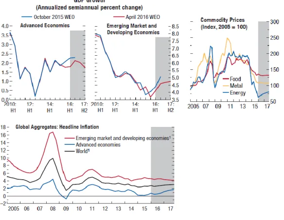
Figure 3 – Economic Indicators
3. World Economic Outlook
This chapter aims to provide the reader with macroeconomic and financial illustrative data about the past, current and forecasted worldwide economic and financial situation. It has general economic indicators and some more specific measures for the commodities and utilities sector. The ultimate purpose is to present economic and financial information about the macro environment and to serve as the very basis for the valuation assumptions.
3.1. Economic and Financial Indicators
According with the World Bank the worldwide GDP will have a non-growth for advanced economics and it will increase for emerging markets, inflation will remain flat and the price of energy will rise after a significant drop.
20
Figure 4 - Commodities and Utilities Indicators
3.2. Commodities and Utilities related
Important observations such as the decrease in the use of coal for electricity generation, substantial increase in the share of electricity production via clean energies and a sharp decrease in the costs of R&D for renewables sources of energy are positive indicators and anticipate a bright future for renewable energy companies.
21
4. Industry Overview
4.1. Industry Changing
Nowadays, the discussion over the world’s future energy is ongoing and concerns a huge number of institutions: governments, private industrial companies from several industries, financial sector and others. The world demand for energy for the next 20 years it will growth over 30% and the necessity to address this issue and at the same time prevent climate change and greenhouse gases opens a path even more optimistically for renewable energies.2
The energy Industry is responsible for 72% of all the emission of greenhouse gases and to control global warning this value needs to be reduced3. In December 2005, in Paris, was signed an agreement by 195 countries where they compromised to keep global warming under 2ºC. Within this scenario is imperative to give to the renewables energies a crucial role, they have proved to be a competitive energy source and to contribute for the country’s GDP.
4.2. Major Players
The top thirty major players in terms of market capitalization are identified in the Renewable Energy Industrial Index (RENIXX 30). One can observe a clear domination by the US and China (CN) with 8 companies each, followed by countries like Canada, Germany, Denmark and Spain with 2 each.
2 Intergovernmental Panel on Climate Change 2015 3 World Resource Institute 2015
22
Company Country Price per Share (€)
Albioma SA FR 15,37
Brookfield Renewable LP BM 26,92
Canadian Solar Inc CA 13,18
China High Speed Group Co CN 0,94
China Longyuan Power CN 0,72
Dong Energy DK 36,68
EDP Renovaveis SA ES 6,55
First Solar Inc US 35,42
Gamesa Corporacion Tech ES 21,26
GCL Corp. Energy CN 0,12
Innergex Renewable Energy CA 9,54
JA Solar Holdings Co Ltd CN 6,13
JinkoSolar Holding Co Ltd CN 14,87
Meyer Burger Technology CH 3,17
Nordex SE DE 26,81
Ormat Technologies Inc US 41,81
Plug Power Inc US 1,53
REC Silicon ASA NO 0,11
SMA Solar Technology AG DE 28,82
SolarCity Corp US 17,86
Solaredge Technologies Inc US 15,27
SunPower Corp US 7,84
Sunrun Inc US 5,58
SunZlon IN 0,75
Tesla Motors Inc US 175,98
Trina Solar Ltd CN 9,11
Verbund AG AT 14,95
Vestas Wind Systems DK 75,27
Xinjiang Goldwind Science & Technology Co Ltd CN 1,36
Yingli Green Energy Holding Co Ltd CN 3,41
The 30 RENIXX-World Stocks (Renewable Energy Industrial Index by market capitalization)
Figure 5 - Renewable Energy Industrial Index by market capitalization (10/2016)
4.3. Renewables Energy Advantages
According with the International Renewable Energy Agency (IREA), doubling the productivity capacity until 2030 of the renewables energies would be enough to achieve the Paris’s goals. It is expected a 34% rate of global production of clean energy by 2040.
23
Although environmental causes and issues shall be addressed usually they are bellow in terms of priorities comparatively with the economics interests. Despite possible drawbacks relatively to the progress of renewables energies this is not the case. In the present world, green energies have the power of mitigate climate changes and are classified as investments that catalyze direct and indirect economic benefits through the reduction of dependency to import energy (most often oil and gas), improving air condition and, as consequence of the economic development, improve unemployment rates.
GDP growth: the development of a new industry and new technology that represent each time more the worldwide economy.
Employment improvement: due to its labor-intensive proprieties, by opposite with fossil fuel industries more mechanical and capital-intensive, they create new jobs. According to IREA, the renewable sector employed, in 2015, 8.1 millions of people. Wind energy is responsible for more than 1 million jobs, 31% are in Europe.
Less energy dependency from other countries: since wind, solar and hydro energy are endogenous to the countries they increase its intern energy support and mitigate the exposition risk to energy import.
4.4. Economic Viability
The technological improvement pushes prices down and has been making green energy an investment with a lower initial investment. The aero-generators have seen they price decrease in one third from the past 6 years which leads to an increase in competitively; Bloomberg estimates that this source would produce 2.000 GW in 2040 (433 GW was the production in 2015). Photovoltaic panels’ prices decreased about 75% since 2009 and it is expected from them to keep this tendency. Bloomberg predict that this source of energy will rule all the new constructions in the future; 5000GW of capacity in 2040 (178GW in 2015).
It is notorious the impact of tech evolution in the Industry and how it enables the investment in renewables energy.
24 4.5. Governmental Political Support
The economic reasons, the environmental concerns and the new green policies have been boosting the growth of renewables energies all across the world.
China broke a record and completely oversteps the analysts’ forecasts creating in the past year a new power capability of 31GW. In Europe the figure was 13GW (Germany 6GW, Poland 1.3GW, France 1.1GW, UK 1GW, others 3.6GW). About North America, USA installed 8GW and Canada 2GW. Latin America created 3GW and emergent economies around also 3GW.4
The European council in the past year formulated a binding agreement between countries to achieve in 2030 a level of 27% of clean energy for the European Union (EU), a reduction of 40% in the greenhouse gases and a 27% level of energy efficiency. A report from the Environmental European Agency states that the EU it is in a good path to achieve the targets.
The following list presents the legal procedures and the government’s measures of some European countries to reach the goals of the agreement (plus the situation of the EUA):
Spain: January 2016, Spanish government opened an auction for private companies to build 700MW of renewable energy.
France: July 2015, new law pretends to cut by 40% greenhouse gases emission until 2040 and increase clean energy production up to 32% of all electricity produced.
Poland: February 2015, creation of a new system of support to all the new renewable energy companies.
Italy: 2016 1st trimester, new law bill authorizing new auctions to install up to 800MW of clean energy.
4 World Resource Institute 2016
25
UK: February 2016, British government stablishes contracts with the private sector to construct 27 projects and install more 2,1GW of renewable energy.
Romania: December 2015, for 2016 13% of all electricity produced must come from clean sources.
EUA: December 2015, more fiscal incentives (fiscal credits during 10 years) for the wind generations parks.
4.6. European Reform of the Emissions Licenses
The emissions licenses commerce was founded in 2005 with the purpose of reducing greenhouse gases emissions in a more effective and economically viable way. The agreement has pre-stablished maximum levels of emissions and this limit is reduced every year to reach the final purpose of the contract. Private companies receive and can also buy rights according with their needs. Due to the scarcity of rights and to the economic crisis the contract’s boundaries have been crossed.
To address it the European Commission created two mechanisms, in 2014 a deferral for new licenses and in 2015 a market stability reserve. The first one aims the short-term and intends to rebalance the supply and demand as decrease price volatility. The second one, focused in the long-run, pretends to decrease the historic surplus in licenses attribution and adjust better the rights given. The European Commission pretends to cut the number of licenses assigned by 2.2% per year.
4.7. The future of Energy
“Hydroelectric generation, onshore and offshore wind power, and solar photovoltaic will spearhead this transformation, which should be accompanied by improvements in networks and back-up and storage technologies.” Ignacio Galán, at the World Economic Forum 2016
According with the World Economic Forum the expected demand for energy until 2040 it will growth 40% and the necessity of comply with the Paris agreement implies new ways to
26
produce electricity, throughout renewables sources. To address both the demand and the gases restrictions a $7 billion investment is required in OECD countries.
New trends in electricity production5: Sectoral
Renewable Energy will increase in 8,300 TWh by 2040, 50% in Europe, 30% in China and Japan, 25% in the USA and India; coal will represent no more than 15% for outside Asia.
Increase in the number of policies in favor of low gases emissions energy production due to cost trends, cost of renewables continues to go down.
World population 4 times larger by 2050, unsustainability issues of natural resources.
Technological
Tech advances and better efficiency allied with political pressures to continuous development.
Smart grids will allow house automation and personal management of electricity. Technological advances for new renewables energies and for the distribution
process may change the current market model.
Electricity storage, still embryonic, will allow a personal management of the power systems.
Consumption
17% of the global population (1.2 billion people) doesn’t have access to electricity and 38% (2.7 billion) risk their health using traditional ways in order to cook. Development of new uses may create new markets and opportunities: electrical
vehicles, robots.
27
Figure 6 - Electricity Forecasts
28 Net Investment 719m € Collaborators 1018 Intalled Capacity 9,6 GW Operating CF 701m € EBITDA 1142m € EBITDA/MW 137k €/MW Production 21,4 TWh Net Debt 3,7m € Net Income 167m €
Key Figures for 2015
Figure 7 - EDPR main 2015 Indicators
5. Company Overview
5.1. IntroductionEDP Renewables integrates development, construction and operations of wind farms and solar power plants in order to produce and to sell renewable energy. Its activity is present in twelve countries (Portugal, Spain, Italy, France, Belgium, Poland, Romania, UK, Canada, USA, Mexico and Brazil) and has as geographic business regions Europe, North America and Brazil.
The amount of electricity produced worldwide in 2015 was 21.4 TWh, with an installed capacity of 9.6 GW (plus 344MW under construction), employs more than 1000 collaborators.
29 EDPR - Market 2015 2014 2013 2012 2011 Opening Price (€) 5,4 3,86 3,99 4,73 4,34 Close Price (€) 7,25 5,4 3,86 3,99 4,73 Market Cap (m€) 6324 4714 3368 3484 4124 Volume (m) 289,22 396,84 448,15 446,02 463,56 Total Return (%) 35% 41% -2% -16% 9% PSI 20 (%) 11% -27% 16% 3% -28%
Dow Jones Utilities (%) -5% 12% 9% -9% -25%
0 20 40 60 80 100 120 140 160 180 01 -0 6-20 08 01 -1 0-20 08 01 -0 2-20 09 01 -0 6-20 09 01 -1 0-20 09 01 -0 2-20 10 01 -0 6-20 10 01 -1 0-20 10 01 -0 2-20 11 01 -0 6-20 11 01 -1 0-20 11 01 -0 2-20 12 01 -0 6-20 12 01 -1 0-20 12 01 -0 2-20 13 01 -0 6-20 13 01 -1 0-20 13 01 -0 2-20 14 01 -0 6-20 14 01 -1 0-20 14 01 -0 2-20 15 01 -0 6-20 15 01 -1 0-20 15 01 -0 2-20 16 01 -0 6-20 16 01 -1 0-20 16
Indexed Chart - EDPR; PSI20; IBEX35; DJI; RENIXX
EDPR PSI 20 IBEX 35 DJI RENIXX
Figure 9 - EDPR Share price details
5.2. Share Performance and Shareholder structure
EDPR is listed in the Euronext Lisbon since 2008 – was created through an IPO. The share opened at 8€, went to 5€ in mid-2008, raised to 7.6 in later 2009 and then felt until 2.7€ in mid-2012. Since then, rose again until 7€ in later 2015 – this price has been partially constant until now.
30 Portfolio 1H2016 Installed Capacity (MW) Production (GWh) Load Factor (% ) Under Construction (MW) Market Share 2015
Canada 30 39 30% - n.a. USA 4.382 6.712 37% 429 37% Mexico - - 0% 200 0% Brazil 204 205 29% - 1% Portugal 1.249 1.751 32% 2 25% Spain 2.371 2.879 31% - 10% Italy 100 132 31% 14 1% France 376 464 29% 12 4% Belgium 71 76 25% - 3% UK - - 0% 1.116 0% Poland 418 472 24% - 9% Romania 521 583 26% - 16% -1.000 2.000 3.000 4.000 5.000 6.000 7.000 8.000 -500 1.000 1.500 2.000 2.500 3.000 3.500 4.000 4.500 5.000
Installed Capacity (MW) Production (GWh) Figure 10 - EDPR Portfolio
The shareholders are divided by 23 countries, the major one is EDP S.A. with 77.5% of all the 872.308.162 shares followed by the MSF Investment Management with 3%, the remaining 19% is distributed by other shareholders.
5.3. Portfolio
EDPR portfolio is well diversified across several countries, its larger business areas in terms installed capacity and production are the US, Spain and Portugal.
31
Operating Data 2013 2014 2015 1H16
Installed Capacity (EBITDA MW + Eq. Consolidated)8.565 9.036 9.637 9.721
Europe 4.796 4.938 5.141 5.105 North America 3.685 4.014 4.412 4.412 Brazil 84 84 84 204 Electricity Generated (GWh) 19.187 19.763 21.388 13.314 Europe 9.187 9.323 10.062 6.358 North America 9.769 10.204 11.103 6.750 Brazil 230 236 222 205 Load Factor (%) 30% 30% 29% 33% Europe 28% 27% 26% 30% North America 32% 33% 32% 37% Brazil 31% 32% 30% 29%
Average Selling Price (€/MWh) 62,6 58,9 64,0 59,9
Europe (€/MWh) 89,3 80,3 83,0 79,1 North America ($/MWh) 48,4 50,8 51,0 46,5 Brazil (R$/MWh) 309,2 346,4 370,4 265,1 Employees 890 919 1.018 1.055 Europe 467 434 445 459 North America 298 316 383 395 Brazil 23 26 32 33 Holding 102 143 158 168
Figure 11 - EDPR Operational Data
5.4. Operational Performance
EDPR possesses a diversify portfolio across Europe and America with 9.6 GW and with an average of 6 years old. The EBITDA per GW comes from Spain 46%, North America 24%, Rest of Europe 16% and Portugal 16%. By the end of 2015, to operate in 2016, EPDR had in construction 200MW in Mexico, 120MW in Brazil and 24MW in France.
In terms of Electricity production, EDPR produced in 2015 21.4 TWh – North America 52%, Spain 23%, Rest of Europe 15%, Portugal 9% and Brazil 1%.
32
Financial Data (€m) 2013 2014 2015 1H16
Revenues 1.316,4 1.276,7 1.547,1 888,9
Operating Costs & Other Operating Income (395,8) (373,5) (404,8) (240,7)
EBITDA 920,5 903,2 1.142,3 648,2
EBITDA / Revenues 70% 71% 74% 73%
EBIT 473,0 422,4 577,8 353,7
Net Financial Expenses (261,7) (249,9) (285,5) (178,7)
Net Profit (Equity holders of EDPR) 135,1 126,0 166,6 58,8
Operating Cash-Flow 677 707 701 474
Capex 627 732 903 378
PP&E (net) 10.095 11.013 12.612 12.563
Equity 6.089 6.331 6.834 7.356
Net Debt 3.268 3.283 3.707 3.303
Institutional Partnership Liability 836 1.067 1.165 1.165
Figure 12 - EDPR Financial Data
5.5. Financial Performance
Revenues in 2015 reached 1.547 million euros (+21%), EBITDA totaled 1.142 million (+26%) benefiting from top-line changes. Net profit increased by 32% to €167m. The Operating Cash-flow was €701m and the net investment €719m due also to asset rotation strategy6. CAPEX reached €903m reflecting the new investments in terms of electrical capacity made by the company, from this value 72% is attributed to North America, 20% to Europe and 8% to Brazil. Financial Debt was €4.1b (+€326m) due to new investments and US dollar appreciation, the interest rate is 90% fixed, has a maturity of on average 3 years and the book cost of debt is 4.3%. The Institutional Partnership (not considered for the net debt) increased due to US dollar appreciation and tax equity operations7
6 Selling minor assets or ones for those is expected more unfavorable conditions in order to use the cash to
invest in new investments with more value to the portfolio.
7 Type of partnership that allows an investor to take advantage of the benefits without a long term
commitment to the project for the term of the lease or power purchase agreement. Firms that have a tax liability and chose to invest the capital in an income producing asset instead paying the government tax.
33 Portugal 2013 2014 2015 1H16 Installed Capacity (MW) 1.074 1.157 1.247 1.249 Load Factor (%) 29% 30% 27% 32% Electricity Output (GWh) 1.593 1.652 1.991 1.751 (€m) Revenues 160,5 165,7 190,2 161,1
Operating costs and Other operating income (31,1) (31,4) 87,6 (23,8)
EBITDA 129,4 134,4 277,8 137,3 Spain 2013 2014 2015 1H16 Installed Capacity (MW) 2.194 2.194 2.194 2.194 Load Factor (%) 29% 28% 26% 31% Electricity Output (GWh) 5.463 5.176 4.847 2.879 (€m) Revenues 438,3 344,8 375,4 169,9
Operating costs and Other operating income (136,3) (118,1) (126,0) (62,8)
EBITDA 302,0 226,7 249,4 107,1 Rest of Europe 2013 2014 2015 1H16 Installed Capacity (MW) 1.353 1.413 1.523 1.485 Load Factors (%) 25% 24% 27% 26% Electricity Output (GWh) 2.132 2.495 3.225 1.728 (€m) Revenues 217,4 233,8 272,0 146,6
Operating costs and Other operating income (56,5) (65,0) (93,0) (37,4)
EBITDA 160,9 168,8 179,0 109,3
Figure 13 - Financial and Operational data for Europe
5.5. Operational and Financials by Region
Here are presented the resuming financial and operational maps per country to provide the reader with a detailed view about the company. An overall view allows us immediately to conclude that Spain is the biggest market in Europe for EDPR in terms of installed capacity and electricity output, looking however for the revenues those are more similar across the three regions. As mentioned before, future investment plans will be focused in RoE since Portugal and Spain already have a good portfolio of assets for its needs.
34
North America 2013 2014 2015 1H16
Installed Capacity (MW) 3.506 3.835 4.233 4.233
Avg. Load Factors (%) 32% 33% 32% 37%
Electricity Output (GWh) 9.769 10.204 11.103 6.750 (€m) Revenues 472,9 505,6 695,7 375,3 Operating costs (143,4) (156,4) (153,8) (165,5) EBITDA 329,5 359,3 461,9 271,0 Brazil 2013 2014 2015 1H16 Installed Capacity (MW) 84 84 84 204 Load Factor (%) 31% 32% 30% 29% Electricity Output (GWh) 230 236 222 205 (€m) Revenues 24,3 25,1 21,4 12,2 Operating costs (9,8) (9,9) (9,1) (4,5) EBITDA 14,5 15,3 12,3 7,7
Figure 14 - Financial and Operational data for North America and Brazil
The difference here is even more substantial. Although North America is the biggest market both regions are viewed as core markets and new investment are expected due to the growing demand and miss of renewable power plants.
35
GDP Growth Source Comments Unit 2016 2017 2018 2019 2020 2021
Portugal WEO 2015 % 1,12 1,26 1,16 1,16 1,15 1,15 Belgium WEO 2015 % 1,16 1,39 1,48 1,48 1,46 1,44 Brasil WEO 2015 % 0,60 0,00 1,05 1,96 2,02 2,02 Canada WEO 2015 % 1,47 1,91 2,06 2,02 2,00 2,00 Italy WEO 2015 % 1,15 1,15 1,04 1,05 0,00 0,00 Mexico WEO 2015 % 2,41 2,57 2,77 2,91 3,09 3,12 Poland WEO 2015 % 3,57 3,59 3,46 3,50 3,50 3,50 Spain WEO 2015 % 2,44 2,26 1,97 1,86 1,77 1,58 UK WEO 2015 % 1,89 2,22 2,21 2,14 2,11 2,12 USA WEO 2015 % 2,40 2,50 2,38 2,13 1,96 1,98
GDP Weighted Average (Business Activity) 2,027
Inflation Source Comments Unit 2016 2017 2018 2019 2020 2021
Portugal WEO 2015 % 0,81 1,28 1,28 1,28 1,28 1,28 Belgium WEO 2015 % 0,56 1,58 1,31 1,44 1,58 1,46 Brasil WEO 2015 % 7,15 6,04 5,51 4,99 4,48 4,47 Canada WEO 2015 % 1,40 2,01 2,00 2,00 2,00 2,00 Italy WEO 2015 % 0,52 0,84 0,90 1,14 1,20 1,30 Mexico WEO 2015 % 3,31 3,02 2,99 3,00 3,00 3,00 Poland WEO 2015 % 0,48 1,74 2,25 2,50 2,50 2,50 Spain WEO 2015 % 0,67 0,68 1,04 1,49 1,51 1,58 UK WEO 2015 % 1,30 1,90 2,00 2,00 2,00 2,00 USA WEO 2015 % 0,82 2,17 2,47 2,45 2,22 2,15 Figure 156 - Inflation 2016-2021 Figure 15 - GDP growth 2016-2021
6. Valuation
6.1. IntroductionAfter reviewing and choosing the best suitable models available among the literature, after an explanation about the macro and micro environment that the company faces and having in account the financial and operational data about EDPR it’s time to gather all the information and incorporate it in a technical financial model in order to achieve the final purpose – a price per share and an investment recommendation.
The model incorporates quantitative and qualitative assumptions and data about the present and future performance of the company for the next 10 years.
6.2. Macro Assumptions
The first steps in a valuation exercise must comprehend assumptions that can be applied to any industry and company and reflect the overall world economic framework.
36
Tax Rate Source Comments Unit 2016 2017 2018 2019 2020 2021
Portugal Government % 27,50 27,50 27,50 27,50 27,50 27,50 Spain Government % 25,00 25,00 25,00 25,00 25,00 25,00 France Government % 33,33 33,33 33,33 33,33 33,33 33,33 Belgium Government % 33,99 33,99 33,99 33,99 33,99 33,99 Poland Government % 19,00 19,00 19,00 19,00 19,00 19,00 Romania Government % 16,00 16,00 16,00 16,00 16,00 16,00 Italy Government % 31,40 31,40 31,40 31,40 31,40 31,40 UK Government % 20,00 20,00 20,00 20,00 20,00 20,00 Brazil Government % 34,00 34,00 34,00 34,00 34,00 34,00 USA Government % 38,20 38,20 38,20 38,20 38,20 38,20 Mexico Government % 30,00 30,00 30,00 30,00 30,00 30,00 Canada Government % 26,50 26,50 26,50 26,50 26,50 26,50
Exchange Rates Source Comments Unit 2016 2017 2018 2019 2020 2021
EUR/USD IMF # 1,10 1,30 1,30 1,30 1,30 1,30
EUR/BRL IMF # 3,28 3,41 3,41 3,41 3,41 3,41
EUR/CAD IMF # 1,41 1,39 1,44 1,43 1,43 1,43
EUR/GBP IMF # 0,90 0,90 0,90 0,90 0,90 0,90
EUR/MXN IMF # 16,26 16,47 17,05 17,35 17,65 18,00
Figure 167 - Tax rate 2016-2021
Figure 18 - Exchange Rates 2016-2021
The first two tables present the expected GDP growth8 and Inflation rate for the countries where EDPR has business activity according with the World Economic Outlook 2015, the numbers don’t deviate significantly from the acceptable values.
The second pair of tables offers information about the tax rate applied by the governments and its expectations plus the expected exchange rates of some currencies where EDPR has business activity.
8 Based on the different installed capacity in MW among the countries a GDP weighted average was