UNIVERSIDADE DE LISBOA FACULDADE DE CI ˆENCIAS
DEPARTAMENTO DE ESTAT´ISTICA E INVESTIGAC¸ ˜AO OPERACIONAL
AUTOMATIC CALCULATION OF: COST, DISTANCE AND
DURATION OF INTERNATIONAL ROAD FREIGHT
TRANSPORTATION
Wilson Miguel Ferreira Pontes Cardoso
Mestrado em Matem´atica Aplicada `a Economia e Gest˜ao
Projecto orientado por:
Prof. PhD Jo˜ao Miguel Paix˜ao Telhada
Acknowledgments
Prof. PhD Jo˜ao Paix˜ao Telhada; For being my advisor, always pushing me to improve my work. Being someone with whom I wanted to work since the first class I had with. Stimulating my mind with every meeting we had.
Prof. PhD Maria Teresa Alpuim; For accepting me on this course, always ready to receive me, helping me along the way, guiding me with any issue I had.
Prof. PhD Inˆes Marques Proenc¸a; For seeing in me the aptitude and for suggesting me to enroll on this challenge.
Prof. PhD Andr´e Vieira Fonseca; For helping me remember how must I enjoy mathematics, that was the beginning of this long ride.
MSc Alexandre Braamcamp Pereira; A friend who was always a chat away from helping me with my code when creativity was a miss.
And above all, my Li. Without whom I would not have been able to endure and finish this challenge. This was my desert and my mountain, and you helped me cross it and climb it. You did not let me give up, and you always encouraged me when I doubted myself. I could not have done it without your support and understanding.
Abstract
The purpose of this work is to develop a program that will produce several different schedules for freight transport drivers, respecting several constraints, for multiple destinations. Once this information is pro-duced, it is then selected the best global solution that satisfies the demand of the different destinations with minimum costs.
Firstly it will be presented a contextualization of the freight transportation reality in Europe: analyzing the economic impact on several countries GDP; the importance for labour; the hourly costs, and laws associated.
Then there will be explained the different constraints. Constraints imposed by the European Union and their reasons. Locations’ related constraints. And constraints regarding the company’s country of origin. There will also be presented the required inputs, in other words, the information necessary for the pro-gram to work.
Next, it will be given a description of the approach taken to build the program. How the costs were taken into consideration. How the heuristic was built to produce each driver’s different schedules. Then there are mentioned the advantages in typifying drivers. And the use of multiple drivers for the same delivery. Finally it is presented an example, where a company with head quarters in Portugal has to satisfy the demand for 3 destinations throughout Europe. Using single drivers, and/or multiple drivers per delivery with an equal weight for the direct costs (hourly rates) and indirect costs (delay costs). This sensitivity analysis (alpha) will also be evaluated.
Resumo
O objectivo deste trabalho ´e desenvolver um programa que produza v´arios calend´arios diferentes para condutores de transporte de mercadorias, respeitando as v´arias restric¸˜oes, para m´ultiplos destinos. Assim que esta informac¸˜ao seja produzida, ser´a seleccionada a melhor opc¸˜ao global que satisfac¸a a procura dos diferentes destinos com o m´ınimo custo.
Inicialmente ser´a apresentada uma contextualizac¸˜ao da realidade do transporte de mercadorias na Eu-ropa: analisando o impacto econ´omico no PIB de v´arios pa´ıses; a importˆancia no mercado laboral; O custo hora, e as leis associadas a este.
Ent˜ao ser˜ao explicadas a diferentes restric¸˜oes: restric¸˜oes impostas pela Uni˜ao Europeia e as suas raz˜oes: restric¸˜oes relacionadas com a localizac¸˜ao; e restric¸˜oes a respeito do pa´ıs de origem da empresa.
Ser˜ao tamb´em apresentados os inputs necess´arios, por outras palavras, a informac¸˜ao necessaria para que o programa funcione.
De seguida ser´a dada uma descric¸˜ao da abordagem seguida na construc¸˜ao do programa: como os custos foram considerados; como a heur´ıstica foi construida para produzir os diferentes calend´arios de cada condutor; s˜ao mencionadas as vantagens em tipificar condutores; e o uso de m´ultiplos condutores para a mesma entrega.
Finalmente ´e apresentado um exemplo, onde uma empresa com sede em Portugal tem que satisfazer a procura de 3 destinos da Europa, recorrendo a condutores individuais, e/ou pares de m´ultiplos condutores por entrega. Com um peso igual entre custos directos (custos hora) e custos indirectos (custos por demora). Esta an´alise de sensibilidade (alpha) ser´a tamb´em avaliada.
Dado que os softwares utilizados estavam em Inglˆes, foi usado o ”.” como casa decimal. Palavras-chave: Log´ıstica, Condutor, Calend´ario, Restric¸˜oes, Heur´ıstica, Optimizac¸˜ao.
Contents
1 Introduction 1 1.1 Problem . . . 1 1.2 Objectives . . . 1 1.3 Document structure . . . 1 2 Context 3 2.1 Economics of freight transportation . . . 32.2 Labour . . . 6 3 The Problem 9 3.1 Constraints . . . 9 3.2 Objectives . . . 21 4 Methodology 23 4.1 Specifications . . . 23 4.2 Inputs . . . 24 4.3 Heuristic . . . 27 4.4 Types of driver . . . 33 4.5 Co-op drivers . . . 35 5 Results 37 5.1 Types of drivers . . . 37 5.2 Singular drivers . . . 41 5.3 Co-op drivers . . . 43
5.4 Complete resume matrices . . . 43
5.5 Optimization . . . 44
5.6 Costs’ Weighting . . . 47
6 Conclusions and further research 49 6.1 Efficiency . . . 49
6.2 Costs . . . 50
6.3 Suggestions . . . 51
Bibliography 53
List of Figures
2.1 Impact of the road freight transport in EU in the years 1995-2014. . . 4 2.2 Road freight transport in EU in the years 2008 to 2015 (in thousand tons). . . 5 2.3 Size of the logistics market in Europe in the years 1995 to 2014 (million ton-kilometers). 5 2.4 Minimum hourly rate (in EUR) compared to EU Member States in 2015. . . 7 2.5 Minimum hourly rate (in EUR) compared to EU Member States, taking into account the
purchasing power equivalent to the minimum hourly rate in Germany. . . 7 3.1 Representative diagram of constraints. A driver can drive if within the constraints. . . 20 4.1 Example of the map from Lisbon to Berlin, with driver 1, schedule 1 information. . . 29 5.1 Plot of total direct costs by departing (Lisbon), of 51 drivers in 1stschedule, to Berlin. . . 38 5.2 Plot of total direct costs by arriving (Berlin), of 51 drivers in 1stschedule, to Berlin. . . . 39 5.3 Plot of total direct costs by returning (back to Lisbon), of 51 drivers in 1st schedule, to
Berlin. . . 40 5.4 Plot of total direct costs by departing (Lisbon), of 12 drivers in 24 different schedules, to
Madrid. . . 58 5.5 Plot of total direct costs by arriving (Madrid), of 12 drivers in 24 different schedules, to
Madrid. . . 59 5.6 Plot of total direct costs by returning (back to Lisbon), of 12 drivers in 24 different
schedules, to Madrid. . . 60 5.7 Plot of total direct costs by departing (Lisbon), of 12 drivers in 24 different schedules, to
Paris. . . 61 5.8 Plot of total direct costs by arriving (Paris), of 12 drivers in 24 different schedules, to Paris. 62 5.9 Plot of total direct costs by returning (back to Lisbon), of 12 drivers in 24 different
schedules, to Paris. . . 63 5.10 Plot of total direct costs by departing (Lisbon), of 12 drivers in 24 different schedules, to
Berlin. . . 64 5.11 Plot of total direct costs by arriving (Berlin), of 12 drivers in 24 different schedules, to
Berlin. . . 65 5.12 Plot of total direct costs by returning (back to Lisbon), of 12 drivers in 24 different
schedules, to Berlin. . . 66 5.13 Plot showing how the impact on the optimization by changing the values of alpha. . . 67
List of Tables
2.1 Road freight transport data for 2013. . . 6
3.1 Example of a driver’s weekly schedule, with focus on 9h daily constraint1. . . 11
3.2 Example of a driver’s weekly schedule, with focus on 90h weekly constraint. . . 12
3.3 Example of a driver’s weekly schedule, with focus on 11h daily rest constraint. . . 13
3.4 Example of a driver’s weekly schedule, with focus on 45h weekly rest constraint. . . 14
3.5 Example of a driver’s weekly schedule, with focus on 5h continuous work constraint. . . 15
3.6 Example 1 of the 56h constraint redundancy. . . 16
3.7 Example 2 of the 56h constraint redundancy. . . 17
3.8 Example of the exploit of the EU rules compared to the addition of the Portuguese Law. . 18
4.1 Example of a driver’s schedule. . . 28
4.3 Example of the Complete Resume Matrix Hourly costs for 3 destinations. . . 30
4.4 Example of the Complete Resume Matrix Arriving moments for 3 destinations. . . 31
4.5 Example of the Complete Resume Matrix Arriving moments adjusted to costs, for 3 destinations. . . 32
4.6 Example of equivalent drivers. . . 34
5.2 The outputted types of drivers’ table. . . 41
5.3 The first 32 rows of the drivers history filtered by types of drivers. . . 42
5.4 Processing times. . . 43
5.5 A resume table of the optimization solution and derived values. . . 44
5.6 Selected schedule 1 of driver type 1 for destination 1 (Madrid). . . 45
5.7 Selected schedule 24 of two (different) drivers type 1 for destination 3 (Berlin). . . 46
5.8 The types of driver’s table, updated after the optimization. . . 47
5.9 Costs grouped by alpha interval. . . 48
4.2 Example of the Resume Matrix from Lisbon to Madrid. . . 56
1:
Introduction
Transporting goods internationally by truck is to this day, still the cheapest, most efficient and robust way of delivery. However this does not imply perfection. Not only, road transportation is not always the best solution, as when it is, several different solutions are available, choosing the best one is then a challenge.
1.1
Problem
Finding what is the best, (or the least bad) solution, is a problem. What criteria to focus on? Minimizing variable costs with drivers? Minimizing trip duration, destination arriving moment, return moment, number of trips, idle hours for truck tractors? Or perhaps attempting to get a mix solution involving multiple criteria. But then what criteria should weight more?
These are just a few of the many existing problems when trying to reach a good solution. The more criteria, the greedy the solution’s goal, the harder it is to calculate and reach it in useful time. An imperfect solution will always trump a perfect solution that is reached too late.
1.2
Objectives
The global goal is to develop an automatic mechanism that provides answers to the manager and decision maker, regarding the allocation of drivers in road freight transportation. So as to facilitate the process of determining the costs of services, in function of a varied set of data, such as the day of departure and/or the number of drivers to be used. Some examples and a simulation will be presented, and analyzed.
1.3
Document structure
The following, chapter 2, will be a brief representation of the road freight transportation’s context in Europe. Chapter 3, will focus on describing the problem in the allocation of drivers, and on the driving rules imposed by the European Union and the country where a fictional company, used as an example, has its base of operations.
The 4thchapter will clarify on the mechanism’s design and some examples will be provided and analyzed. In the 5thchapter there will be analyzed; a global overview of the mechanism and its full potential, a large example, and the mechanism’s drawbacks.
Finally in the 6th chapter it will be argued what should have been achieved, what could have been ap-proached differently, and what would be interesting to explore in the future.
2:
Context
Road freight transportation has been possible since humanity has discovered the wheel. It has an impor-tant role in society, transporting every type of goods, be that, medicine, fuel or food, from raw resources like stone, minerals or coal, to technology like computers, smart phones or airplane parts. And also human beings, pets and live stock. Anything and everything is transportable by road.
By the beginning of the XX century freight transportation was made mostly by rail. It was with the development of road systems, like highways, and the heavy industrialization of the automobile that road transportation began to grow, being now the most used form of transportation.
The impact in the economy in undeniable. In many European countries road freight transportation has a share of 2% GDP, with countries going up to 3 times that percentage. Most goods are transported by road, even if most of the trip isn’t done by road, hardly any good transported can avoid being transported this way. Even if only for the final part of the trip, an item transported by sea, air or rail, will not reach its final destination this way.
Freight transportation employs millions of workers, such as; drivers, vehicle manufactures, maintenance, and regulation of the sector. Some countries have specific rules that are applied within their borders, these have a direct impact on these countries’ companies, and on the foreign companies and professionals operating there. But in the case of Europe this also creates a degree of inequality among EU members. In this chapter there will be presented a short view of the economic impact of road freight transportation and the impact on labour regarding specific rules on some countries.
To measure the amount of goods transported, it is used the tonne per kilometer (tkm) ratio. This rep-resents the transport of 1 tonne of goods (gross weight) over a distance of 1 kilometer [16]. A 20 tkm, means that 20 tons were driven for 1 kilometer, or that 1 ton was transported for 20 kilometers. If 5 tons were transported for 11 kilometers, then that would mean that a total of 55 tkm were transported.
2.1
Economics of freight transportation
Freight transportation is an important component of the EU economy and society, having goods being produced or manufactured in a country and then being transported to the whole continent makes the union more universal. Economically, it is far more efficient to have specialized areas for producing goods and then ship these goods throughout everyone else, than to have every country produce its own product in a less efficient way.
In 2015 a 163,806 Million kilometers were driven throughout the 28 countries of Euro group (EU-28). According to the statistical pocketbook of 2016, published by the European Commission [15], it is
estimated that in 2014 the transport services shared amounts of 5.1% of total gross value added (that is of C633 billion at current prices) in the EU-28. For the same year, 5.1% of the total workforce in the 28 countries of the EU worked in the sector of transport and storage, which translates into around 11 million persons.
The total consumption of private households (in the EU-28) on transport-related items in 2014, is esti-mated to be of C1,001 billion (roughly a 13% of private households total consumption) [15]. More than 52% of this expenditure was on private transport, such as vehicle fuel. C265 billion were spent on the purchase of private vehicles while the remaining 21% were used on public transports, like bus, train, and plane tickets, etc..
In Figure 2.1 it is presented the growth of GDP in Europe (green line) indexed to the year of 1995, and also the growth in goods transported in Europe (red line) in tonnes per kilometer. Both growths are very similar, after the crisis in 2008 both suffered decays with goods transported having a most pronounced decay. The amount of goods transported throughout Europe is dependent on the economy, the more stable the economy the more goods are being shipped, with less purchasing power, less goods are transported, especially superfluous goods. With more goods being transported due to more demand, the sector restarts to growth which in turn contributes to the economic growth. After 2012 both growths seem to resume their original trend.
Figure 2.1: Impact of the road freight transport in EU in the years 1995-2014.
Source: The Impact of Regulation of the Road Transport Sector on Entrepreneurship and Economic Growth in the European Union, Motor Transport Institute [13].
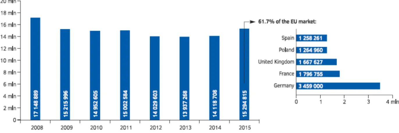
Figure 2.2 shows the amount of tons transported after the economic crisis. There has been a decrease since 2008, but the later years seem to start to recover from such crisis. In the year of 2015, of the 61% of the EU market, 3,459 million tons were from Germany alone, which are more than the 2nd and 3rd countries combined. Curiously, road freight transportation does not have such a big share of GDP in Germany as it has in the rest of the EU-28 [13], with exception of countries that are islands (UK, Ireland, Cyprus and Malta), that are unable to rely on road transportation.
By 2050, it can be expected that the demand for transport services will double in Europe [13]. Figure 2.3 shows that road transportation (blue line) is not only the most used option but the most growing method
Figure 2.2: Road freight transport in EU in the years 2008 to 2015 (in thousand tons).
Source: The Impact of Regulation of the Road Transport Sector on Entrepreneurship and Economic Growth in the European Union, Motor Transport Institute [13].
of transportation, with a trend indicating that this growth will continue in the near future (black line). A total of 3524 billion tkm goods were estimated to be transported in 2014 within the EU-28 [15]. Out of this amount, 49% was from road transportation alone.
Figure 2.3: Size of the logistics market in Europe in the years 1995 to 2014 (million ton-kilometers). Source: The Impact of Regulation of the Road Transport Sector on Entrepreneurship and Economic Growth in the European Union, Motor Transport Institute [13].
Table 2.1 shows a resume information of road freight transportation in the countries studied in this project. Portugal is a small country compared to the other 3, with a high dependency on road transporta-tion. Looking at the other 3 countries more equal in size, Spain is the most competitive internally, having more than the triple of active companies than Germany. France has the biggest turnover and Germany, although with the least share of GDP, is the country with the most volume of carriage.
Table 2.1: Road freight transport data for 2013.
Portugal Spain France Germany
Gross Domestic Product (EUR millions) 170,269 1,025,634 2,115,256 2,826,240
Turnover (EUR millions) 4,796 29,996 43,679 39,194
Share of GDP 2.8% 2.9% 2.1% 1.4%
Volume of carriage (thousand of tons) 148,177 1,124,480 1,999,869 2,938,702
Staffing (thousands) 58.8 305.8 351.8 409.9
Number of companies 8,287 108,173 37,676 35,852
Source: The Impact of Regulation of the Road Transport Sector on Entrepreneurship and Economic Growth in the European Union, Motor Transport Institute [13].
2.2
Labour
When it comes to labour legislation, Europe is facing some problems in this sector. Germany and France have minimum wage laws (MiLoG law and Loi Macron law respective) that are preventing harmonized regulation. These laws impose that a driver operating in these countries have to be paid a minimum hourly rate fixed by these countries ( C8.50/h for Germany and C9.76/h for France). This situation is allowing the possible grow of C1.4 billion/year in shadow economy with undeclared work [14]. Furthermore, companies that need to deliver or load at any of these countries will have added costs, not only the added hourly costs, but also high administrative burdens. Companies that do not deliver here but need to cross these countries are forced to rethink their strategy. Evaluating the possibility of going around, through alternative routes, that would imply different constraints (e.g.: quality of roads, more working hours due to longer routes, etc.), may have an effect on delivering times, among others, such as average speed. Many EU countries are disagreeing with these laws, invoking that these are in conflict with the freedom of the union internal market, for it disfigures the purpose of an Europe without internal borders.
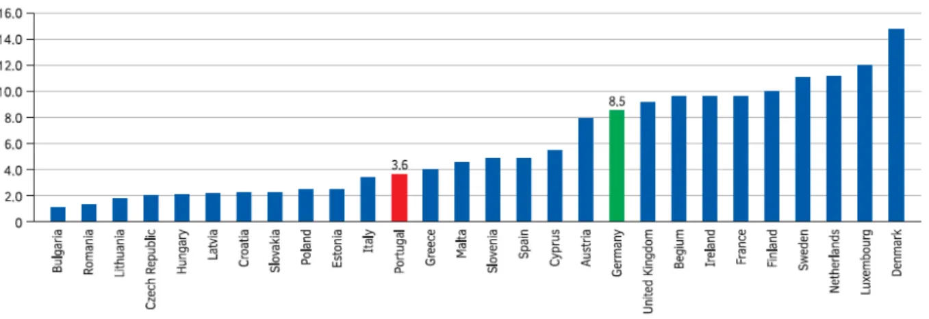
Figure 2.4 shows the minimum hourly rate for Germany (green bar), and the rest of the EU-28, including Portugal (red bar). The discrepancy is high since many countries are too far from the reality of Germany and even more from France.
France for instance, requires companies to have a local representative for inspection reasons in addition to having locally documents of payrolls, order confirmations, and workers’ contracts. Adding even more costs to outside companies.
Some benefit out of this situation: i) companies based in countries that have minimum wages higher than those of these countries are able to pay less, that is of course if their legislation allows it; ii) drivers crossing these countries have higher paychecks, for example, a driver departing from Spain with desti-nation Poland, will most likely cross both France and Germany; and ideally, iii) Germany and France, by creating a certain equality within their borders, fighting social dumping. For these laws encourage local companies to remain in these countries and not go to near countries where labour is cheaper, and also companies already on near countries will not be an unfair competition when operating in France or Germany.
Figure 2.4: Minimum hourly rate (in EUR) compared to EU Member States in 2015.
Source: The Impact of Regulation of the Road Transport Sector on Entrepreneurship and Economic Growth in the European Union, Motor Transport Institute [13].
which can be too high considering a company’s local economy. Not only that, but the drivers operating in these countries will most likely not live there, making their mandatory salaries disproportional to their economy, since these are not adjusted to their country’s purchasing power. This situation might force companies to avoid crossing these countries.
Figure 2.5 is the same information of Figure 2.4, but adjusted to each country’s purchasing power. The discrepancy is far inferior but still noticeable, especially in countries in the extremes. Denmark is still, too far from Bulgaria, in more than double.
Figure 2.5: Minimum hourly rate (in EUR) compared to EU Member States, taking into account the purchasing power equivalent to the minimum hourly rate in Germany.
Source: The Impact of Regulation of the Road Transport Sector on Entrepreneurship and Economic Growth in the European Union, Motor Transport Institute [13].
A possible alternative could be a standard minimum wage equal for the whole union. However, this would require less deviation among countries’ economies. For the countries in the extremes (Bulgaria and Denmark), it is extremely complicated to have the same minimum wage. On the other hand, uni-forming the minimum wage for one sector alone, could be a first step in the direction of a stronger, cohesive, and more socially just Europe.
3:
The Problem
The goal of a company in this business is to deliver (or pickup) an order to its destination, in time, and with the least possible costs.
A road freight transportation company has many expenses, be that with warehouses, fuel, tolls, trucks, among others. One particular expense is the expense with human resources, most, (if not all), companies have this expense. Salaries are one of the biggest costs a company can have, so it is on the interest of any company to minimize this expense. The road transportation is no different in this matter, what does differ is that drivers do not work (not only) from 8:00 to 18:00, they can work any hour of the day. Deciding when a driver works does have an impact on salaries’ expenditure, furthermore, what driver delivers what order, also has an impact, because depending on where, what route to take, and how far the destination is, has an impact on what hours the driver drives. In the end the proper allocation of drivers has a considerable impact on a company’s costs, being a problem worthy of study.
This project is focused only on the allocation of drivers ignoring everything else. Or in other words; considering everything else constant. For example, a company has a delivery to be made to a destination, (e.g.: Berlin), the truck is already loaded, and the route has already been determined. The almost all direct costs with this delivery have already been calculated, (fuel, tolls, etc.) what is left to calculate is who is going to drive this truck and what working schedules this person is going to follow. This is the focus of this work!
In road freight transportation besides salaries a company has to focus on a certain amount of rules obliged by local laws and when operating on foreign countries, also international laws. The following will be an exposure of the rules taken in consideration in this project.
3.1
Constraints
As it is expected, every activity has rules or limitations, in another word; constraints.
In this case, these constraints exist for several reasons: for fairness among competition; quality of labour for the drivers; security reasons, not only for the drivers, but also for everyone else sharing the roads with them; labour laws; etc..
Most of the constraints are permanent for the whole EU, but there are also special constraints regarding specific countries. Some are related to the country where the driver has its contract, some are applied only when present on that country.
Driving time and rest periods
The European Commission provides a common set of rules for driving and rest periods. These rules exist in order to guarantee fair competition, road safety, and drivers’ good working conditions.
These rules are:
• Daily driving period shall not exceed 9 hours, with an exemption of twice a week when it can be extended to 10 hours.
• Total weekly driving time may not exceed 56 hours and the total fortnightly1driving time may not exceed 90 hours.
• Daily rest period shall be at least 11 hours, with an exception of going down to 9 hours maximum three times a week. Daily rest can be split into 3 hours rest followed by 9 hour rest to make a total of 12 hours daily rest
• Weekly rest is 45 continuous hours, which can be reduced every second week to 24 hours. Com-pensation arrangements apply for reduced weekly rest period. Weekly rest is to be taken after six days of working, except for coach drivers engaged in a single occasional service of interna-tional transport of passengers who may postpone their weekly rest period after 12 days in order to facilitate coach holidays.
• Breaks of at least 45 minutes (separable into 15 minutes followed by 30 minutes) should be taken after 41⁄
2hours at the latest.
In this project not all rules will be applied and there are two main reasons for this.
Firstly, it is understandable that some of the rules have exceptions to allow drivers flexibility to deal with unpredictable events, such as traffic jams, accidents, flat tires, mechanical malfunctions, etc.. These are going to be ignored so that when needed, the driver has these exceptions stored as a last resort, to use outside of the driving plan in case of need. The second reason is to ease the programming, allowing a lighter program that works more efficiently. For that, is necessary that the results are produced within useful time, allowing a decision to be made.
Therefore the used rules are the following:
• Daily driving period shall not exceed 9 hours.
E.g.: If a driver works on a Monday, from the 00:00 hours of that Monday until the 24:00 hours, the total time driving may not surpass 9 hours.
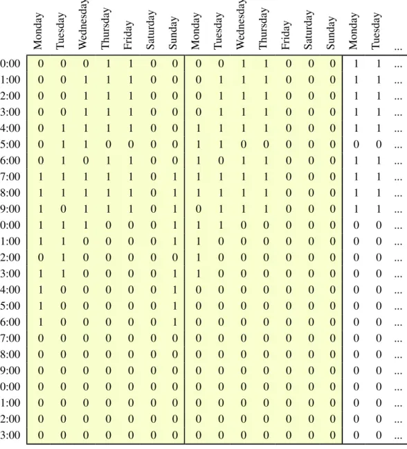
Table 3.1: Example of a driver’s weekly schedule, with focus on 9h daily constraint2.
Monday Tuesday Wednesday Thursday Friday Saturday Sunday Monday uesdayT Wednesday Thursday Friday Saturday Sunday Monday Tuesday ...
00:00 0 0 0 1 1 0 0 0 0 1 1 0 0 0 1 1 ... 01:00 0 0 1 1 1 0 0 0 1 1 1 0 0 0 1 1 ... 02:00 0 0 1 1 1 0 0 0 1 1 1 0 0 0 1 1 ... 03:00 0 0 1 1 1 0 0 0 1 1 1 0 0 0 1 1 ... 04:00 0 1 1 1 1 0 0 1 1 1 1 0 0 0 1 1 ... 05:00 0 1 1 0 0 0 0 1 1 0 0 0 0 0 0 0 ... 06:00 0 1 0 1 1 0 0 1 0 1 1 0 0 0 1 1 ... 07:00 1 1 1 1 1 0 1 1 1 1 1 0 0 0 1 1 ... 08:00 1 1 1 1 1 0 1 1 1 1 1 0 0 0 1 1 ... 09:00 1 0 1 1 1 0 1 0 1 1 1 0 0 0 1 1 ... 10:00 1 1 1 0 0 0 1 1 1 0 0 0 0 0 0 0 ... 11:00 1 1 0 0 0 0 1 1 0 0 0 0 0 0 0 0 ... 12:00 0 1 0 0 0 0 0 1 0 0 0 0 0 0 0 0 ... 13:00 1 1 0 0 0 0 1 1 0 0 0 0 0 0 0 0 ... 14:00 1 0 0 0 0 0 1 0 0 0 0 0 0 0 0 0 ... 15:00 1 0 0 0 0 0 1 0 0 0 0 0 0 0 0 0 ... 16:00 1 0 0 0 0 0 1 0 0 0 0 0 0 0 0 0 ... 17:00 0 0 0 0 0 0 0 0 0 0 0 0 0 0 0 0 ... 18:00 0 0 0 0 0 0 0 0 0 0 0 0 0 0 0 0 ... 19:00 0 0 0 0 0 0 0 0 0 0 0 0 0 0 0 0 ... 20:00 0 0 0 0 0 0 0 0 0 0 0 0 0 0 0 0 ... 21:00 0 0 0 0 0 0 0 0 0 0 0 0 0 0 0 0 ... 22:00 0 0 0 0 0 0 0 0 0 0 0 0 0 0 0 0 ... 23:00 0 0 0 0 0 0 0 0 0 0 0 0 0 0 0 0 ...
worked ≤ 9h total per day
2
A ”1” in a cell represents that 1 hour was driven from that cell’s name to the next cell’s name. E.g.: in the 1stcolumn (Monday), the cell with name 07:00 has a ”1”, this means that the driver drove from the 07:00 hours to the 08:00 hours. A ”0” on the other hand means that in that hour the driver was stopped. A better explanation will be provided in chapter 4.
• Total fortnightly driving time may not exceed 90 hours.
E.g.: Similar to the 9 hours per day limit; a driver that has been driving from the 1stof the month,
(from the 00:00 hours of Monday), until the 14thof the same month, (the 24:00 hours of Sunday), cannot have driven more than a total of 90 hours for that interval. The same from the 2nd of the month, (from the 00:00 hours of Tuesday), until the 15th of the same month, (the 24:00 hours of Monday). I.e.: In a period of 14 consecutive days a driver cannot exceed a total of 90 worked hours.
Table 3.2: Example of a driver’s weekly schedule, with focus on 90h weekly constraint.
Monday Tuesday Wednesday Thursday Friday Saturday Sunday Monday uesdayT Wednesday Thursday Friday Saturday Sunday Monday Tuesday ...
00:00 0 0 0 1 1 0 0 0 0 1 1 0 0 0 1 1 ... 01:00 0 0 1 1 1 0 0 0 1 1 1 0 0 0 1 1 ... 02:00 0 0 1 1 1 0 0 0 1 1 1 0 0 0 1 1 ... 03:00 0 0 1 1 1 0 0 0 1 1 1 0 0 0 1 1 ... 04:00 0 1 1 1 1 0 0 1 1 1 1 0 0 0 1 1 ... 05:00 0 1 1 0 0 0 0 1 1 0 0 0 0 0 0 0 ... 06:00 0 1 0 1 1 0 0 1 0 1 1 0 0 0 1 1 ... 07:00 1 1 1 1 1 0 1 1 1 1 1 0 0 0 1 1 ... 08:00 1 1 1 1 1 0 1 1 1 1 1 0 0 0 1 1 ... 09:00 1 0 1 1 1 0 1 0 1 1 1 0 0 0 1 1 ... 10:00 1 1 1 0 0 0 1 1 1 0 0 0 0 0 0 0 ... 11:00 1 1 0 0 0 0 1 1 0 0 0 0 0 0 0 0 ... 12:00 0 1 0 0 0 0 0 1 0 0 0 0 0 0 0 0 ... 13:00 1 1 0 0 0 0 1 1 0 0 0 0 0 0 0 0 ... 14:00 1 0 0 0 0 0 1 0 0 0 0 0 0 0 0 0 ... 15:00 1 0 0 0 0 0 1 0 0 0 0 0 0 0 0 0 ... 16:00 1 0 0 0 0 0 1 0 0 0 0 0 0 0 0 0 ... 17:00 0 0 0 0 0 0 0 0 0 0 0 0 0 0 0 0 ... 18:00 0 0 0 0 0 0 0 0 0 0 0 0 0 0 0 0 ... 19:00 0 0 0 0 0 0 0 0 0 0 0 0 0 0 0 0 ... 20:00 0 0 0 0 0 0 0 0 0 0 0 0 0 0 0 0 ... 21:00 0 0 0 0 0 0 0 0 0 0 0 0 0 0 0 0 ... 22:00 0 0 0 0 0 0 0 0 0 0 0 0 0 0 0 0 ... 23:00 0 0 0 0 0 0 0 0 0 0 0 0 0 0 0 0 ...
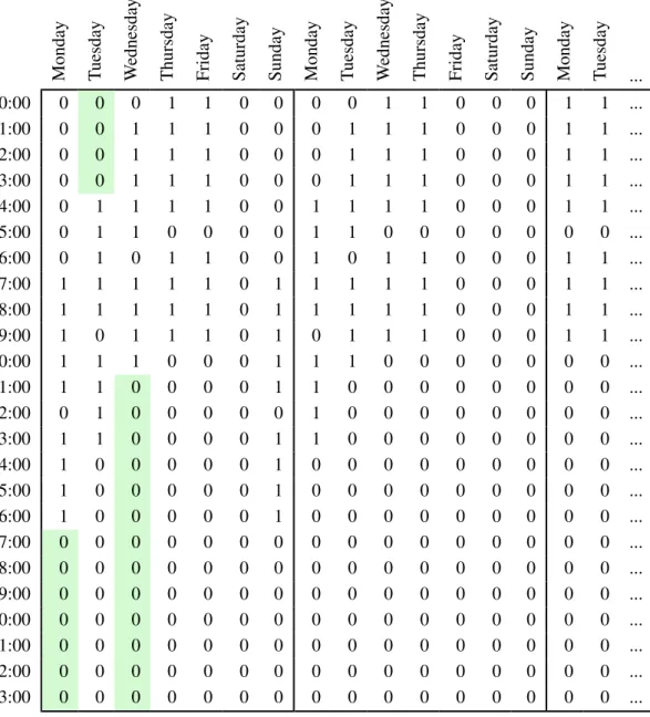
• Daily rest period shall be of at least 11 uninterrupted hours.
The European Commission rules are not clear about the continuity of the daily rest period, it is implied, but there is some room for ambiguity. If the 11 hours rest wouldn’t need to be necessarily continuous, that would mean that a driver could drive for 1 hour and then rest for 1 hour, then drive for 1 hour, rest 1 hour gain, and so on, for the whole day. There are other reasons to consider the continuity of this break that will be better explained later in this chapter.
Table 3.3: Example of a driver’s weekly schedule, with focus on 11h daily rest constraint.
Monday Tuesday Wednesday Thursday Friday Saturday Sunday Monday uesdayT Wednesday Thursday Friday Saturday Sunday Monday Tuesday ...
00:00 0 0 0 1 1 0 0 0 0 1 1 0 0 0 1 1 ... 01:00 0 0 1 1 1 0 0 0 1 1 1 0 0 0 1 1 ... 02:00 0 0 1 1 1 0 0 0 1 1 1 0 0 0 1 1 ... 03:00 0 0 1 1 1 0 0 0 1 1 1 0 0 0 1 1 ... 04:00 0 1 1 1 1 0 0 1 1 1 1 0 0 0 1 1 ... 05:00 0 1 1 0 0 0 0 1 1 0 0 0 0 0 0 0 ... 06:00 0 1 0 1 1 0 0 1 0 1 1 0 0 0 1 1 ... 07:00 1 1 1 1 1 0 1 1 1 1 1 0 0 0 1 1 ... 08:00 1 1 1 1 1 0 1 1 1 1 1 0 0 0 1 1 ... 09:00 1 0 1 1 1 0 1 0 1 1 1 0 0 0 1 1 ... 10:00 1 1 1 0 0 0 1 1 1 0 0 0 0 0 0 0 ... 11:00 1 1 0 0 0 0 1 1 0 0 0 0 0 0 0 0 ... 12:00 0 1 0 0 0 0 0 1 0 0 0 0 0 0 0 0 ... 13:00 1 1 0 0 0 0 1 1 0 0 0 0 0 0 0 0 ... 14:00 1 0 0 0 0 0 1 0 0 0 0 0 0 0 0 0 ... 15:00 1 0 0 0 0 0 1 0 0 0 0 0 0 0 0 0 ... 16:00 1 0 0 0 0 0 1 0 0 0 0 0 0 0 0 0 ... 17:00 0 0 0 0 0 0 0 0 0 0 0 0 0 0 0 0 ... 18:00 0 0 0 0 0 0 0 0 0 0 0 0 0 0 0 0 ... 19:00 0 0 0 0 0 0 0 0 0 0 0 0 0 0 0 0 ... 20:00 0 0 0 0 0 0 0 0 0 0 0 0 0 0 0 0 ... 21:00 0 0 0 0 0 0 0 0 0 0 0 0 0 0 0 0 ... 22:00 0 0 0 0 0 0 0 0 0 0 0 0 0 0 0 0 ... 23:00 0 0 0 0 0 0 0 0 0 0 0 0 0 0 0 0 ...
• Weekly rest is of at least 45 continuous hours.
E.g.: Between the 00:00 hours of Monday until the 24:00 hours of Sunday (of the same week), a driver has to have at least 1 interval of at least 45 uninterrupted resting hours. This applies to every set of 7 straight days. E.g.: From 00:00 hours of Monday to the 24:00 hours of Sunday, then the same to the 00:00 hours of Tuesday to the 24:00 hours of next Monday, and so on.
Table 3.4: Example of a driver’s weekly schedule, with focus on 45h weekly rest constraint.
Monday Tuesday Wednesday Thursday Friday Saturday Sunday Monday uesdayT Wednesday Thursday Friday Saturday Sunday Monday Tuesday ...
00:00 0 0 0 1 1 0 0 0 0 1 1 0 0 0 1 1 ... 01:00 0 0 1 1 1 0 0 0 1 1 1 0 0 0 1 1 ... 02:00 0 0 1 1 1 0 0 0 1 1 1 0 0 0 1 1 ... 03:00 0 0 1 1 1 0 0 0 1 1 1 0 0 0 1 1 ... 04:00 0 1 1 1 1 0 0 1 1 1 1 0 0 0 1 1 ... 05:00 0 1 1 0 0 0 0 1 1 0 0 0 0 0 0 0 ... 06:00 0 1 0 1 1 0 0 1 0 1 1 0 0 0 1 1 ... 07:00 1 1 1 1 1 0 1 1 1 1 1 0 0 0 1 1 ... 08:00 1 1 1 1 1 0 1 1 1 1 1 0 0 0 1 1 ... 09:00 1 0 1 1 1 0 1 0 1 1 1 0 0 0 1 1 ... 10:00 1 1 1 0 0 0 1 1 1 0 0 0 0 0 0 0 ... 11:00 1 1 0 0 0 0 1 1 0 0 0 0 0 0 0 0 ... 12:00 0 1 0 0 0 0 0 1 0 0 0 0 0 0 0 0 ... 13:00 1 1 0 0 0 0 1 1 0 0 0 0 0 0 0 0 ... 14:00 1 0 0 0 0 0 1 0 0 0 0 0 0 0 0 0 ... 15:00 1 0 0 0 0 0 1 0 0 0 0 0 0 0 0 0 ... 16:00 1 0 0 0 0 0 1 0 0 0 0 0 0 0 0 0 ... 17:00 0 0 0 0 0 0 0 0 0 0 0 0 0 0 0 0 ... 18:00 0 0 0 0 0 0 0 0 0 0 0 0 0 0 0 0 ... 19:00 0 0 0 0 0 0 0 0 0 0 0 0 0 0 0 0 ... 20:00 0 0 0 0 0 0 0 0 0 0 0 0 0 0 0 0 ... 21:00 0 0 0 0 0 0 0 0 0 0 0 0 0 0 0 0 ... 22:00 0 0 0 0 0 0 0 0 0 0 0 0 0 0 0 0 ... 23:00 0 0 0 0 0 0 0 0 0 0 0 0 0 0 0 0 ...
• Breaks of at least 1 hour after a maximum of 5 straight hours of work.
E.g.: If a driver has started to work at 07:00 hours, by the 12:00 hours, if it hasn’t had a break within this interval, it has to forcibly have one now. This break can be of just 1 hour, or more, but forcibly, it has to be of at least 1 hour.
Table 3.5: Example of a driver’s weekly schedule, with focus on 5h continuous work constraint.
Monday Tuesday Wednesday Thursday Friday Saturday Sunday Monday uesdayT Wednesday Thursday Friday Saturday Sunday Monday Tuesday ...
00:00 0 0 0 1 1 0 0 0 0 1 1 0 0 0 1 1 ... 01:00 0 0 1 1 1 0 0 0 1 1 1 0 0 0 1 1 ... 02:00 0 0 1 1 1 0 0 0 1 1 1 0 0 0 1 1 ... 03:00 0 0 1 1 1 0 0 0 1 1 1 0 0 0 1 1 ... 04:00 0 1 1 1 1 0 0 1 1 1 1 0 0 0 1 1 ... 05:00 0 1 1 0 0 0 0 1 1 0 0 0 0 0 0 0 ... 06:00 0 1 0 1 1 0 0 1 0 1 1 0 0 0 1 1 ... 07:00 1 1 1 1 1 0 1 1 1 1 1 0 0 0 1 1 ... 08:00 1 1 1 1 1 0 1 1 1 1 1 0 0 0 1 1 ... 09:00 1 0 1 1 1 0 1 0 1 1 1 0 0 0 1 1 ... 10:00 1 1 1 0 0 0 1 1 1 0 0 0 0 0 0 0 ... 11:00 1 1 0 0 0 0 1 1 0 0 0 0 0 0 0 0 ... 12:00 0 1 0 0 0 0 0 1 0 0 0 0 0 0 0 0 ... 13:00 1 1 0 0 0 0 1 1 0 0 0 0 0 0 0 0 ... 14:00 1 0 0 0 0 0 1 0 0 0 0 0 0 0 0 0 ... 15:00 1 0 0 0 0 0 1 0 0 0 0 0 0 0 0 0 ... 16:00 1 0 0 0 0 0 1 0 0 0 0 0 0 0 0 0 ... 17:00 0 0 0 0 0 0 0 0 0 0 0 0 0 0 0 0 ... 18:00 0 0 0 0 0 0 0 0 0 0 0 0 0 0 0 0 ... 19:00 0 0 0 0 0 0 0 0 0 0 0 0 0 0 0 0 ... 20:00 0 0 0 0 0 0 0 0 0 0 0 0 0 0 0 0 ... 21:00 0 0 0 0 0 0 0 0 0 0 0 0 0 0 0 0 ... 22:00 0 0 0 0 0 0 0 0 0 0 0 0 0 0 0 0 ... 23:00 0 0 0 0 0 0 0 0 0 0 0 0 0 0 0 0 ...
worked ≤ 5h continuous work
Since the program is designed to work with units of 1 hour, it isn’t possible to work with 41⁄2hours or
breaks of less than 1 hour. It is then rounded to a maximum of 5 hours and breaks of 1 hour. This is easily convertible by adjusting the program to work with fragments of hour instead of 1 hour units, (i.e.:
1⁄
The 56 hours per week limit is ignored due to the fact that it is impossible to exceed this without ex-ceeding the 9 hour per day limit or the weekly rest of 45 continuous hours. If on a week, a driver would drive every day (9h per day), in the end of the week, it would have driven a total of 64 hours. But this would exceed the 45h rest limit. Assuming that a driver could drive the first 9 hours of a day (from 00:00 to 09:00), continuously, and the last 9 hours of the next day (15:00 to 24:00), it would only be a total of 30 continuous rest hours. To respect the 45h constraint, a driver can, at best, rest for a full day (it is impossible not to, since 45h of mandatory rest will always include a full day), continue to rest the next day for 21 hours (making it 45h), and then drive the last 3 hours of that day3. But this means that in a period of 2 days the driver has driven only 3 hours, adding this to the remaining 5 days of the week, sums to a total of 3 hours plus 5 times 9 hours, i.e.: 48 worked hours on that week.
Table 3.6: Example 1 of the 56h constraint redundancy.
Monday Tuesday Wednesday Thursday Friday Saturday Sunday ...
00:00 0 0 1 1 1 1 1 ... 01:00 0 0 1 1 1 1 1 ... 02:00 0 0 1 1 1 1 1 ... 03:00 0 0 1 1 1 1 1 ... 04:00 0 0 1 1 1 1 1 ... 05:00 0 0 0 0 0 0 0 ... 06:00 0 0 1 1 1 1 1 ... 07:00 0 0 1 1 1 1 1 ... 08:00 0 0 1 1 1 1 1 ... 09:00 0 0 1 1 1 1 1 ... 10:00 0 0 0 0 0 0 0 ... 11:00 0 0 0 0 0 0 0 ... 12:00 0 0 0 0 0 0 0 ... 13:00 0 0 0 0 0 0 0 ... 14:00 0 0 0 0 0 0 0 ... 15:00 0 0 0 0 0 0 0 ... 16:00 0 0 0 0 0 0 0 ... 17:00 0 0 0 0 0 0 0 ... 18:00 0 0 0 0 0 0 0 ... 19:00 0 0 0 0 0 0 0 ... 20:00 0 0 0 0 0 0 0 ... 21:00 0 1 0 0 0 0 0 ... 22:00 0 1 0 0 0 0 0 ... 23:00 0 1 0 0 0 0 0 ...
≥ 45h of continuous rest per week
Another, and better way, would be to completely stop for a full day, 24h of rest, and split the remaining needed hours to complete the total of 45h rest, among the previously and following days. I.e.: a driver drives the first 9 hours of a day (even ignoring the mandatory rest of 1 hour per 5 continuous hours of work), rests the remaining 15 hours of that day. Rests completely the next day, (making it a total of 39 already rested hours). And on the third day, rests the missing 6 hours, and then works 9 hours. This would allow a driver to work 18 hours in a period of 3 days, while performing the mandatory 45h weekly rest. Adding the remaining 4 days of work, would mean a total of 9 worked hours in 6 days, that are 54 hours, less that 56 hours. Even if driving to a limit of 10 hour per day, 2 times a week, it wouldn’t be exceeded. Which makes it redundant hence being ignored.
Table 3.7: Example 2 of the 56h constraint redundancy.
Monday Tuesday Wednesday Thursday Friday Saturday Sunday ...
00:00 1 0 0 1 1 1 1 ... 01:00 1 0 0 1 1 1 1 ... 02:00 1 0 0 1 1 1 1 ... 03:00 1 0 0 1 1 1 1 ... 04:00 1 0 0 1 1 1 1 ... 05:00 1 0 0 0 0 0 0 ... 06:00 1 0 1 1 1 1 1 ... 07:00 1 0 1 1 1 1 1 ... 08:00 1 0 1 1 1 1 1 ... 09:00 0 0 1 1 1 1 1 ... 10:00 0 0 1 0 0 0 0 ... 11:00 0 0 0 0 0 0 0 ... 12:00 0 0 1 0 0 0 0 ... 13:00 0 0 1 0 0 0 0 ... 14:00 0 0 1 0 0 0 0 ... 15:00 0 0 1 0 0 0 0 ... 16:00 0 0 0 0 0 0 0 ... 17:00 0 0 0 0 0 0 0 ... 18:00 0 0 0 0 0 0 0 ... 19:00 0 0 0 0 0 0 0 ... 20:00 0 0 0 0 0 0 0 ... 21:00 0 0 0 0 0 0 0 ... 22:00 0 0 0 0 0 0 0 ... 23:00 0 0 0 0 0 0 0 ...
≥ 45h of continuous rest per week
Portuguese Law
Table 3.8: Example of the exploit of the EU rules compared to the addition of the Portuguese Law. Driver 1 Driver 2 2017-01-01 03:00 0 1 2017-01-01 04:00 0 1 2017-01-01 05:00 0 1 2017-01-01 06:00 0 1 2017-01-01 07:00 0 1 2017-01-01 08:00 0 0 2017-01-01 09:00 0 1 2017-01-01 10:00 0 1 2017-01-01 11:00 0 1 2017-01-01 12:00 0 1 2017-01-01 13:00 0 0 2017-01-01 14:00 1 0 2017-01-01 15:00 1 0 2017-01-01 16:00 1 0 2017-01-01 17:00 1 0 2017-01-01 18:00 1 0 2017-01-01 19:00 0 0 2017-01-01 20:00 1 0 2017-01-01 21:00 1 0 2017-01-01 22:00 1 0 2017-01-01 23:00 1 0 2017-01-02 00:00 1 1 2017-01-02 01:00 0 1 2017-01-02 02:00 1 1 2017-01-02 03:00 1 1 2017-01-02 04:00 1 1 2017-01-02 05:00 1 0 2017-01-02 06:00 1 1 2017-01-02 07:00 0 1 2017-01-02 08:00 1 1 2017-01-02 09:00 1 1 2017-01-02 10:00 1 0
≥ 11h∗ = (11h of rest per day + P T Law) worked ≤ 5h continuous work
Since in this project it is considered a Portuguese based company, the drivers are covered by Portuguese law, and it decrees that a driver (and any other worker) cannot work 2 consecutive driving periods (of 9 hours) without an interrupted rest period of 11 continuous hours, which in this case means that a driver
can at best, work a total of 18 hours in a period of 31 hours. In Table 3.8 Driver 1 is exploiting this loophole, where Driver 2 is according to the Portuguese Law.
Given the European Union rules, a driver would never be able to drive 18 hours in the same day. However, a driver could drive two consecutive driving periods, if these periods would take place in the end of a day and on the immediate beginning of the next day. I.e.: The driver starts to work at 14:00 of Monday and finishes the day’s shift at the 24:00 of the same day. Later at 01:00 of Tuesday, the driver starts to work again, finishing that day’s shift at 11:00, making 18 hours of driving in less than 24 hours. This situation is feasible by European rules, it is a loop hole, since the rules mention daily driving, but not the day as a set of 24 continuous hours. It would be a tempting exploit of the rules, particularly regarding destinations within small distances. However, the Portuguese law forbids this, and to incorporate such law, the daily rest of 11 hours will be adjusted. Instead of considering periods of time as a singular civil day. A day, in this case, will be taken as a continuous sequence of 24 hours to make sure that a driver has 11 hours of uninterrupted rest after, or before, working a complete shift.
Locations
Some countries have their own specific driving constraints. Most of these constraints have to do with cargo, which is not a subject of study in this project. The constraints to have into account are related to weekends and holidays, namely in France and Germany. In France, it is not allowed to drive between the 22:00 of Saturday until the 22:00 of Sunday. The same applies to holidays and the day immediately before, e.i.: no driving allowed between the 22:00 of the day before a holiday and the 22:00 of the holiday.
Germany has similar constraints. It isn’t allowed to transport goods through land between the 00:00 and 22:00 on Sundays and holidays.
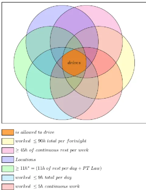
Figure 3.1 gives a visual idea of when the driver is allowed to drive, where each circumference represents one of the used restrictions. Only when within all restrictions is the driver able to drive.
Figure 3.1: Representative diagram of constraints. A driver can drive if within the constraints. (Disk’s dimensions are not representative of the constraints’ grasp).
3.2
Objectives
The goal of this project it to improve the allocation of drivers in order to have minimum global costs, satisfying the demand while reaching the destinations within an acceptable time window.
Time and costs are critical when allocating drivers. When it comes to costs the reasons are very straight-forward; less direct costs mean more profit, be that by improving margins, practicing more competitive prices, a mix of both, or even using these savings in research and development. A more efficient com-pany is a more competitive comcom-pany. The proper allocation of drivers affects a comcom-pany costs, not only deciding what driver must take the deliver, but also, when it is the best moment to depart, and what are the best hours to work, so that the restrains are respected but that the company does not endure in unnecessary costs. For example; it’s 20:00 on a Monday and there is an order to be delivered to a 25 hours far destination. If a driver starts to drive now, it will drive the remaining 4 hours of Monday, drive 9 hours on Tuesday, plus 9 hours on Wednesday, and it reaches its destination on Thursday, at beast, at 3:00. Allocating the driver this way would incur in a direct cost of C133.75, (assuming that a driver is payed C5 per hour, and that in nightly hours it has an increase of 25%). If the company decides to wait and only let the driver start on the next morning at 8:00, the driver will reach its destination also on Thursday at the 15:00, for a total cost of C125. The driver can deliver the order in the same day with a difference of C8.75. It may not seem like much, but when scaling for a total number of delivers a driver does per year, and considering that a company has many drivers, a small amount such as this makes a big difference.
Time may not be so straightforward when it comes to its importance but it is also of great relevance in the freight transport business. Every client needs its orders in time, a company that takes longer than the competition to deliver, is a company that stays behind. It is important for a company’s image, to be reliable and efficient. A company needs to deliver within what is the average market delivery time, but if it can do better, then it is more appealing for its customers. Allocating the right driver can make all the difference. Like in the example above, there is an order to be delivered to a 25 hours far destination, and there are two possible drivers. The 1stdriver is a driver that has a cumulative sum of 75 worked hours in the last 12 days, the 2nddriver is a driver that for the same previously 12 days, has a cumulative sum of 65 worked hours. If the company chooses to allocate the 1stdriver, it will drive the first day for 9 hours, reaching a total of 84 hours in 13 days, and on the following day it will reach the limit of 90 hours per fortnight with 6 hours driven, being forced to stop for the rest of the day. Since it has 10 hours left to reach its destination and knowing that it can only drive a total of 9 hour per day, this means that the 1st driver will take 4 days to reach this destination. The 2nddriver on the other hand, can drive 9 hours on the first day, plus another 9 hours on the following day, and on the 3rd day it will reach its destination after driving for 7 hours. In this example, allocating the right drive has a difference of a day and that can make a huge difference for the client.
Direct costs, and arriving costs (or indirect costs) are important individually, but they can also be im-proved together. In a pool of available drivers it is possible to have multiple drivers arriving at the destination in the same moment at different costs. The opposite is also possible, for the same cost, mul-tiple drivers can reach the destination in different moments. Reaching the destination as soon as possible with the minimum possible cost is the ideally situation, when this is not possible it is required to define what weights the most, the arriving moment or the cost? Is it worth allocating a driver that arrives an
hour late if that means saving C20? Arriving a full day sooner is worth allocating a driver that will have an higher cost of C10?
The all drivers’ allocation or even just a driver’s schedule has a large amount of feasible solutions that respect these constraints. Optimizing a driver’s schedule resorting to operations research, in specific, integer programming, would take a considerable amount of computer processing, which translates into many hours of calculations until the optimum solution would be reached. The farther the destination the more time would take to achieve the best solution. Allocating the whole drivers’ fleet this way would just increase this situation exponentially.
To avoid this, it was used a methodology focused on the goal of making a driver reach its destination as fast as possible, respecting the existing constraints. Once this information is calculated for every driver on the fleet, it was then optimized the allocation using now operations research.
4:
Methodology
A program was developed in order to help in the decision of allocating drivers to the different destina-tions. The goal of this program was to create different schedules for all the available drivers. Where a driver departs as soon as it is able, driving every day it can, and as soon as it can on each day, until the destination is reached. Then the program calculates the same but departing 1 hour later, and then 1 hour more, and so on, for as many times (hours) as the manager decides it is important to analyze. For example, a driver can depart as soon as 03:00, the second schedule will be with the driver departing at 04:00, and the third at 05:00, and so on. Then this process is repeated for every destination and every driver.
After all this information has been calculated, begins the allocation optimization. Where it is calculated the cost per each schedule, both direct costs with drivers hourly rates, and indirect costs with arriving moments, and then according to the demand, it is optimized the best global allocation that satisfies this demand with minimal costs.
4.1
Specifications
All software used in this project is open source, with exception of Microsoft’s Excel. These are; R, R-studio, QGIS and LibreOffice. The date format used is the indicated by the ISO norm 8601. The average speed and the routes/roads taken to reach the destination are consider as inputs. The timezone used is the western European time zone UTC+00:00. The difference in time zones is ignored for what is important is how long the driver is driving, regardless of what the local clocks present.
The departing city is Lisbon and there will be 3 possible destinations; Madrid, Paris and Berlin. Once a driver, allocated to a destination, reaches it, it will immediately start to travel back. It will be ignored any time spent with loading and unloading the trailer. It is assumed that the trailers are timely loaded for the drivers and that a driver, upon arriving, switches trailers and keeps on moving (if eligible to do so). This is ignored for several reasons. Usually the drivers are not the ones who load or unload the trailers, this work is generally accomplished by the warehouse workers. Another reason, and most importantly, is that it is not wise to define a rule that forces a driver to remain in a destination for an extra hour, since it is not unusual for a driver to have to be stopped due to its own constraints. Therefore there would be many occasions where the driver would have its trailer unloaded and reloaded, ready for the trip back while resting. But in other occasions it would have to be forced to stay idle, despite the fact that it could be on the move already. It would be possible to solve this without much problem, but that would not make the program necessarily more realistic, especially considering that a switch of trailers is quite realistic in a company that has a high frequency of shipments. This can, however, be added to the heuristic later if eventually wanted or needed.
Cabotage1was ignored in this project. Adding this would increase the level of complexity of the problem, requiring that the program would have to calculate more information. For example, a driver delivers an order from Lisbon to Berlin and upon returning brings a delivery from Berlin to Paris, and then another delivery from Paris to Madrid. This would require an advance adjustment of dates, for pickups and dropouts, and an adjustment to have a driver in a compatible route when those delivers exist. It is possible that the program can be adjust to this from of activity, although that surpass the environment of this project, and for now, it is ignored.
4.2
Inputs
For the program to function properly it needs to adjust to the company’s reality, to do so, some inputs are required. This is a situation of continuity. There is a recent pass that has to be taken into consideration, namely, the driver’s driving history.
Other information that the program needs beforehand are the lists of holidays for each of the countries where the company operates. These are of significant impact, needed for the driving constraints, and for the calculation of costs.
Another indispensable information are the destinations’ distances. The program needs to know where to send the drivers, or in the program’s understanding, how many hours the driver has to drive to reach its destination.
On the financial side of things, the program needs to know how are the costs calculated. I.e.: what is the hourly rate for a driver to drive on a particular hour, in order to present the total cost per driver.
A final input necessary is the interval of days for the program to work with. The program needs to know where is working, in time, so that it can take into consideration the proper driver’s history, the holidays, and the interval limit of time to work.
Holidays
The Holidays’ information is something that can be updated only once - in the beginning of every year. Most holidays are stationary, and although they are all predictable, some are harder to calculate, as it is the case with Easter and other religious holidays. Not to mention that for political, economical or social reasons, holidays may be added or excluded as such.
The holidays to have into consideration are only the holidays of countries where the company operates, and even so, not all countries’ holidays may have to be considered. Many countries have regional holi-days that may not affect the company, and other countries’ holiholi-days don’t have any impact at all, such is the case of Spain.
As mentioned in chapter 3, France and Germany have driving constraints that are associated to these countries’ holidays. Without knowing when these holidays occur, the program would be at fault, creating inadequate schedules, disrespecting these countries’ rules, leaving the company with unnecessary issues, with the possibility of incurring in unnecessary expenses with fines for example.
Another reason why holidays are an important input has to do with the company’s head quarters being in Portugal, and the drivers being covered by Portuguese law. This means that driver’s variables pays are influenced by holidays in Portugal.
Costs
In order to accurately calculate a driver’s schedules cost, it is necessary to know how much a driver’s hourly rate is. To that, it is also required to add the information regarding night hourly rates, holiday rates and weekend rates. For this project, the following rates were required: the Portuguese Labour Law rates; and eventually other rates could be needed, such as, different basic hourly rates per drive. E.g.: A driver that has been with the company for several years might have a higher hourly rate than others. The costs with trucks, regarding maintenance, fuel, tolls or any other expenses are ignored. It is assumed that these costs are constant with the destination. The costs of shipment from Lisbon to Berlin are greater than shipping from Lisbon to Madrid particularly with fuel and tolls, but that is not taken in consideration, since the destinations will not be competing among themselves. The focus is on satisfying every destination’s need.
It will be assumed that the drivers have a fixed wage and that they are paid an extra over worked hours. By default a driver is payed 5 units per worked hour. I.e.: if a driver is on route but it is idle, it it won’t get paid. If on the other hand, it is driving, then it receives, (by default) 5 units per hour. As previously mentioned on chapter 3, the drivers are covered by Portuguese law. This states that the worked hours on particular cases have a percentage added to the default value. When driving at nigh hours, drivers get an extra 25% over the standard value, making it a 6.25 units. A night hour is an hour that is contained in the interval from 22:00 of a day to the 07:00 of the following day, inclusive. On the weekends drivers get payed an extra 50% (7.50 units). And on Holidays an 75% extra. All of this is considered in Portuguese time zone, as if the driver is in Portuguese territory. E.g.: a driver is driving in Germany, and the local time is 22:00 (UTC+01:00), the driver will not be paid as a night hour, since in Portugal it is 21:00 (UTC+00:00). On the other hand, if a driver is driving at 07:00 local time and it is still 06:00 in Portugal, then the driver is paid as a night hour. The same is applied to weekends and holidays. These add values are non cumulative, prevailing the highest values. E.g.: A driver is working on a holiday, which happens to be on a weekend and at night, then the driver only gets paid the extra 75%, not a cumulative 150% (25% + 50% + 75%).
Arriving to a destination at different possible times has to be convertible to a mensurable meaning. In order to do so, it is considered the soonest moment of arrival to a destination as a 0 cost. Arriving 1 hour later, will be considered as 1 unit of costs, 2 hours later, 2 units of costs, an so on. E.g.: a driver can arrive the soonest to Paris at 2017-01-31 05:00, this will be considered to cost 0 units. This is the standard arriving moment for this destination. An alternative arriving moment, such as 2017-02-02 00:00 will be converted to 43 units of cost, because the driver arrives 43 hours later.
The MiLoG and Loi Macron laws are ignored, for it was not clear how this laws are applied in combina-tion with the Portuguese Labour Law. Te loss of this informacombina-tion does not have a high impact on the goal of this project, and it can easily be added to the costs’ calculation in a future version of the program. Different solutions would possible be presented, but the demand would still need to be satisfied, and the countries in question would not be avoided in any way since routes are not a subject of study here. Regardless, the program is able to incorporate these laws if wanted.
Destinations
In order for the program to calculate the schedule for a driver, it needs to know what this driver’s desti-nation is. For the program, a destidesti-nation is a total number of working hours, so, it is then necessary to tell the program how many hours it takes to reach each destination.
To calculate a destination’s length in hours, it was taken into consideration the average speed of 80 kilometers per hour. Therefore, a distance of a 1,000 km is interpreted as 13 driving hours.
Routes are not taken into account because it is considered that there aren’t many significant available options, i.e.: options that actually have an impact on this type of project. Obviously there are many alternative routes that reach the same destination, but they are hardly ever going to avoid a main freeway that consumes most of the traveling time. When it comes to national roads there are plenty of alternatives, and many of which might be important due to several reasons, such as road traffic depending on when they are traveled; constructions; road repairs; etc.. That, however, is beyond the scope of this project. It is just accepted that the routes are the best in a long term and that on average, regardless of the route, a driver takes a given amount of time to reach its destination and it is based on that amount that the program functions.
Since for this project those statistics were not available, it was calculated the time a driver needs to reach its destination by dividing the total distance in kilometers by the average speed mentioned.
Driver’s history
To know if a driver is eligible to drive, respecting the mentioned constraints, it is indispensable to have the information regarding drivers’ history of previously worked hours. The farthest this history has to go is the previously fortnight2. Farther information is not necessary, but this is, in order to respect constraints like: the 90 hours limit per fortnight, the 45 hours rest per week, and, the 11 hours rest per daily shift. Even if a driver is technically new and has no driving history it has to have this information available. In this case it just so happens to be a fortnight of comply rest. Same goes for drivers returning from holidays. The program will not work without this information.
Time window
Finally and more trivially, the program requires a time window to be defined. The starting day (and hour) must be equal to the first day of the inputted drivers’ history, and the ending day must be far enough for the program to work. I.e.: the last fortnight plus enough days for the driver to return from its destination, with days to spare. Having more days than exactly needed will not have significant influence on the program’s performance, since the program stops as soon as the driver has returned. On the other hand, having insufficient days will prevent the program from working properly.
This input is not an important part of the problem as much as a result of the design of the program. The program can be improved in order not to be dependable of the user to calculate this information, since it could probably just estimate the length of this time window, by looking at the available drivers’ history ending date, and then adding more days/hours as it would be needed during the calculation of the schedules.
2
To be precise only the previously 13 days are actually needed, since the 14thday will be the currently day being analyzed by the program.
This, however, would require more developing time and since it didn’t have much impact on the end result, it was ignored. On the other hand, this allows testing the program for different time windows and other aspects, by giving the user more control.
4.3
Heuristic
For a driver’s schedule for only 1 day, from the 00:00 to the 24:00 hours, assuming that this driver drives a total of 9 hours, and that it does not drive more than 5 straight hours, there are over a 1.000.000 feasible solutions3. To reach THE optimum solution for minimum costs for this particular day, it would require the use of integer programming, which is usually a slow process due to its characteristics. The more feasible solutions and more constraints, the slower the optimization is, in the previous example it was ignored the fact that a driver can drive less than 9 hours in a day, and all other constraints used in this project4, meaning that the number of admissible solutions would be even bigger. To optimize (minimizing costs) the hole allocation of every admissible driver, satisfying the demand and respecting every constrain while using integer programming would take a long time. If this process would start and at the same time a driver would depart for a destination, this driver would have return before the process would be concluded. To avoid this time consuming, it was built an heuristic that finds A solution, a called ”greedy heuristic”, that is designed to make the driver drive every time it is eligible until the destination is reached, (and then return), ignoring costs. This is calculated for several different departing moments per driver, and only after all drivers have all this calculated is then used integer programming for the optimization for minimum costs, with a considerable less amount of data to be processed in the optimization, gaining time at the expense of missing the optimum solution, but finding a solution that is useful. The used heuristic is a simple one that can be improved, but the more rules the heuristic has the more likely it is to be slower. However, it is possible to have more rules that compensate their existence by avoiding unnecessary calculations that translate in better overall performance.
By default the driver is stopped (using binary; 0). The program analyses one hour at a time. It asks itself ”can I drive in this hour?”, and if no constraints forbid it, then the driver drives that given hour5(in binary; 1). And so on, until a constraint forbids it, or the destination is reached. It is also designed so it doesn’t waste too much computation with a period of time that isn’t going to be available soon. I.e.: if the driver has just finished a daily period of driving, there is no point analyzing the following hours, because it is a resting period, so it jumps to the next available time when it might be able to drive, which in this case would be the following day. This way the program becomes more efficient, allowing faster results. In a small project with small variables, speed may not be a concern, but when applying large quantities of real data, a slow program can become unusable by not providing a result in time for a decision to be made.
In Table 4.1 there is an example of a driver’s schedule. The dates and time on the left column indicate when a driver starts (or not, 0) to drive, and it drives until next hour. E.g.: in the tenth row this driver is schedule to drive the 09:00 hour of the 1stday of January, meaning that this driver will be working when the clock marks 09:00 and finishes when the clock marks 10:00, and at 10:01 it will be stopped until the next day.
31.295.128 to be precise. 4
As mentioned in chapter 3. 5Figure 3.1.
Table 4.1: Example of a driver’s schedule. 2017-01-01 00:00 1 2017-01-01 01:00 1 2017-01-01 02:00 1 2017-01-01 03:00 1 2017-01-01 04:00 1 2017-01-01 05:00 0 2017-01-01 06:00 1 2017-01-01 07:00 1 2017-01-01 08:00 1 2017-01-01 09:00 1 2017-01-01 10:00 0 2017-01-01 11:00 0 2017-01-01 12:00 0 2017-01-01 13:00 0 2017-01-01 14:00 0 2017-01-01 15:00 0 2017-01-01 16:00 0 2017-01-01 17:00 0 2017-01-01 18:00 0 2017-01-01 19:00 0 2017-01-01 20:00 0 2017-01-01 21:00 0 2017-01-01 22:00 0 2017-01-01 23:00 0 2017-01-02 00:00 1 2017-01-02 01:00 1 2017-01-02 02:00 1 2017-01-02 03:00 1 2017-01-02 04:00 1 2017-01-02 05:00 0 2017-01-02 06:00 1
The heuristic keeps working like this until the total sum of worked hours is equal to the necessary hours for the driver to reach its destination and return. Then it does the same but on another schedule. The first schedule will start as soon as the driver is able to start driving, or in other words, ready to depart. The following schedule will start 1 hour later than the previous, and so on, until the total number of schedules asked to be calculated will be completed. Then it moves on to the next driver, repeating the process until all schedules of all drivers are completed for all destinations.
Once this information is processed, a table like Table 4.26 is created with each driver and their own respective (different) schedules. It shows the days and hours where the driver is going to be in; the
departing city (Lisbon), each nearest frontier city (e.g.: Badajoz), the destination city (e.g.: Madrid), and finally the returning date. It also presents the total traveling time to reach the destination city, the total time to be back at the company, and the total cost of the trip. This table is then exported to a csv file for ease of read.
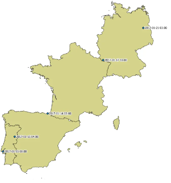
This information is also exported to be used on QGIS as a visual aid with a map of the visited countries and moments where the driver is on certain cities. In Figure 4.1 driver 1 with schedule 1 is departing from Lisbon on 2017-01-15 00:00, arriving at Guarda on 2017-01-15 04:00, reaching San Sebastian on 2017-01-16 03:00, passing through Saarbrucken on 2017-01-17 10:00, and arriving to the destination Berlin on 2017-01-21 03:00.
Figure 4.1: Example of the map from Lisbon to Berlin, with driver 1, schedule 1 information.
of every destination file. These files will have the costs per destination. One of these files (Table 4.3) will have the costs of worked hours and the other (Table 4.4) will have the costs per arriving moment in which the later one must be converted to tangible costs (Table 4.5). Then both of these files will be merged together with the importance of each file determined by the manager or the company. E.g.: the company determines that the costs of driven hours have 90% impact and the arriving time has only 10% of impact. This unbalance (later defined as alpha) is defined here when both files are combined, and it is completely up to the company or manager to decide. This information is needed to determine the best combination of drivers sent to fully satisfy the destinations’ needs.
Table 4.3: Example of the Complete Resume Matrix Hourly costs for 3 destinations. Driver type Schedule Madrid Paris Berlin
5 22 97.50 270.00 433.75 5 23 97.50 271.25 435.00 5 24 96.25 270.00 433.75 6 1 97.50 261.25 438.75 6 2 95.00 260.00 438.75 6 3 93.75 257.50 435.00 6 4 93.75 256.25 432.50 6 5 92.50 255.00 431.25 6 6 91.25 258.75 438.75 6 7 90.00 257.50 437.50 6 8 88.75 256.25 436.25 6 9 87.50 255.00 435.00 6 10 87.50 255.00 435.00 6 11 87.50 255.00 435.00 6 12 87.50 255.00 435.00 6 13 87.50 255.00 435.00 6 14 87.50 255.00 435.00 6 15 88.75 256.25 436.25 6 16 91.25 258.75 437.50 6 17 92.50 260.00 438.75 6 18 93.75 261.25 440.00 6 19 93.75 261.25 440.00 6 20 95.00 263.75 442.50 6 21 96.25 262.50 441.25 6 22 97.50 265.00 442.50 6 23 97.50 266.25 432.50 6 24 97.50 267.50 435.00 7 1 95.00 260.00 438.75 7 2 93.75 257.50 435.00 7 3 93.75 256.25 435.00 7 4 92.50 255.00 433.75 7 5 91.25 258.75 438.75
Table 4.4: Example of the Complete Resume Matrix Arriving moments for 3 destinations.
Driver type Schedule Madrid Paris Berlin
5 22 2017-01-18 06:00 2017-01-20 03:00 2017-01-24 08:00 5 23 2017-01-18 07:00 2017-01-20 03:00 2017-01-24 07:00 5 24 2017-01-18 08:00 2017-01-20 03:00 2017-01-24 07:00 6 1 2017-01-17 08:00 2017-01-19 03:00 2017-01-23 00:00 6 2 2017-01-17 09:00 2017-01-19 04:00 2017-01-23 01:00 6 3 2017-01-17 10:00 2017-01-19 04:00 2017-01-23 00:00 6 4 2017-01-17 11:00 2017-01-19 04:00 2017-01-22 23:00 6 5 2017-01-17 12:00 2017-01-19 04:00 2017-01-20 10:00 6 6 2017-01-17 13:00 2017-01-20 04:00 2017-01-23 08:00 6 7 2017-01-17 14:00 2017-01-20 04:00 2017-01-23 08:00 6 8 2017-01-17 15:00 2017-01-20 04:00 2017-01-23 08:00 6 9 2017-01-17 16:00 2017-01-20 04:00 2017-01-23 08:00 6 10 2017-01-17 17:00 2017-01-20 04:00 2017-01-23 08:00 6 11 2017-01-17 18:00 2017-01-20 04:00 2017-01-23 08:00 6 12 2017-01-17 19:00 2017-01-20 04:00 2017-01-23 08:00 6 13 2017-01-17 20:00 2017-01-20 04:00 2017-01-23 08:00 6 14 2017-01-17 21:00 2017-01-20 04:00 2017-01-23 08:00 6 15 2017-01-17 22:00 2017-01-20 04:00 2017-01-23 08:00 6 16 2017-01-17 23:00 2017-01-20 03:00 2017-01-23 07:00 6 17 2017-01-18 00:00 2017-01-20 03:00 2017-01-23 07:00 6 18 2017-01-18 01:00 2017-01-20 03:00 2017-01-23 07:00 6 19 2017-01-18 02:00 2017-01-20 03:00 2017-01-23 07:00 6 20 2017-01-18 03:00 2017-01-20 03:00 2017-01-23 06:00 6 21 2017-01-18 04:00 2017-01-20 03:00 2017-01-23 07:00 6 22 2017-01-18 05:00 2017-01-20 03:00 2017-01-23 05:00 6 23 2017-01-18 06:00 2017-01-20 03:00 2017-01-24 04:00 6 24 2017-01-18 07:00 2017-01-20 03:00 2017-01-24 03:00 7 1 2017-01-17 09:00 2017-01-19 04:00 2017-01-23 01:00 7 2 2017-01-17 10:00 2017-01-19 04:00 2017-01-23 00:00 7 3 2017-01-17 11:00 2017-01-19 04:00 2017-01-22 23:00 7 4 2017-01-17 12:00 2017-01-19 04:00 2017-01-20 10:00 7 5 2017-01-17 13:00 2017-01-20 04:00 2017-01-23 08:00
Table 4.5: Example of the Complete Resume Matrix Arriving moments adjusted to costs, for 3 destina-tions.
Driver type Schedule Madrid Paris Berlin
5 22 70 92 173 5 23 71 92 172 5 24 72 92 172 6 1 48 68 141 6 2 49 69 142 6 3 50 69 141 6 4 51 69 140 6 5 52 69 79 6 6 53 93 149 6 7 54 93 149 6 8 55 93 149 6 9 56 93 149 6 10 57 93 149 6 11 58 93 149 6 12 59 93 149 6 13 60 93 149 6 14 61 93 149 6 15 62 93 149 6 16 63 92 148 6 17 64 92 148 6 18 65 92 148 6 19 66 92 148 6 20 67 92 147 6 21 68 92 148 6 22 69 92 146 6 23 70 92 169 6 24 71 92 168 7 1 49 69 142 7 2 50 69 141 7 3 51 69 140 7 4 52 69 79 7 5 53 93 149
To finish, resorting to linear programming using an R package called ”Rglpk”, it will be determined what set of drivers will be traveling to what destination and on what schedule, minimizing the global costs.