Leonardo Bursztyn, Florian Ederer, Bruno Ferman and
Noam Yuchtman
Understanding mechanisms underlying
peer effects: evidence from a field
experiment on financial decisions
Article (Accepted version)
(Refereed)
Original citation:Bursztyn, Leonardo and Ederer, Florian and Ferman, Bruno and Yuchtman, Noam (2014) Understanding mechanisms underlying peer effects: evidence from a field experiment on financial decisions. Econometrica, 82 (4). pp. 1273-1301. ISSN 0012-9682
DOI: https://doi.org/10.3982/ECTA11991
© 2014 The Econometric Society
This version available at: http://eprints.lse.ac.uk/91509/
Available in LSE Research Online: January 2019
LSE has developed LSE Research Online so that users may access research output of the School. Copyright © and Moral Rights for the papers on this site are retained by the individual authors and/or other copyright owners. Users may download and/or print one copy of any article(s) in LSE Research Online to facilitate their private study or for non-commercial research. You may not engage in further distribution of the material or use it for any profit-making activities or any commercial gain. You may freely distribute the URL (http://eprints.lse.ac.uk) of the LSE Research Online website.
This document is the author’s final accepted version of the journal article. There may be differences between this version and the published version. You are advised to consult the publisher’s version if you wish to cite from it.
Understanding Mechanisms Underlying Peer Effects:
Evidence from a Field Experiment on Financial
Decisions
∗
Leonardo Bursztyn
†Florian Ederer
‡Bruno Ferman
§Noam Yuchtman
¶March 16, 2014
AbstractUsing a high-stakes field experiment conducted with a financial brokerage, we implement a novel design to separately identify two channels of social influence in financial decisions, both widely studied theoretically. When someone purchases an asset, his peers may also want to purchase it, both because they learn from his choice (“social learning”) and because his possession of the asset directly affects others’ utility of owning the same asset (“social utility”). We randomize whether one member of a peer pair who chose to purchase an asset has that choice implemented, thus randomizing his ability to possess the asset. Then, we randomize whether the second mem-ber of the pair: (1) receives no information about the first memmem-ber, or (2) is informed of the first member’s desire to purchase the asset and the result of the randomization that determined possession. This allows us to estimate the effects of learning plus possession, and learning alone, relative to a (no information) control group. We find that both social learning and social utility channels have statistically and economically significant effects on investment decisions. Evidence from a follow-up survey reveals that social learning effects are greatest when the first (second) investor is financially sophisticated (financially unsophisticated); investors report updating their beliefs about asset quality after learning about their peer’s revealed preference; and, they report motivations consistent with “keeping up with the Joneses” when learning about their peer’s possession of the asset. These results can help shed light on the mechanisms underlying herding behavior in financial markets and peer effects in consumption and investment decisions. JEL Codes: C93, D03, D14, D83, G02, M31
∗We would like to thank the co-editor and three anonymous referees, Sushil Bikhchandani, Aislinn Bohren, Arun
Chandrasekhar, Shawn Cole, Rui de Figueiredo, Fred Finan, Uri Gneezy, Dean Karlan, Navin Kartik, Larry Katz, Peter Koudijs, Kory Kroft, Nicola Lacetera, David Laibson, Edward Leamer, Phil Leslie, Annamaria Lusardi, Kristof Madarasz, Gustavo Manso, Ted Miguel, Kris Mitchener, Adair Morse, Paul Niehaus, Andrew Oswald, Yona Rubin-stein, Andrei Shleifer, Ivo Welch, as well as seminar participants at Berkeley, Columbia, FGV-SP, Frankfurt, GWU, HBS, LSE, MIT, Munich, NYU, PUC-Rio, UCLA, UCSD, SEEDEC, Simon Fraser, SITE, Stanford, Vienna, Yale, Yonsei and Zurich for helpful comments and suggestions. Juliana Portella provided excellent research assistance. We also thank the Garwood Center for Corporate Innovation, the Russell Sage Foundation and UCLA CIBER for financial support. Finally, we thank the management and staff of the cooperating brokerage firm for their efforts during the implementation of the study. There was no financial conflict of interest in the implementation of the study; no author was compensated by the partner brokerage or by any other entity for the production of this article.
†UCLA Anderson and NBER, [email protected]. ‡Yale School of Management, [email protected].
§Sao Paulo School of Economics - FGV, [email protected]. ¶UC-Berkeley Haas and NBER, [email protected].
1
Introduction
People’s choices often look like the choices made by those around them: we wear what is fashionable, we “have what they’re having,” and we try to “keep up with the Joneses.” Such peer effects have been analyzed across fields in economics.1 Motivated by concerns over herding and financial market
instability, an especially active area of research has examined the role of peers in financial decisions. Beyond studying whether peers affect financial decisions, different channels through which peer effects work have generated their own literatures linking peer effects to investment decisions, and to financial market instability. Models of herding and asset-price bubbles, potentially based on very little information, focus on learning from peers’ choices (Bikhchandani and Sharma, 2000; Chari and Kehoe, 2004). Models in which individuals’ relative income or consumption concerns drive their choice of asset holdings, and artificially drive up some assets’ prices, focus on peers’
possession of an asset.2 In this paper, we use a high-stakes field experiment, conducted with a
financial brokerage, to separately identify the causal effects of these channels through which a person’s financial decisions are affected by his peers’.
Identifying the causal effect of one’s peers’ behavior on one’s own is notoriously difficult (see, for example, Manski, 1993). Equally difficult is identifying why one’s consumption or investment choices have a social component. Broadly, there are two reasons why a peer’s act of purchasing an asset (or product, more generally) would affect one’s own choice. First, one may infer that assets (or products) purchased by others are of higher quality; we refer to this as social learning. Second, one’s utility from possessing an asset (or product) may depend directly on the possession of that asset (or product) by another individual; we call this social utility.
Suppose an investor i considers purchasing a financial asset under uncertainty. In canonical models of herding based on social learning, information that a peer, investor j, purchased the asset will provide favorable information about the asset to investor i: investor j (acting in isolation) would only have purchased the asset if he observed a relatively good signal of the asset’s return. The favorable information conveyed by investor j’s revealed preference increases the probability that investor i purchases the asset, relative to making a purchase decision in isolation.3
A direct effect of investor j’s possession of a financial asset on investor i’s utility might arise for
1Seminal theoretical articles include Banerjee (1992) and Bikhchandani et al. (1992). Early empirical research
includes Case and Katz (1991), Katz et al. (2001), Sacerdote (2001), and Zimmerman (2003). Durlauf (2004) surveys the literature on neighborhood effects. Peer effects have also been studied by psychologists and sociologists: influential social psychology research includes Asch (1951) and Festinger (1954); a review of empirical research on peer effects in sociology is presented in Jencks and Mayer (1990).
2Preferences over relative consumption can arise from the (exogenous) presence of other individuals’ consumption
decisions in one’s utility function, (e.g. Abel, 1990, Gali, 1994, Campbell and Cochrane, 1999) or can arise endoge-nously when one consumes scarce consumption goods, the prices of which depend on the incomes (and consumption and investment decisions) of other individuals (DeMarzo et al., 2004, DeMarzo et al., 2008). For an overview, see Hirshleifer and Teoh (2003).
3Avery and Zemsky (1998) present a model in which prices adjust in response to herding behavior; however, in
a variety of reasons widely discussed in the finance literature. First, investors may be concerned with their incomes or consumption levels, relative to their peers’ (“keeping up with the Joneses”, as in Abel, 1990, Gali, 1994, and Campbell and Cochrane, 1999).4 Second, investor j’s possession
of a financial asset may affect investor i’s utility through “joint consumption” of the asset: peers can follow and discuss financial news together, track returns together, etc. (Taylor, 2011, describes the popularity of “investment clubs” in the 1990s). The impact of a peer’s possession of an asset on an individual’s utility derived from owning the same asset (for multiple reasons) is the social utility channel.5
Typically, investor j’s decision to purchase the asset will also imply that investor j possesses the asset. Thus, a comparison of investor i’s investment when no peer effect is present to the case in which he observes investor j purchasing an asset will generally identify the combined social learning and social utility channels. To disentangle social learning from social utility, one needs to identify, or create, a context in which investor j’s decision to purchase an asset is decoupled from investor j’s possession of the asset.6
Our experimental design (discussed in detail in Section 2) represents an attempt to surmount both the challenge of identifying a causal peer effect, and the challenge of separately identifying the effects of social learning and social utility. Working closely with us, a large financial brokerage in Brazil offered a new financial asset to pairs of clients who share a social relationship. The stakes were high: minimum investments were R$2,000 (over $1,000 U.S. dollars at the time of the study), around 50% of the median investor’s monthly income in our sample.
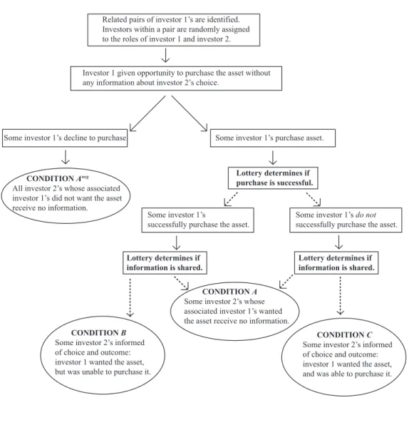
To identify any sort of peer effect on investment decisions, we randomly informed one member of the peer pair, investor 2, of the investment made by the other member of the pair, investor 1 (assignment to the roles of investor 1 and investor 2 was random). To disentangle the effect of investor 1’s possession from the effect of the information conveyed by investor 1’s revealed preference, we exploit a novel aspect of our experimental design. The financial brokerage with which we worked implemented a lottery to determine whether individuals who chose to purchase the asset would actually be allowed to make the investment (see Figure 1 for a graphical depiction of the experimental design). Thus, half of the investor 1’s who chose to purchase the asset revealed a preference for the financial asset, but did not possess it.
Among investor 1’s who chose to purchase the asset, we implemented a second, independent randomization to determine the information received by the associated investor 2’s: we randomly
4Evidence consistent with individuals caring about relative outcomes has been presented by Luttmer (2005),
Fliessbach et al. (2007), and Card et al. (2010), among others.
5Note that even in the absence of truly “social” preferences, one might observe greater demand for an asset simply
because a peer holds it: for example, this might arise as a result of competition over scarce consumption goods. Because we do not wish to abuse the term, “social preferences,” we prefer the broader term, “social utility.” Note also that social utility might lead to negative correlations between peers’ choices (see Clark and Oswald, 1998); for example, one might observe a demand for joint insurance (see, e.g., Angelucci et al., 2012).
6In Appendix B (all appendices are online) we present a model of peer effects in financial decisions that features
assigned investor 2 to receive either no information about investor 1’s investment decision, or to receive information about both the investment decision and the outcome of the lottery determining possession. Thus, among investor 1’s who chose to purchase the asset, the associated investor 2’s were randomly assigned to one of three conditions: in condition A, no information about investor 1’s decision was provided; in condition B, investor 2’s received information that investor 1 made a decision to purchase the asset, but was not able to consummate the purchase (so learning occurred
without possession); and, in condition C, investor 2’s received information that investor 1 made a
decision to purchase the asset, and was able to consummate the purchase (so learning occurred, along with possession). A comparison of choices made by investor 2’s in conditions A and B reveals the effect of social learning; a comparison of conditions B and C reveals the impact of investor 1’s possession of the asset over and above the information conveyed by his purchase, that is, social utility; a comparison of conditions A and C reveals the total effect of these two channels.
Our experimental evidence suggests that both channels through which peer effects work are economically and statistically significant. Among investor 2’s whose peer chose to purchase the asset we find the following: in the “no information” condition A, 42% chose to purchase the asset; in the “social learning only” condition B, the take-up rate increased to 71%; finally, in the “social learning plus social utility” condition C, the rate increased to 93%. Not only do individuals learn from their peers, but there is also an effect of possession beyond learning.
To better understand investors’ decision making in the different conditions, and to help us evaluate alternative interpretations of the treatment effects we observe, we partnered with the brokerage to conduct a follow-up survey of the investors in the study (see Section 2.4 for details). We first analyze the social learning channel, presenting evidence of positive belief updating among investor 2’s who learned about their peers’ purchase decisions, and of heterogeneous social learning effects consistent with a model in which unsophisticated investors learn more from others’ purchases, and sophisticated investors’ purchases are more influential. We also find evidence suggestive of social utility concerns among investors who chose to purchase the asset in condition C. The evidence from the follow-up survey additionally helps us rule out several alternative interpretations of the treatment effects we observe, as well as confounding factors (we discuss alternative hypotheses and limitations of our study further in Section 3).
Our work contributes most directly to the empirical literature on peer effects in investment decisions, some observational (e.g., Hong et al., 2004, Hong et al., 2005, Ivkovic and Weisbenner, 2007, Brown et al., 2008, Li, 2009, and Banerjee et al., 2011), some experimental (e.g., Duflo and Saez, 2003, Beshears et al., 2011). Our paper goes beyond the existing literature by using experimental variation to separately identify the causal roles of different channels of peer effects. Disentangling these channels is of more than academic interest: it can provide important, policy-relevant evidence on the sources of herding behavior in financial markets. Our findings of significant social learning and social utility effects suggest that greater information provision might mitigate
– but not eliminate – herding behavior.
Our paper also contributes to the broader empirical literature on social learning and peer effects.7 As in our work, several recent papers use information shocks to identify causal peer effects
(e.g., Frey and Meier, 2004, Chen et al., 2010, Ayres et al., 2009, Costa and Kahn, 2010, and Allcott, 2011). However, the information shocks they exploit do not allow for the separate identification of the channels through which peer effects work. Identifying the effect of social learning alone is the focus of Cai et al. (2009) and Moretti (2011); they try to rule out the existence of peer effects through other channels (e.g., joint consumption), but they do not experimentally manipulate the social utility channel. Cai et al. (2012) use experimental variation in the field to identify the effects of different types of social learning; Maertens (2012) uses non-experimental methods to study different channels of social influence; Cooper and Rege (2011) attempt to distinguish among peer effect channels in the lab. Our work is the first we know of that uses experimental variation in the field to isolate the effect of social learning and the separate effect of social utility. Our results corroborate models of social learning such as Banerjee (1992) and Bikhchandani et al. (1992), but indicate that peers’ purchasing decisions have effects beyond social learning as well.
Finally, our experimental design, which allows us to separately identify the channels through which peer effects work, represents a methodological contribution. As we discuss in the conclusion, our design could be applied toward the understanding of social influence in marketing, technology adoption, and health-promoting behavior.
The paper proceeds as follows: in Section 2, we describe in detail our experimental design, which attempts to separately identify the channels through which peer effects work; in Section 3, we present our empirical specification and the results of our experiment, and discuss our findings; finally, in Section 4, we offer concluding thoughts.
2
Experimental Design
The primary goal of our design was to decouple a peer’s decision to purchase the asset from his possession of the asset. We generated experimental conditions in which individuals would make decisions: 1) uninformed about any choices made by their peer; 2) informed of their peer’s revealed preference to purchase an asset, but the (randomly determined) inability of the peer to make the investment; and, 3) informed of their peer’s revealed preference to purchase an asset, and the peer’s (randomly determined) successful investment.
7Empirical work on peer effects has studied a wide range of outcomes, for example, education, compensation, and
charitable giving (Sacerdote, 2001; Carrell and Hoekstra, 2010; de Giorgi et al., 2010; Duflo et al., 2011; Card and Giuliano, 2011; Shue, 2012; DellaVigna et al., 2012); the impact of one’s peers and community on social indicators and consumption (Bertrand et al., 2000; Kling et al., 2007; Bobonis and Finan, 2009; Dahl et al., 2012; Grinblatt et al., 2008; Kuhn et al., 2011); and, the impact of coworkers on workplace performance (Guryan et al., 2009; Mas and Moretti, 2009; Bandiera et al., 2010). Herding behavior and informational cascades (Celen and Kariv, 2004) and the impact of cultural primes on behavior (Benjamin et al., 2010) have been studied in the lab.
2.1
Designing the Asset
The asset being offered needed to satisfy several requirements. Most fundamentally, there needed to be a possibility of learning from one’s peers’ decisions. In addition, because many of our comparisons of interest are among investor 2’s whose associated investor 1’s chose to purchase the asset, the asset needed to be sufficiently desirable that enough investor 1’s would choose to purchase it. To satisfy these requirements, the brokerage created a new, risky asset specifically for this study. The asset is a combination of an actively-managed, open-ended long/short mutual fund and a real estate note (Letra de Cr´edito Imobili´ario, or LCI) for a term of one year. The long/short fund seeks to
outperform the interbank deposit rate (CDI, Certificado de Dep´osito Interbanc´ario) by allocating
investment funds to fixed-income assets, equity securities, and derivatives. The LCI is a low-risk asset that is attractive to personal investors because it is exempt from personal income tax; it can be thought of as an appealing, high-yield CD.
The LCI offered in this particular combination had somewhat better terms than the real estate notes that were usually offered to clients of the brokerage, thus generating sufficient demand to meet the experiment’s needs. First, the return of the LCI offered in the experiment was 98% of the CDI, while the best LCI offered to clients outside of the experiment had a return of 97% of the CDI. In addition, the brokerage firm usually required a minimum investment of R$10,000 to invest in an LCI, while the offer in the experiment reduced the minimum investment threshold to R$1,000 (the long/short fund also required a minimum investment of R$1,000). The brokerage piloted the sale of the asset (without using a lottery to determine possession), to clients other than those in the current study, in order to ensure a purchase rate of around 50%.
Another requirement was that there be no secondary market for the asset, for several reasons. First, we hoped to identify the impact of learning from peers’ decisions to purchase the asset, rather than learning from peers based on their experience possessing the asset. Investor 2 may have chosen not to purchase the asset immediately, in order to talk with investor 1, then purchase the asset from another investor. We wished to rule out this possibility. In addition, we did not want peer pairs to jointly make decisions about selling the asset. Finally, we did not want investor 2 to purchase the asset in hopes of selling it to investor 1 when investor 1’s investment choice was not implemented by the lottery. In response to these concerns, the brokerage offered the asset only at the time of their initial phone call to the client and structured the asset as having a fixed term with no resale. A final requirement, given our desire to decouple the purchase decision from possession, was that there must be limited entry into the fund to justify the lottery to implement purchase decisions. The brokerage was willing to implement the lottery design required, justified by the supply constraint for the asset they created. At the individual level, the maximum investment in the LCI component was set at R$10,000.
2.2
Selling the Asset
To implement the study, we designed (in consultation with the financial brokerage) a script for sales calls that incorporated the randomization necessary for our experimental design (the translated script is available in Appendix C).8 The brokerage required that calls be as natural as possible: sales calls had frequently been made by the brokerage in the past, and our script was made as similar as possible to these more typical calls. In addition, the experimental calls were made by the individual brokers who were accustomed to working with the clients they called as part of the study. Thus, we (and the brokerage) expected that clients would trust the broker’s claims about their peer’s choices, and to believe that the lottery would be implemented as promised.
Between January 26, and April 3, 2012, brokers called 150 pairs of clients whom the brokerage had previously identified as having a social connection (48% are members of the same family, and 52% are friends; see Appendix Table A.1).9 Information on these clients’ social relationships was
available for reasons independent of the experiment: the firm had made note of referrals made by clients in the past. This is particularly important because clients’ social relationships would not have been salient to those whose sales call did not include any mention of their peer. We thus believe that without any mention of the offer being made to the other member of the peer pair, there should be practically no peer effect.10
One member of the pair was randomly assigned to the role of “investor 1,” and the other assigned to the role of “investor 2.”11 Investor 1 was called by the brokerage and given the opportunity to
invest in the asset without any mention of their peer. The calls proceeded as follows. The asset was first described in detail to investor 1. After describing the investment strategy underlying the asset, the investor was told that the asset was in limited supply; in order to be fair to the brokerage’s clients, any purchase decision would be confirmed or rejected by computerized lottery (this is not as unusual as it may appear; for example, Instefjord et al. (2007) describe the use of lotteries to allocate shares when IPO’s are oversubscribed). If the investor chose to purchase the asset, he was asked to specify a purchase amount (investors were not allowed to convert existing
8We created the script using Qualtrics, a web-based survey platform. Occasionally, Qualtrics was abandoned
when the website was not accessible, and the brokers used Excel to generate the randomization needed to execute the experimental design. Treatment effects are very similar if we restrict ourselves to the Qualtrics calls (results available upon request).
9The sample size was limited by the number of previously-identified socially-related pairs of clients, as well the
brokerage’s willingness to commit time to the experiment. The brokerage agreed (in advance of the calls) to reach 300 clients. A photo of the brokerage making sales calls as part of the experiment (with our research assistant present) is included in Appendix C.
10We also asked the brokerage if any investor spontaneously mentioned their peer in the sales call, and the brokerage
indicated that this never occurred. If an individual in condition A had thought about his peer’s potential offer and purchase of the same asset, our measured peer effects would be attenuated.
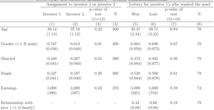
11A comparison of the characteristics of investor 1’s and investor 2’s can be seen in Appendix Table A.2, columns
1 and 2. The randomization resulted in a reasonable degree of balance across groups: 4 of 5 tests of equality of mean characteristics across groups have p-values above 0.10. One characteristic, gender, is significantly different across groups.
investments with the brokerage, and thus allocated new resources in order to purchase the asset). Then, a computer would generate a random number from 1 to 100 (during the phone call), and if the number was greater than 50, the investment would be authorized.12
Following the call to investor 1, the same broker called the associated investor 2. The brokers were told that, for each pair, both investors had to be contacted on the same day to avoid any communication about the asset that might contaminate the experimental design. Only 6 out of 150 investor 2’s had communicated with their associated investor 1’s about the asset prior to the phone call from the brokerage (dropping these 6 observations does not affect any of our results). If the broker did not succeed in reaching investor 2 on the same day as the associated investor 1, the broker would not attempt to contact him again; this outcome occurred for 12 investor 1’s, who are not included in our empirical analysis. Thus, brokers called 162 investor 1’s in order to attain our sample size of 150 pairs successfully reached.
When the broker reached investor 2, he began the script just as he did for investor 1: describing the asset, including the lottery to determine whether a purchase decision would be implemented. Next, during the call, the broker implemented the experimental randomization and attempted to sell the asset under the experimentally-prescribed conditions (described next). If investor 2 chose to purchase the asset, a random number was generated to determine whether the purchase decision would be implemented, just as was the case for investor 1.
2.3
Randomization into Experimental Conditions
The experimental conditions were determined as follows. Among the group of investor 1’s who chose to purchase the asset, their associated investor 2’s were randomly assigned to receive information about investor 1’s choice and the lottery outcome, or to receive no information. There was thus a “double randomization” – first, the lottery determining whether investor 1 was able to make the investment, and second, the randomization determining whether investor 2 would be informed about investor 1’s investment choice and the outcome of the first lottery.
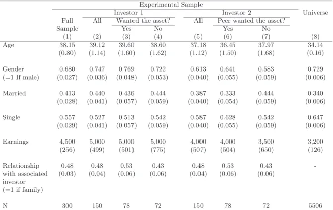
This process assigns investor 2’s whose associated investor 1’s chose to purchase the asset into one of three conditions (refer to Figure 1); investor characteristics across the three experimental conditions can be seen in Table 1 (we generally present means of the various investor characteristics, with the exception of the earnings variable, the median of which is shown in order to mitigate the influence of outliers). One-third were assigned to the “no information,” control, condition A. Half of these come from the pool of investor 2’s paired with investor 1’s who wanted the asset but were not authorized to make the investment, and half from those paired with investor 1’s who wanted
12Among investor 1’s who wanted to purchase the asset, a comparison of the characteristics of investor 1’s whose
purchase decision was authorized and investor 1’s whose purchase decision was not authorized can be seen in Appendix Table A.2. The randomization resulted in a reasonable degree of balance across groups: 5 of 6 tests of equality of mean characteristics across groups have p-values above 0.10. One characteristic, gender, is significantly different across groups.
to make the investment and were authorized to make it. Investor 2’s in condition A were offered the asset just as was investor 1, with no mention of an offer made to their peer.
Two-thirds received information about their peer’s decision to purchase the asset (but not the magnitude of the desired investment), as well as the outcome of the lottery that determined whether the peer was allowed to invest. The randomization resulted in approximately one-third of investor 2’s in condition B, in which they were told that their peer purchased the asset, but had that choice rejected by the lottery. The final third of investor 2’s were in condition C, in which they were told that their peer purchased the asset, and had that choice implemented by the lottery.
The three conditions of investor 2’s whose associated investor 1’s wanted to purchase the asset are the focus of our analysis. Given the double randomization in our experimental design, investor 2’s in conditions A, B, and C should have similar observable characteristics, and should differ only in the information they received. As a check of the randomization, we present in Table 1 the individual investors’ characteristics for each of the three groups, as well as tests of equality of the characteristics across groups. As expected from the random assignment, the sample is well balanced across the baseline variables.
Along with the three conditions of interest, in some analyses we will consider those investor 2’s whose associated investor 1 chose not to invest in the asset (the characteristics of these investor 2’s can be seen in Appendix Table A.1, column 7). We assign these investor 2’s to their own “negative selection” condition Aneg, in which they receive no information about their peer. We did not reveal
their peers’ choices because the brokerage did not want to include experimental conditions in which individuals learned that their peer did not want the asset. These individuals were offered the asset in exactly the same manner as were investor 1’s and investor 2’s in condition A. We refer to this condition as “negative selection,” because the investor 2’s in condition Aneg are those whose peers
specifically chose not to purchase the asset.
Our experimental design allows us to estimate overall peer effects, and to disentangle the chan-nels through which peers’ purchases affect investment decisions. A comparison of those in conditions
A and C reveals the standard peer effect. A comparison of investors in conditions A and B allows
us to estimate the impact of social learning resulting from a peer’s decision but without
posses-sion. Comparing investor 2’s in conditions B and C will then allow us to estimate the impact of a
peer’s possession alone, over and above learning from a peer’s decision.13 In addition to identifying these peer effects, we will examine the role of selection into peer pairs according to preferences, by comparing investor 2’s in condition A to those in the condition Aneg.
13It is important to emphasize that our estimated effect of possession is conditional on investor 2 having learned
about the asset from the revealed preference of investor 1 to purchase the asset. One might imagine that the effect of possession of the asset by investor 1 without any revealed preference to purchase the asset could be different. It is also important to point out that the estimated effect of “possession” is difficult to interpret quantitatively: the measured effect is bounded above by 1 minus the take-up in condition B, working against finding any statistically significant peer effects beyond social learning.
2.4
Follow-up Survey
Between November 26, and December 7, 2012, the brokerage conducted a follow-up survey with a subset of the clients from the main study; investors were told (truthfully) that the brokerage wished to learn about its clients in order to provide them with more individualized services and information. The follow-up survey was conducted with two primary goals for the purposes of our work: first, to measure investors’ financial sophistication; and second, to collect information that could be used to better understand the decision making processes behind the choices of investor 2’s (for the English language survey questionnaires, see Appendix C).
In our analysis below, we examine heterogeneity in social learning effects among investor 2’s in conditions A and B, depending on whether investor 2, or the associated investor 1, is financially sophisticated. To measure the relevant set of investors’ financial sophistication, the brokerage contacted the investor 2’s in conditions A and B, as well as their associated investor 1’s, and asked them to assess their own financial knowledge; in addition, the brokerage asked these investors a series of objective questions measuring financial literacy.14 For summary statistics on the financial
sophistication survey questions, see Appendix Table A.3, Panel A.
We also collected survey evidence that can help us understand the decision making of investor 2’s across experimental conditions A, B, and C. In particular, we asked about several aspects of investors’ decisions: (i) how investors viewed the lottery that determined whether purchase decisions were implemented (surveying investors in conditions A, B, and C ); (ii) how investors responded to information about their peer’s purchase decision and lottery result, as well as whether the information provided by brokers was credible (surveying investors in conditions B and C ); (iii) whether investors’ decisions were specifically affected by their peer’s lost lottery (condition B ); and, (iv) whether social utility considerations affected investors’ decisions to purchase the asset (investors in condition C who chose to purchase the asset). For summary statistics on the decision making survey questions, see Appendix Table A.3, Panel B.
It is important to highlight two weaknesses of the follow-up survey. First, investors may have responded in ways that they thought would please the surveyor. It is important to note, however, that the vast majority (over 90%) of survey calls were not made by the investor’s usual broker, but by another broker at the firm, with whom investors did not have a personal relationship. This mitigates concerns about surveyor demand effects (results are very similar excluding surveys in which the survey was conducted by the broker who made the experimental sales call, see Appendix Table A.4). In addition, many of the questions asked, such as those regarding financial sophisti-cation or the updating of beliefs, did not have an answer that would be viewed more favorably by
14The specific questions come from the National Financial Capability Survey (translated into Portuguese), and
have been used in studies both in the US and in other countries (Lusardi and Mitchell, 2011a,b). Investor 2’s other than those in conditions A and B, and investor 1’s other than those associated with investor 2’s in conditions A and B, were not asked these financial sophistication questions to reduce the brokerage’s time commitment to the follow-up survey.
the brokerage. Second, the questions aimed at understanding investors’ decision making were not open-ended, but were directed toward the mechanisms of interest. This was necessary in order to limit the time committed by the brokerage (and investors) to the follow-up survey, and to reduce the amount of noise present in the survey responses. These weaknesses should be kept in mind when interpreting the follow-up survey evidence.
The brokerage conducted the follow-up survey over the phone, calling investor 2’s in conditions
A, B, and C, and investor 1’s associated with investor 2’s in conditions A and B, up to three times
each; the brokerage was able to reach 90.4% of the investors called.
3
Empirical Analysis
3.1
Regression Specification
To identify the experimental treatment effects, we estimate regression models of the following form:
Yi= α +
X
c
βcIc,i+ γ′Xi+ ǫi. (1)
Yi is an investment decision made by investor i: in much of our analysis it is a dummy variable
indicating whether investor i wanted to purchase the asset, but we also consider the quantity invested, as well as an indicator that the investment amount was greater than the minimum required. The variables Ic,iare indicators for investor i being in category c, where c indicates the experimental
condition to which investor i was assigned. In all of our regressions, the omitted category of investors to which the others are compared is investor 2’s in condition A: investor 2’s associated with a peer who wanted to purchase the asset, but who received no information about their peer. In much of our analysis, we focus on investor 2’s, so c ∈ {condition B , condition C , condition Aneg}. In
some cases, we include investor 1’s in our analysis, and they will be assigned their own category c. Finally, in some specifications we include control variables: Xi is a vector that includes broker
fixed effects and investor characteristics.
3.2
Empirical Estimates of Peer Effect Channels
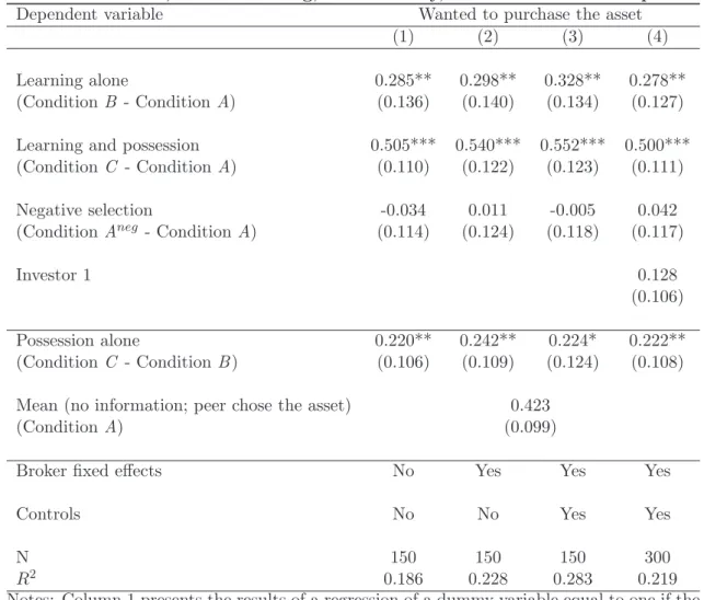
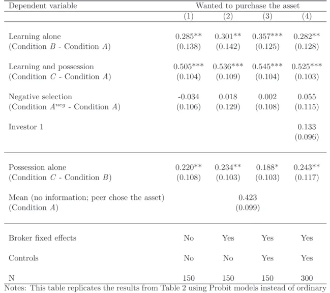
We first present the treatment effects of interest using an indicator of the investor’s purchase decision as the outcome variable, and various specifications estimated using OLS, in Table 2 (results are very similar using probit or logit models; see Appendix Tables A.5 and A.6). We begin by estimating a model using only investor 2’s and not including any controls, in Table 2, column 1. These results are equivalent to comparing means in the raw data (which are presented in Appendix Figure A.1). Treatment effects are estimated relative to the omitted category, investor 2’s in condition
A, who had a take-up rate of 42%. In the “social learning alone” condition B, the take-up rate
“social learning plus social utility” condition C, the take-up rate was 93%, significantly larger than the take-up rate in both conditions A and B.15 These differences represent economically and
statistically significant overall peer effects and indicate that social learning without possession affects the investment decision, as does possession beyond social learning. Finally, the coefficient on the indicator for condition Aneg is economically small, and it is not statistically significant, suggesting
that “selection” effects are small in our setting.
A natural question about Table 2 is whether our statistical inferences are sound, given the rela-tively small number of observations in each experimental condition. As an alternative to standard t-tests to determine statistical significance, we ran permutation tests with 10,000 repetitions for pairwise comparisons of take-up rates across conditions A, B, C, and Aneg. To run the permutation
tests, we randomly assign “placebo treatment” status to investors in the conditions of interest, 10,000 times, and calculate a distribution of “placebo treatment effects.” We then compare the size of the treatment effects we find using the actual treatment assignment to the distribution of “placebo treatment effects.” While the permutation test is not an exact test, it can complement our inferences using t-tests. For our main comparisons, we find p-values that are trivially larger using permutation tests than using t-tests, but our inferences are unchanged, suggesting that inferences using t-tests are valid (see Appendix Table A.8, Panel A, column 1).
We next present regression results including broker fixed effects (Table 2, column 2) and in-cluding both broker fixed effects and baseline covariates (column 3); then, we estimate a regression including these controls and using the combined sample of investor 1’s and investor 2’s in order to have more precision (column 4). The overall peer effect, as well as the individual social learn-ing and social utility channels, estimated uslearn-ing these alternative models are very similar across specifications (consistent with successful randomization across conditions).16
We now delve more deeply into our data, and analyze investors’ responses to the follow-up survey, in order to better understand the treatment effects we observe. We first present additional evidence on each of the two channels of social influence we study. Then, we discuss potential concerns with our experimental design and the interpretation of our results.
15The p-value from a test of equality between take-up rates in conditions A and C – the overall peer effect – is 0.000.
The p-value from a test that condition B equals condition A – social learning alone – is 0.043. The p-value from a test that condition C equals condition B – possession’s effect above social learning – is 0.044. Note that one might wish to compare take-up rates in conditions B and C to a broader “no information” control group than condition A. We use data on investors 1’s to estimate the take-up rate of positively-selected individuals using GMM, imposing the overidentifying restriction that investor 1’s take-up rate is a weighted average of investor 2’s in conditions A and Aneg. While social learning effects are smaller, our results are qualitatively unchanged (see Appendix Table A.7).
We prefer using individuals in condition A as the control group as it is most internally valid: investor 1’s calls came earlier in the day than calls to investor 2’s, and did not include the information randomization that was part of the calls made to the latter (a test of the overidentifying restriction in the GMM model also nearly rejects the null).
16Examining alternative outcomes – the amount investors chose to invest in the asset, or a dummy variable
in-dicating whether the investment amount was greater than the minimum required – yields very similar results (see Appendix Figure A.2 and Table A.9; for p-values calculated using permutation tests, see Table A.8, Panel A, columns 2–3).
3.3
Understanding the Social Learning Treatment Effects
Heterogeneity of social learning effects by financial sophistication. When observing a peer’s purchase of an asset, an investor with greater financial sophistication (and therefore a more precise signal of asset quality) should put less weight on information derived from their peer’s revealed preference, relative his own signal of the quality of the asset. Similarly, the information conveyed by the revealed preference of one’s peer should be more influential if this peer is more financially sophisticated, and is thus likely to have received a more precise signal of the asset’s quality (see Appendix B for a formal treatment of these arguments). We thus expect that the social learning channel should be more important for less financially sophisticated investor 2’s, and when investor 1’s were more financially sophisticated.
It is important to keep in mind that financial sophistication is not randomly assigned in our study, so it might be correlated with some other, unobserved characteristic. In addition, testing for heterogeneous treatment effects divides our sample into small cells; thus, evidence of heterogeneous treatment effects should be interpreted cautiously. Small cell sizes also prevent us from combining into a single analysis the study of social learning by sophisticated and unsophisticated investors with the study of social learning from sophisticated and unsophisticated investors. Still, exploring heterogeneous treatment effects is both interesting from a theoretical standpoint – since it is a natural extension of a social learning framework – and it can also provide suggestive evidence that our measured social learning treatment effects are not driven by other factors.
We construct two measures of investors’ financial sophistication using responses to several ques-tions included in our follow-up survey (for the English version of the questionnaire used in the survey, see Appendix C; for summary statistics on the financial sophistication survey questions, see Appendix Table A.3, Panel A). Our first measure captures investors’ self-assessments of their financial sophistication, on a 1 to 7 scale. We define “financially sophisticated” investors as those who reported a number greater than or equal to 4, producing the most even split of our sample. Our second measure captures investors’ objective financial knowledge, based on four questions testing respondents’ understanding of important concepts for investing: compounding; inflation; diversifi-cation; and, the relationship between bond prices and interest rates. The objective measure defines “financially sophisticated” investors as those who correctly answered 3 or more questions, again producing the most even split of our sample. Our two measures of financial sophistication have a correlation of around 0.4 within-investor; across peers in each pair, the correlation is just 0.06 for the self-assessed measure, and -0.11 for the objective measure. For brevity, in the text we will present tests of heterogeneity in social learning across both investor 1’s and investor 2’s levels of financial sophistication using only the self-assessed measure (in Appendix Table A.10, we present the same specifications shown in the text, but using the objective measure, and our results are very similar).
2’s in conditions A and B ), with the take-up rate as the outcome variable, for different categories of investor 2’s. In Table 3, Panel A, we present social learning treatment effects estimated from regressions without controls (i.e., comparisons of means). In columns 1–2, we estimate separate social learning effects for financially sophisticated and financially unsophisticated investor 2’s, re-spectively. We regress the investment decision dummy variable on a “financially sophisticated” indicator; an interaction between a condition B indicator and the financially sophisticated indi-cator; and, an interaction between a condition B indicator and a “financially unsophisticated” indicator. In columns 4–5, we estimate separate social learning effects for investor 2’s associated with financially sophisticated and financially unsophisticated investor 1’s, respectively. We esti-mate regressions analogous to columns 1–2, but substitute indicators of the associated investor 1’s financial sophistication for the indicators of investor 2’s financial sophistication. Panel B presents estimated social learning effects from models that include baseline controls and broker fixed effects. The results in Table 3 match our predictions. First, in columns 1–2, we observe small, sta-tistically insignificant social learning effects on financially sophisticated investor 2’s, and large, significant effects on unsophisticated investor 2’s.17 Column 3 shows that the difference between the treatment effects for sophisticated and unsophisticated investor 2’s is also statistically signif-icant. Next, in columns 4–5, we find large, statistically significant social learning effects among investor 2’s associated with financially sophisticated investor 1’s, and small, insignificant effects among investor 2’s associated with financially unsophisticated investor 1’s (take-up rates across sub-groups are presented in Appendix Figures A.3.1 and A.3.2). We find results that are very similar using the objective measure of financial knowledge (see Appendix Table A.10) or using alternative outcomes (amount invested or an indicator of an investment larger than the minimum; see Appendix Tables A.11 and A.12). To address concerns about statistical inferences given the small cell sizes, we ran permutation tests with 10,000 repetitions for each subgroup’s social learning effect, and our inferences are unaffected (p-values presented in Appendix Table A.8, Panel B).
Evidence of updated beliefs. We believe that investor 2’s higher take-up rate in condition
B, and a component of their higher take-up rate in condition C, resulted from positively updating
their beliefs about the asset after hearing that their associated investor 1 chose to purchase it. While brokers did not elicit prior or posterior beliefs during the initial sales call, in the follow-up survey, investors in conditions B and C were directly asked whether the fact that their associated investor 1 wanted to purchase the asset affected their beliefs about the quality of the asset. We find that 67% of investor 2’s in conditions B and C reported positively updating their beliefs about the quality of the asset after learning that their peer chose to purchase it, consistent with a social
17Unsophisticated investor 2’s have a lower take-up rate in condition A than do sophisticated investor 2’s. This
may be a result of sampling variation (the difference in take-up rates is not statistically significant) or a result of different prior beliefs about the asset in the absence of any peer effect. It is important to note that even if take-up rates in condition A were switched across groups, we would continue to find significant social learning effects among unsophisticated investor 2’s and no significant social learning effects among sophisticated investor 2’s.
learning effect; and, individuals who positively updated their beliefs were statistically significantly more likely to purchase the asset (the difference in take-up rates is 31 percentage points).
Our hypotheses regarding heterogeneous social learning effects according to investor 1’s and in-vestor 2’s financial sophistication suggest that unsophisticated inin-vestor 2’s should have been more likely to positively update their beliefs; and, purchase decisions by sophisticated investor 1’s should have led to more positive belief updating. Indeed, we find these patterns in the follow-up sur-vey data. Among unsophisticated investor 2’s in condition B, 92% reported positively updating their beliefs about the quality of the asset; among sophisticated ones, only 11% did (the p-value of this difference is less than 0.01). Among investor 2’s in condition B associated with sophisti-cated investor 1’s, we find that 69% positively updated their beliefs; among those associated with unsophisticated investor 1’s, only 33% updated positively (the p-value of this difference is 0.16).
3.4
Understanding the Social Utility Treatment Effects
The finance literature has pointed to different reasons why one’s peer’s possession of an asset might directly affect one’s utility from possessing the same asset. In the follow-up survey, the investor 2’s in condition C who chose to purchase the asset were asked about two particular mechanisms. First, they were asked about the importance of relative income or consumption concerns: whether earning the same return as their peer was important to their decision; whether fear of missing out on a return their peer might earn was important; and, whether they thought about what their peer might do with the returns from the asset. Second, they were asked one question relating to the importance of the “joint consumption” value of the financial asset: whether anticipated discussions of the asset with their peer were important to their decision.
The results indicate that both mechanisms were important. First, regarding “keeping up with the Joneses” motives: 60% of respondents reported that wanting to earn the same financial return as their peer was a significant factor in their decision; 80% of them reported that they thought about what their peer could do with the return from the asset; 32% reported that the fear of not having a return that their peer could have was a significant factor in their decision. We also find evidence of a “joint consumption” channel: 44% reported that a significant factor in their purchase decision was that they could talk with their peer about the asset. Although we cannot cleanly identify the relative importance of these different mechanisms, the evidence from the follow-up survey suggests that relative income and consumption concerns and a desire for “joint consumption” both played a role in generating the social utility effects we observe. Only 4% of respondents did not point to any of these social utility factors as a relevant element in their decision making process.
3.5
Alternative Hypotheses and Confounding Factors
In an ideal experiment, condition B would have differed from condition A only because of social learning; and, condition C would have differed from condition B only in the added effect of social utility. In practice, there may have been other differences across conditions; here we discuss whether they were likely to have played an important role in generating the treatment effects we find.
Effects of the lottery to authorize investments. One might wonder if the presence of the lottery distorted decisions by making the asset appear to be scarce and desirable. We do not believe this was the case. First, the asset used in the study could not be re-sold on the market following purchase, so the lottery did not send a signal about external demand. Second, we can compare the take-up rates in our experiment to those in a prior pilot study without a lottery to authorize investments: the purchase rate in the pilot study was 48% – very similar to what we observe among investors in our study receiving no information about their peers. Evidence from the follow-up survey is also informative: we asked investor 2’s in conditions A, B, and C whether the presence of the lottery was a significant factor in their purchase decision. Only 4.3% of respondents reported that it was (and our results are robust to dropping them from our analysis). Finally, we find suggestive evidence in the follow-up survey that investor 2’s in condition B did not update their views about the asset’s quality (or about their likelihood of winning the lottery) after learning about their peer’s unsuccessful lottery outcome.
More generally, because all conditions included the lottery, it is unlikely that a “level effect” of the lottery could generate the peer effects we observe. However, an important question is whether the lottery interacted with the information provided in condition B or C. For example, investor 2’s might feel guilt possessing an asset that their peer was prevented from acquiring; or, they might especially desire an asset their peer explicitly could not acquire – a desire to “get ahead of the Joneses.” However, we are reassured by our findings of heterogeneous treatment effects (in Table 3): it is difficult to tell a story in which the desire to get ahead of one’s peer is concentrated among the financially unsophisticated, and among investor 2’s whose associated investor 1 is financially sophisticated.
Another concern is that learning that investor 1 possessed the asset might have enhanced the revealed preference signal in condition C, relative to condition B. Investor 2’s in condition B might have believed that their associated investor 1’s did not really choose to purchase the asset. However, in the follow-up survey, we asked investor 2’s in conditions B and C if they believed the information provided by the broker, and 97% replied “yes.” A related possibility is that investor 2’s in conditions
B and C viewed the lottery outcome as a signal of whether investor 1’s chose to follow through
with their purchase decision. In the follow-up survey, we asked investor 2’s in conditions A, B, and C if they thought they could have changed their choice after the realization of the lottery; 94% of them answered “no.” Thus, it is unlikely that investor 2’s viewed the purchase decision as non-binding. Our results are robust to dropping investors responding to either of these questions
differently from the majority (results available upon request).
We also examine direct evidence on belief updating in conditions B and C. Consistent with a stronger revealed preference signal in condition C, in the follow-up survey, we find evidence of more frequent positive belief updating in condition C than in condition B : 74% compared to 57%, respectively (the p-value on the difference is 0.23). However, we have reason to believe that it does not explain the treatment effect we observe in condition C. First, when we estimate our empirical model, using a positive belief update as the outcome and including controls, we find that the estimated coefficient on the condition C indicator is just 0.06 (with a p-value of 0.74; results available upon request). Conditional on controls, the differential belief updating across conditions was very small, and unlikely to have driven our treatment effects. In addition, we examine whether there was differential take-up across experimental conditions B and C among investors who did not report positively updating their beliefs. We find suggestive evidence of social utility effects: among investor 2’s who did not positively update their beliefs, the purchase rate was 56% in condition B, and 71% in condition C, suggesting that investors in condition C were more likely to have additional motives for purchasing the asset.
Investments outside the study. One might worry that investor 2’s in condition B purchased the asset in order to transfer it (perhaps in exchange for a side payment) to their associated investor 1’s. However, our design makes the arrangement of side payments unlikely: investor 1’s did not know that their associated investor 2’s would receive the offer, and so were unlikely to initiate this strategy (and there was limited time between calls to investor 1’s and investor 2’s); investor 2’s were unable to communicate with investor 1’s after receiving their offers, prior to making their investment decisions.18 We can also address this concern with our experimental data. One might expect side payments to be most common among peers who are family members, who would have an easier time coordinating such payments. In fact, we find that the treatment effects from social learning are not stronger among family members (see column 1 of Appendix Table A.13).
One might also think that knowing that a peer desired to purchase an asset provides an indi-cation of that peer’s portfolio, or future asset purchases. As a result, the social learning condition could contain some (anticipated or approximate) possession effect. However, the specific asset sold in the study was not otherwise available; even if an investor wished to approximately reconstruct the asset, this would have been difficult. The real estate note (LCI ) component is usually not available to this set of clients. In addition, the minimum investment in a real estate note is usually R$10,000 (instead of R$1,000 in our study). Finally, there is no reason to expect possession effects based on inferences about investor 1’s portfolio to drive investment decisions so disproportionately among unsophisticated investor 2’s, and in response to choices made by sophisticated investor 1’s. Variation across sales calls. One important concern with our design is that in condition A, brokers never mentioned another investor’s choice, while in conditions B and C they did. Investor
2’s in condition B or C might have made their investment decisions thinking about the possibility of their choices being discovered by their peers. However, all but five investors were known to have links with only one other client (their associated investor 1). Thus, once the offer was made to investor 1, investor 2 typically had no other peer who might receive the offer (our results are robust to dropping the 5 investor 2’s who were part of larger networks of clients, available upon request). In the follow-up survey, we asked investor 2’s in conditions B and C if they were concerned that their purchase decision would be revealed to other clients. Only 11% of the respondents replied “yes,” and our results are robust to dropping these investors (results available upon request). If investor 2’s were concerned about their associated investor 1’s asking about the asset, the lottery to implement a purchase decision provided investor 2’s with cover for a non-conforming choice.
Another concern is that brokers could exert differential effort toward selling the asset under different experimental conditions. Fortunately, we believe that the impact of the supply side on our measured treatment effects was likely limited. First, because brokers were compensated based on the assets they sold, they were incentivized to sell the asset in all conditions, rather than to confirm any particular hypothesis. Second, if broker effort did vary across conditions, one might have expected brokers to learn how to use the information in the various conditions more effectively as they made more sales calls. However, we find that treatment effects do not significantly vary with broker experience (see column 2 of Appendix Table A.13).
Finally, hearing a peer mentioned might increase the attention paid to the broker’s sales pitch. However, brokers provided the information about the asset (in a double-blind manner) prior to mentioning investor 1’s choice. In addition, our findings of heterogeneous treatment effects are suggestive of actual learning: one’s ears are likely to perk up when hearing any peer’s name; but, one is more likely to learn from the choice of a sophisticated friend, just as we find.
3.6
External Validity
A final important concern with our design regards the external validity of the findings. There are several important qualifications to the generality of the treatment effects we estimate. First, the type of social learning on which we focus is that of classic models, such as Banerjee (1992) and Bikhchandani et al. (1992): learning that occurs upon observation of the revealed preference decision to purchase made by a peer. We abstract away from the additional information one might acquire after a peer’s purchase (e.g., by talking to the peer and learning about the quality of a product, as in Kaustia and Kn¨upfer, 2012) and from any change in behavior due to increased salience of a product when consumed by one’s peers. These channels are shut down in our study because of the design of the financial asset, but are likely important as well.
Second, our treatment effects are estimated from the behavior of a particular sample of investors. The peers we study are very close – often friends or family – in contrast to other work in this area, which focuses on co-workers, and finds smaller peer effects on investment decisions (e.g., Duflo and
Saez, 2003 and Beshears et al., 2011). The peers we study formed their associations naturally, and endogenously (Carrell et al., forthcoming, find very different influence patterns comparing naturally-occurring peer groups to artificially-created groups). Thus, both social learning and social utility might be especially pronounced in our setting. Our comparisons among investor 2’s in conditions A, B, and C are also conditional on investor 1 choosing to purchase the asset. If the associated investor 2’s were thus unusual, one might question the external validity of our estimates even within our sample. In fact, when comparing investor 1’s who chose to purchase the asset to those who chose not to purchase it, one sees that their observable characteristics are very similar (see Appendix Table A.1, columns 3 and 4). Investor 2’s in conditions A and Aneg are also similar
in their observable characteristics (see Appendix Table A.1, columns 6 and 7), and had similar take-up rates (see Table 2), suggesting that conditioning on investor 1’s wanting to purchase the asset does not produce an unusual subsample from which we estimate peer effects. Because we study the behavior of investors who had referred (or had been referred by) other clients to the brokerage in the past, one might wonder how different our sample of investors is from other clients of the brokerage. When we compare the observable characteristics of the investors in our study to those of the full set of the brokerage’s clients from the firm’s main office, we find that they are roughly similar, though not identical (see Appendix Table A.1, column 8).
Finally, one might question the representativeness of the third-party communication studied in our experiment. Peers often communicate among themselves, rather than being informed by a broker trying to make a sale. Our goal of disentangling separate channels of peers’ influence required control over information flows that are typically endogenous. In interpreting the magnitude of our effects, one should consider the likelihood of information transfer in the real world; our design estimates the impact of information about one’s peers conditional on receiving it. Moreover, the sales calls we study are widely used: the brokerage informed us that such calls account for approximately 70% of its sales.19
4
Conclusion
Peer effects are an important, and often confounding, topic of study across the social sciences. In many settings – particularly in finance – identifying why a person’s choices are affected by his peers’ is extremely important, beyond identifying peer effects overall. Our experimental design not only allows us to identify peer effects in investment decisions, it also decouples revealed preference from possession, allowing us to provide evidence that learning from one’s peer’s purchase decision and changing behavior due to a peer’s possession of an asset both affect investment decisions.
Our findings indicate that social learning from peers matters for financial decisions, especially
19While brokers generally do not provide information about specific clients’ purchases, brokers regularly discuss
the behavior of other investors in their sales calls. It is also worth noting that in the U.S., investors commonly turn to brokers for financial advice and to undertake transactions (see Hung et al., 2008).
among unsophisticated investors. This may, in some instances, increase welfare, as uninformed investors can benefit from the knowledge of sophisticated peers. On the other hand, inefficient herds and excessive asset price volatility may occur when individuals ignore their private information, or lack information about the financial markets in which they are participating (Banerjee, 1992; Bikhchandani et al., 1992; Avery and Zemsky, 1998; Chari and Kehoe, 2004). In this case, one might wish to educate unsophisticated individuals or provide more information about assets’ quality to increase investors’ reliance on their private information and reduce herding. Importantly, our finding of significant social utility effects suggests that information provision will not reduce herding as much as one would expect from a model that includes only social learning effects: even if individuals are financially sophisticated, and have very precise private signals of asset quality, they may choose to follow their peers for social utility reasons.
Our work should be extended in several directions. Most fundamentally, it is important to determine their external validity. One might be interested in whether our findings extend to assets with different expected returns or different exposures to risk; or, to investment decisions made from a larger choice set. One might also wish to study whether information transmitted directly among peers has a different effect from information transmitted through brokers. The selection of information transmitted by brokers and by peers is endogenous, and studying the process determin-ing which information gets transmitted, and to whom, is of great interest. Studydetermin-ing information transmission through a larger network of individuals is important as well.
In addition to the context of financial decision making, our experimental design could be used in other settings to identify the channels through which peer effects work. In marketing, various social media rely on different peer effect channels: Facebook “likes”, Groupon sales, and product give-aways all rely on some combination of the channels studied here. Future work can compare the effectiveness of these strategies, and their impact through different channels, using designs similar to ours. One could also apply our experimental design to the study of technology adoption: one might wish to distinguish between learning from a peer’s purchase decision and the desire to adopt technologies used by others. Finally, health-promoting behavior often is affected both by learning from peers’ purchases and by peers’ actual use of health care technology (e.g., vaccination or smoking cessation).20 In these settings and others, separately identifying the roles of social learning and social utility might be of interest to policymakers.
20Foster and Rosenzweig (1995), Conley and Udry (2010) and Dupas (forthcoming) identify the important role
played by social learning in technology adoption; Kremer and Miguel (2007) study the transmission of knowledge about de-worming medication through social networks; and, Sorensen (2006) studies social learning in employees’ choices of health plans. Social utility might exist in these settings because using a technology (or adopting a behavior) might be easier or less expensive when others nearby use (or adopt) it, or because one wishes not to fall behind those living nearby.
References
Abel, Andrew B., “Asset Prices under Habit Formation and Catching Up with the Joneses,”
American Economic Review, 1990, 80 (2), 38–42.
Allcott, Hunt, “Social Norms and Energy Conservation,” Journal of Public Economics, 2011, 95, 1082–1095.
Angelucci, Manuela, Giacomo de Giorgi, and Imran Rasul, “Resource Pooling Within Family Networks: Insurance and Investment,” March 2012. Stanford University Working Paper. Asch, Salomon E., “Effects of Group Pressure on the Modification and Distortion of Judgments,” in Harold Guetzkow, ed., Groups, Leadership and Men, Pittsburgh, PA: Carnegie Press, 1951, pp. 177–190.
Avery, Christopher and Peter Zemsky, “Multidimensional Uncertainty and Herd Behavior in Financial Markets,” American Economic Review, 1998, 88 (4), 724–748.
Ayres, Ian, Sophie Raseman, and Alice Shih, “Evidence from Two Large Field Experiments that Peer Comparison Feedback Can Reduce Residential Energy Usage,” 2009. NBER Working Paper 15386.
Bandiera, Oriana, Iwan Barankay, and Imran Rasul, “Social Incentives in the Workplace,”
Review of Economic Studies, April 2010, 77 (2), 417–459.
Banerjee, Abhijit V., “A Simple Model of Herd Behavior,” Quarterly Journal of Economics, 1992, 107 (3), 797–817.
, Arun G. Chandrasekhar, Esther Duflo, and Matthew O. Jackson, “The Diffusion of Microfinance,” August 2011. MIT Department of Economics Working Paper.
Benjamin, Daniel J., James J. Choi, and A. Joshua Strickland, “Social Identity and Preferences,” American Economic Review, September 2010, 100 (4), 1913–1928.
Bertrand, Marianne, Erzo F. P. Luttmer, and Sendhil Mullainathan, “Network Effects and Welfare Cultures,” Quarterly Journal of Economics, August 2000, 115 (3), 1019–1055. Beshears, John, James J. Choi, David Laibson, Brigitte C. Madrian, and Katherine L.
Milkman, “The Effect of Providing Peer Information on Retirement Savings Decisions,” August 2011. NBER Working Paper 17345.
Bikhchandani, Sushil and Sunil Sharma, “Herd Behavior in Financial Markets: A Review,” 2000. IMF Working Paper No. 00/48.