P ROJECT I NVESTMENT STRATEGIES OF AN ON -L

(1)

M

ASTER

A

CTUARIAL

S

CIENCE

M

ASTER FINAL

W

ORK

P

ROJECT

I

NVESTMENT STRATEGIES OF A

N

ON

-L

IFE

I

NSURANCE

C

OMPANY

U

NDER

S

OLVENCY

II

M

ARIANA DA

C

OSTA

F

ERREIRA

(2)

M

ASTER IN

A

CTUARIAL SCIENCE

M

ASTER

F

INAL

W

ORK

P

ROJECT

I

NVESTMENT STRATEGIES OF A

N

ON

-L

IFE

I

NSURANCE COMPANY

UNDER SOLVENCY

II

M

ARIANA DA

C

OSTA

F

ERREIRA

SUPERVISION:

R

AQUEL

M. G

ASPAR

P

AULO

M

ARTINS

S

ILVA

(3)

Abstract

On this study we develop a portfolio investment optimization process for a non-life insurance company, where capital requirement is calculated using the standard formula defined by Solvency II. The optimization aims to find the minimum solvency capital requirements for market risk and, simultaneously, maximize portfolio returns. The op-timal investment strategy set is obtained using a multi-objective optimization process. To analyse the performance of the portfolio and the capital at risk, we compute the return on risk adjusted capital (RoRAC), that is the expected profit over the Solvency II market capital charge. Results show that is possible to define a set of investment strategies under Solvency II regime that accomplish the objectives on return and capital requirements.

(4)

Resumo

Neste trabalho é feita a otimização da carteira de uma empresa de seguros não vida, que utiliza a fórmula standard definida no regime de Solvência II para calcular os req-uisitos de capital, com o objetivo de encontrar a alocação dos ativos financeiros que minimizam o risco de mercado e, simultaneamente, maximizam o retorno da carteira. A solução é obtida a partir de um processo de otimização multi-objetivo. Para analisar o desempenho da carteira e o risco do capital investido, calculamos a rentabilidade ajus-tada ao risco (RoRAC), que é o rácio entre o retorno esperado e o valor de Solvência II relativo ao risco de mercado. Os resultados mostram que é possível definir uma es-tratégia de investimento no regime de Solvência II que permita atingir os objetivos em retorno e requisitos de capital.

(5)

List of Figures

1 NSGA-II algorithm . . . 6

2 Alocation of the amount invested in each asset class . . . 9

3 Alocation of the amount invested in each sub-asset class . . . 12

4 Number of assets per asset sub-class . . . 12

5 Market risk module and respective sub-modules. . . 14

6 Alocation of the amount invested in each sub-asset class for the three discrete cases . . . 20

7 Pareto front for the 1st _{run . . . .} ₂₂

8 Pareto front for the 2nd _{run . . . .} ₂₃

9 Pareto front for the 3rd _{run . . . .} ₂₄

10 Pareto front for the 5th _{run . . . .} ₂₅

(6)

List of Tables

1 Asset classes of the portfolio . . . 8 2 Expected returns of the asset classes (over 1 year horizon) . . . 11 3 Solvency capital requirements for the market risk and expected proﬁt in

millions, and return on risk-adjusted capital of the initial portfolio . . . . 19 4 Solvency capital requirements for the market risk and expected proﬁt in

millions, and return on risk-adjusted capital for the three discrete cases . 20 5 Result for the 1st _{run - investment,} _SCR

market and proﬁt in millions . . . 22

6 Result for the 2nd _{run - investment,} _SCR

market and proﬁt in millions . . . 23

7 Results for the 3rd _{run - investment,} _SCR

market and proﬁt in millions . . 24

8 Results for the 5th _{run - investment,}_SCR

market and proﬁt in millions . . 26

(7)

List of Abbreviations

BOF Basic Own Funds

CIC Complementary Identiﬁcation Code CVaR Conditional Value-at-Risk

EEA European Economic Area

EIOPA European Insurance and Occupational Pensions Authority GA Genetic Algorithm

ID Identity

MOP Multi-objective problem

NSGA-II Non-dominated Sorting Genetic Algorithm-II

OECD Organisation for Economic Cooperation and Development PF Pareto Front

PS Pareto Set

(8)

List of Notation

x Decision vector

X Decision space

Y Objective space

XE Set of all eﬃcient solutions (Pareto set)

YE Set of all nondominated points (Pareto front)

Pt Parents population

Qt Descendants population

r Rank of a pareto front

F_l Frontl

n Number of assets in the portfolio

xi Weight of each asseti

E[P] Expected value of the portfolio’s proﬁt

SCRM arket Solvency capital requirements for the market risk

wi Weight invested in each sub-asset classi

ri Return of each sub-asset classi

∆BOF Diﬀerence of the basic own funds

Interestj Solvency capital requirements for interest rate risk for shockj sj_t Interest rate shock j for maturity t

rt Basic risk-free rate for maturity t

(9)

Equityi Solvency capital requirements for equity risk with respect to

category i

Property Solvency capital requirements for property risk Spread Solvency capital requirements for spread risk Spreadi _{Solvency capital requirements for spread risk of} _i

M Vi Market value of asseti

duration Associated duration of asset i Fup₍_rating

i) Function of the credit quality step of asset i

Currencyi Solvency capital requirements for currency risk after an i scenario Concentration Solvency capital requirements for concentration risk

Conci Risk charge for exposures to counterpartyi

XSi Excess exposure to counterparty i

Ei Exposure at default to counterparty i

CTi Relative concentration threshold applicable to counterparty i

gi Reduction factor for counterparty i

(10)

1 Introduction

The 2007-2008 ﬁnancial crisis highlighted the need to review the European supervi-sory model and to develop a project that would deeply and comprehensively review the regulatory and supervisory framework of the European insurance sector - Solvency II. Since 1st _{January 2016, insurance companies are required to hold eligible own funds for}

their solvency capital requirements. Solvency II framework is made with three pillars. The first pillar, covers the quantitative requirements and ensures that over a one year period the probability of ruin is bellow 0.5% by the computation of solvency capital requirements with a standard formula provided by the regulator, considering a VaR of 99.5%. The valuation of assets and liabilities under the Solvency II regime is set on a mark-to-market basis. The requirements for insurer’s governance and risk management system are determined on pillar two and third pillar is about transparency and disclosure. The standard formula defines capital requirements based on various risk modules and respective sub-modules, market risk being a major contribution to this value (Ratings (2011)). The market risk module is calculated by applying stress factors to the different sub-modules and the different capital requirements, linked to the respective shocks, are then aggregated by a correlation matrix.

(12)

1 Introduction

On the literature there are studies that analyse the impact of the implementation of Solvency II to asset managers (Heckel et al. (2012), Ratings (2011)). More specific pa-pers study the impact of the market risk standard formula on investment strategies, as in Fischer and Schlütter (2012), that analyse the impact that standard formula equity risk calibration has on the allocation of assets to equity class and on an investment strategy of a shareholder-value-maximizing insurance company. Braun, Schmeiser, and Schreiber (2015b) investigate an optimization of the asset allocation, in the context of portfolio theory, for an insurance company that comply with the market risk capital requirements of Solvency II. These authors (Braun, Schmeiser, and Schreiber (2015a)) also analyse the standard formula for the market risk and propose to find the optimal portfolio, under Solvency II regime, by maximizing the RoRAC. Bruneau and Mankai (2012) do not consider the standard formula of Solvency II, but instead an internal model to find, simultaneously, the optimal investment portfolio for a non-life insurance com-pany, by maximizing the RoRAC, and also by subjecting it to a global zero-conditional value-at-risk (CVaR) constraint. Concerning multi-objective portfolio optimisation, we consider the works of Duan (2007) and Steuer, Qi, and Hirschberger (2005), where they maximize returns and minimize risks. More specifically to non-life insurance compa-nies, Jarraya and Bouri (2013) developed a model that integrates simulation approach with a multi-objective particle swarm optimization algorithm to find the optimal asset allocation which maximizes the shareholders expected utility and technical efficiency. Furthermore, Kaucic and Daris (2015) introduce a multi-objective stochastic optimiza-tion program for chance-constrained portfolio selecoptimiza-tion problems. At the best of our knowledge we use a new assessment approach on the combination of SCR and expected returns by performing a multi-objective process to find the optimal portfolio selection.

(13)

1 Introduction

is the main point for portfolio optimisation targets, this study focus on an investment strategy that considers both objectives. The optimization of the investments of an in-surance company, while considering the computation of solvency capital requirements, is of extreme relevance, because there is a direct link with portfolio composition in terms of asset classes, maturity, ratings and concentration. Unlike Solvency I, where capital requirements were a fixed percentage of the liabilities and independent of the insurer’s asset allocation, now the regulatory capital must cover the difference between assets and liabilities. Consequently, SCR is very sensitive to asset related risks. We create a bi-objective problem, where our objective functions are the expected profit of the port-folio and the solvency capital requirements for market risk. We find the pareto curve between the two objectives, by changing the amount invested in each asset, and the respective pareto optimal solution to define the more advantageous investment strategy according to an initial allocation of asset classes.

(14)

2 Multi-objective Optimization

Multi-objective optimization is a process that involves at least two objective functions, usually conﬂicting in nature, at the same time. In mathematical terms, a multi-objective problem (MOP) can be formulated as:

minimize f(x) = (f1(x), ..., fm(x))T, m≥2

subject to x∈ X

(2.1)

where x = (x1, ..., xn)T ∈ Rn represents the decision, or design, vector and X is the

feasible decision space, that is deﬁned by some constraint functions. The objective, or criterion space is deﬁned as the image ofX as the set:

Y ={f(x)∈Rm | x∈ X } (2.2)

If some objective function is to be maximized it is equivalent to minimize its negative. For a MOP there is not, in general, one global solution that simultaneously satisfies all the objectives, so it is necessary to define an optimal point, able to consider the tradeoffs among the different objectives.

Definition 1 A point x∗ _{∈ X} _{is called Pareto optimal to a multiple-objective problem}

if and only if does not exist another point x∈ X such that:

∀i∈ {1, ..., m} : f_i(x)≤f_i(x∗

) and ∃j ∈ {1, ..., m} : f_j(x)< f_j(x∗

(15)

2 Multi-objective Optimization

The image of x∗

in Y,i.e, f(x∗

) = (f1(x∗), ..., fm(x∗))T, is called a Pareto optimal

(ob-jective) vector and x∗

is a non dominated point.

Definition 2 If x1

, x2

∈ X and f(x1

) ≤ f(x2

), we say x1

dominates x2

and f(x1

)

dominatesf(x2

).

The set of Pareto optimal objective vectors forms the so-called Pareto, or eﬃcient, front (PF) and the set with all Pareto points is the Pareto set (PS). Since PS represents optimal solutions to the MOP, it means that this solutions cannot be improved in any of the objective functions without deteriorating at least one of the other objectives, and PF results in being a subset of the boundary of the objective set.

Definition 3 The set of all efficient solutions x∗ _{∈ X} _{is denoted} _XE _{and is called the}

Pareto set. The set of all nondominated points y∗ ₌ _f₍_x∗₎ _{∈ Y} _{is denoted} _YN _{and is}

called the Pareto front.

The range of values which can be attained by nondominated points are given by ideal and nadir points, deﬁned as the lower and upper bounds of the PF.

Definition 4 1. The point yI _{= (}_yI

1, ..., ymI) is called the ideal point of the multicriteria

optimization problem and is given by

yI_k:= min

∀x∈X_Efk(x) = min∀y∈Y_Nyk (2.4)

2. The pointyN _{= (}_yN

1 , ..., y

N

m)is called the nadir point of the multicriteria optimization

problem and is given by

y_kN := max

(16)

2.1 Non-dominated Sorting Genetic Algorithm II

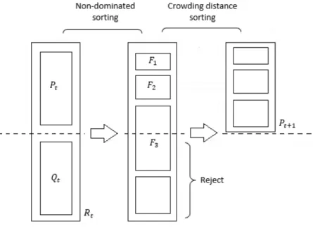
Non-dominated Sorting Genetic Algorithm II (NSGA-II), introduced by Deb et al. (2002), is an evolutionary algorithm that produces a set of the Pareto optimal solutions in one run. Has three principal components: elitist principle, emphasizes non-dominated solutions and explicit diversity preserving mechanism.

The NSGA-II procedure starts by creating a random populationP_t, of size N, and for each solution a in this population a value of the number of solutions that dominates it is created and is computed a set with all solutions dominated bya. For each solution is assigned a rank. Crossover and mutation operators are applied to this parent population

Figure 1: NSGA-II algorithm

to create a new pool of descendants Qt, of size N, which are mixed with the parents

population. This enlarged poolRt, with size 2N, is sorted into non-dominated fronts by

(17)

solutions from the last front have to be reject, then is applied the elitism method by adding a crowding distance to each solution to generate the next population Pt+1. This

distance, consider as being the density of individuals neighbouring a particular individual

a, is computed as the perimeter of the hypercube where the vertices are the nearby individuals to a. The crowding distance sorting assures diversity in the population and explores the ﬁtness landscape. The new populationPt+1 suﬀers crossover and mutation

to create a new descend population Qt+1, of size N and the NSGA-II algorithm is

repeated until the number of generations is reached.

(18)

3 Data and Methodology

In this section, we discuss the data collection as well as the procedure followed to optimize the investments of an insurance company. As a starting point we deﬁne the base scenario with an investment portfolio at the end of year 2015 and assess the solvency market capital requirements and the portfolio returns. The optimization process takes into account the maximization of the portfolio return to a minimization on the capital requirements.

3.1 Data Description

We consider the already built portfolio for a Non-life Insurance Company, that is composed with eight asset classes with a taxonomy set by the complementary identiﬁ-cation code (CIC): cash and deposits, collateralised securities, corporate bonds, equity, government bonds, investment funds, mortgages and loans and property.

(19)

3 Data and Methodology

Table 1: Asset classes of the portfolio Asset Classes

Cash and Deposits Corporate Bonds Collateralised Securities Equity Government Bonds Investment Funds Mortgage and Loans Property

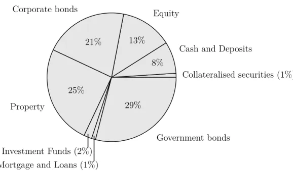
We have a total of 3535 assets and a total amount of investment of €339.26 millions. Our initial allocation is 7.85% for cash and deposits, 0.73% for collateralised securities, 20.76% for corporate bonds, 13.39% for equity, 29.38% for government bonds, 1.56% for investment funds, 1.32% for mortgage and loans and 25.28% for property.

Collateralised securities (1%) Cash and Deposits

8% Equity

13% Corporate bonds

21%

Property

25%

Investment Funds (2%) Mortgage and Loans (1%)

Government bonds 29%

Figure 2: Alocation of the amount invested in each asset class

(20)

the calculation of solvency capital requirements, equities have been separated in two types: type 1 are the equities listed in regulated markets in the countries which are members of the European Economic Area (EEA) or the Organisation for Economic Co-operation and Development (OECD) andtype2 are the equities listed in stock exchanges in countries which are not member of the EEA or the OECD, equities which are not listed, commodities and other alternative investments. The asset class of property has been divided into land and buildings (includes properties, plants and equipments held for own use and others than for own use) and real estate investment funds.

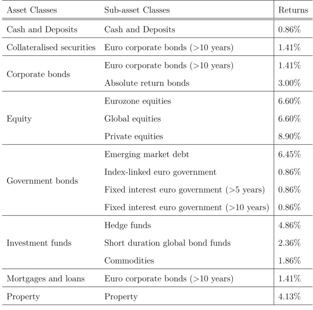
The assumption on expected returns of asset classes have been given by a consulting company and to map the classes of Solvency II (when diﬀerent) we split it into sub-classes. On government bonds we consider the bonds issued by less developed countries as emerging market debt1

and the others we divide by maturity: index-linked euro gov-ernment (<5 years), fixed interest euro govgov-ernment (<5 years) and fixed interest euro government (<10 years). Collateralised securities, mortgage and loans are considered as euro corporate bonds (>10 years) in our study. The equities that are not listed in a stock exchange and have CIC XL and XT are classified as private equities, the eurozone equities are issued by the countries from the Eurozone and all others are classified as global equities. Investment funds are split into hedge funds, commodities and short duration global funds (remaining funds). At last, corporate bonds are divided into euro corporate bonds (>10 years), that have maturity greater than ten years and are traded in Euro, and absolute return bonds that includes all others.

1

(21)

Asset Classes Sub-asset Classes Returns

Cash and Deposits Cash and Deposits 0.86%

Collateralised securities Euro corporate bonds (>10 years) 1.41%

Corporate bonds Euro corporate bonds (>10 years) 1.41%

Absolute return bonds 3.00%

Equity

Eurozone equities 6.60%

Global equities 6.60%

Private equities 8.90%

Government bonds

Emerging market debt 6.45%

Index-linked euro government 0.86% Fixed interest euro government (>5 years) 0.86% Fixed interest euro government (>10 years) 0.86%

Investment funds

Hedge funds 4.86%

Short duration global bond funds 2.36%

Commodities 1.86%

Mortgages and loans Euro corporate bonds (>10 years) 1.41%

Property Property 4.13%

Table 2: Expected returns of the asset classes (over 1 year horizon)

(22)

Absolute Return Bonds

18% Cash

8% Eurozone equities (1%)

Global Equities

6% Hedge Funds (1%)

Index-Linked euro government

29%

Private Equity 7%

Euro Corporate Bonds (>10yrs) 4%

Property 25%

Others (2%)

Figure 3: Alocation of the amount invested in each sub-asset class

We can then divide the total assets of the portfolio per sub-asset class.

Property Euro Corporate Bonds Absolute Return Bonds Eurozone Equities Global Equities Private Equities Emerging Market debt Index-Linked euro Government Fixed Interest euro Government >5 years Fixed Interest euro Government >10 years Hedge funds Short Duration global Bond Funds Commodities Cash 137 279 676 295 1 810 26 20 71 36 30 1 8 1 144

(23)

3.2 Methodology

3.2.1 Optimization Problem

Based on the assets chosen in each asset class shown on Table 1, we have a portfolio with a certain amount invested in each asset:

x= (x1, x2, ..., xn), (3.1)

with vectorxbeing the weight of each asset andn the number of assets in the portfolio. The total amount of investment should be divided amongst the n assets as

n X

i=1

x_i = 1 (3.2)

We can add other constraints by excluding short sales due to diﬃculties involved in shorting most of the asset types as well as to simplify the calculus:

x_i ≥0 (3.3)

Then, considering a bi-objective problem, that takes into account, simultaneously, the capital level for a non-life insurance company and the optimal investment portfolio on returns, we can state our objective function as:

    

   

maximize E[P]

minimize SCRM arket

(3.4)

3.2.2 Expected Profit

Having the weight invested in each sub-asset class, wi, and the respective returns,ri,

(24)

E[P] =X

i

wi.ri (3.5)

3.2.3 Market Risk Standard Formula

With the introduction of Solvency II, insurance companies were provided with a stan-dard formula for different risk types to calculate their solvency capital requirements (SCR), which is calibrated using the Value-at-Risk (Var) of the basic own funds (BOF) subject to a confidence level of 99.5 percent over a one year period (see Parliament and Union 2015).This study focus on the market risk module, which is a very relevant risk category in the insurance industry. European insurers are a major investor in Europe’s financial markets and market risk represents a relevant percentage of their solvency capital requirements (Ratings 2011).

Market risk module reflects the risk arising from the level or volatility of market prices of financial instruments which have an impact upon the level of the BOF of the undertaking. BOF is defined, mainly, as the difference between assets and liabilities on the economic balance sheet.

Market risk

Interest rate Equity Property Spread Currency Concentration

Figure 5: Market risk module and respective sub-modules.

(25)

Interestup = ∆BOF|up and Interestdown = ∆BOF|down (3.6)

The stress factors are applied to the basic risk-free interest rates as follows:

∆rup_t =rt(1 +supt )−rt and ∆rdownt =rt(1 +sdownt )−rt (3.7)

withsup_t and sdown

t being the interest rate shocks for up and down scenario andrt being

the basic risk-free rate for maturityt.

Equity risk arises from the risk of changes in the market prices of equities. All assets and liabilities whose value is sensitive to modiﬁcations in equities prices is exposed, but this sub-module only covers a downward stress scenario. The computation of this risk was based on the "standard" approach, with a symmetric adjustment mechanism (SAM), as (see Parliament and Union 2015):

Equity =qEquity21+ Equity 2

2+ 2×75%×Equity 2

1Equity 2 2,

Equityi = max (∆ BOF | equity shocki; 0).

(3.8)

withi∈ {1,2}and equity shock_i being an instantaneous increase in the value of equities classiﬁed as type 1 by 39% plus a SAM and being an instantaneous decrease in the value of equities classiﬁed as type 2 by 49% plus a SAM. This symmetric adjustment mechanism allows the equity shock to move within an interval of 10% on either side of the underlying standard equity stress.

The third sub-module, property risk, is the result of sensitiveness of assets, liabilities and ﬁnancial investments to the level or volatility of market prices of properties (see Parliament and Union 2015):

(26)

where property shock represents a decrease in the value of properties by 25%.

Changes in the credit worthiness of the issuers of the securities held in the insurer’s investment portfolio, that will be reﬂected in changes on the underlying credit spread, creates the spread risk (see Parliament and Union 2015):

Spread = Spreadbonds_{+ Spread}securisation_{+ Spread}derivatives_. _(3.10)

We do not consider the capital requirements for securisations and derivatives because of the available data.

Spreadbonds_{= max ( ∆}_BOF _|_{spread shock on bonds; 0)}_,

spread shock on bonds =X i

M VidurationiFup(ratingi),

(3.11)

where M V is the market value of asset i ∈ {1, ..., n}, Fup₍_rating

i) is a function of the

credit quality step of asset i and durationis the associated duration of asset i.

When investors are exposed to assets denominated in foreign currencies, face the risk of an adverse movement in the exchange rate of the denominate currency in relation to the base currency, known as currency risk (see Parliament and Union 2015):

Currencyup= max ( ∆BOF | currency upward schock; 0),

Currencydown _{= max ( ∆}_BOF _| _{currency downward schock; 0)}_,

(3.12)

with currency upward and downward shock being an instantaneous increase and an instantaneous decrease, respectively, of 25% of the value of the currency invested against the local currency.

(27)

Concentration =

s X

i

Conc2

i, (3.13)

whereConci is the risk charge for exposures to counterparty i and is deﬁned as:

Conci = ∆BOF | concentration downward shock,

concentration downward shock =XSi×gi,

XS_i = max (0;E_i−CT_i×Assets),

(3.14)

with XSi being the excess exposure to counterparty i, Ei denoting the exposure at

default to counterparty i, CTi denoting the relative concentration threshold applicable

to counterpartyi and gi being a reduction factor.

Then the total capital requirement for market risk is a combination of all the above sub-risks using a correlation matrix (see Parliament and Union 2015 ):

SCRmarket = s

X

i,j

Corri,jSCRiSCRj, (3.15)

wherei, j ∈ {interest, equity, property, spread, currency, concentration}andCorri,j

denotes the correlation matrix entry for the pair of risks (i, j).

3.2.4 Return on Risk-adjusted Capital

(28)

In RoRAC the capital is adjusted for risk and yields a financial analysis from the relationship between the expected profit and the risk capital necessary to achieve this profit (Matten and Warburg (1996)):

RoRAC = E[P]

SCRmarket

, (3.16)

(29)

4 Results

Considering the initial composition of a portfolio of a stylized Non-Life Insurance company we compute the values of the SCRmarket, E[P] and RoRAC.

Table 3: Solvency capital requirements for the market risk and expected proﬁt in mil-lions, and return on risk-adjusted capital of the initial portfolio

Risk i SCRi

Market €48.36

Interest rate €7.08 Equity €14.22 Property €19.96 Spread €6.24 Currency €1.34 Concentration €30.51

E[P] €1.72

RoRAC 0.036

(30)

4 Results

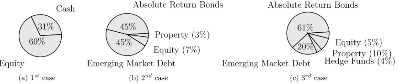
absolute return bonds, 45% on emerging market debt, 7% on equity and 3% on property. At last, as in Haslip (2011), we allocate our portfolio 61% on absolute return bonds, 5% on equity, 20% on emerging market debt, 4% on hedge funds and 10% on property.

Cash 31%

Equity 69%

(a) 1st

case

45%

Emerging Market Debt 45%

Equity (7%) Property (3%)

(b) 2nd

case

61%

Emerging Market Debt 20%

Hedge Funds (4%)Property (10%) Equity (5%)

(c) 3rd

case

Figure 6: Alocation of the amount invested in each sub-asset class for the three discrete cases

The results of this three allocations are as follow.

Table 4: Solvency capital requirements for the market risk and expected proﬁt in mil-lions, and return on risk-adjusted capital for the three discrete cases

1st _{case 2}nd _{case 3}rd _case

Risk i SCR_i SCR_i SCR_i

Market €68.08 €60.13 €46.89

Interest rate €9.23 €40.73 €12.60 Equity €51.50 €5.55 €7.81 Property €0 €2.37 €7.89 Spread €3.27 €24.99 €20.38 Currency €13.66 €1.39 €0.99 Concentration €31.79 €30.89 €31.38

E[P] €14.65 €6.66 €4.90

RoRAC 0.215 0.111 0.105

(31)

4 Results

asset allocation is possible to lower the capital at risk and to improve the returns of the company. Thus it is possible to set quantitative hypothesis to deﬁne a more proﬁtable investment strategy.

Using SolveXL software (Savić, Bicik, and Morley (2011)) to implement the multi-objective optimization on the initial portfolio, described on section 3, we can obtain a set of optimal asset allocation strategies.

A genetic algorithm (GA) maintains a large population of candidate solutions and each population is generated from its predecessor. Given that a GA is a stochastic search method, is diﬃcult for the solutions to satisfy equality constraints (Reid (1996)) and due to the complexity of the computations of the SCRmarket, on all following approaches

we do not impose a total investment restriction. Instead, we handle this restriction by reformulating the initial MOP, but we always maximize the expected proﬁt of the portfolio and minimize the capital requirements for market risk.

(32)

4 Results

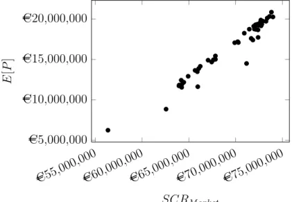
First we consider the initial MOP without any constraint.

        

max E[P]

min SCRmarket

(4.1)

After having the set of optimal solutions, we normalize the weight of each asset, dividing by their total sum. This way we fulﬁl the initial restriction that the total amount available must be invested.

A

C55,000

,000

AC60

,000,000

A

C65,000

,000

AC70

,000,000

A

C75,000

,000

A

C5,000,000

AC10,000,000

AC15,000,000

AC20,000,000

SCRM arket

E

[

P

]

Figure 7: Pareto front for the 1st _run

On the above ﬁgure, we have the Pareto optimal solutions for problem (4.1), where weights are normalized and the investment amount is, for all points, equal to €339.26 millions. On Figure 7, the values for the SCRmarket have had a signiﬁcant increase

compared with the initial value of €48.36 millions. Because we want to minimize the capital requirements for the market risk, the only solution to be consider is the strategy with the lower SCR_market.

Table 5: Result for the 1st _{run - investment,} _SCR

market and proﬁt in millions

Investment SCRmarket Proﬁt RoRAC

(33)

4 Results

From these procedure on, it would not be possible to normalize the weights of assets due to the nature of the optimization problem reformulations. Therefore, we have differ-ent investmdiffer-ent amounts and we consider the expected profit and the investmdiffer-ent amount as dependent values of the SRCmarket.

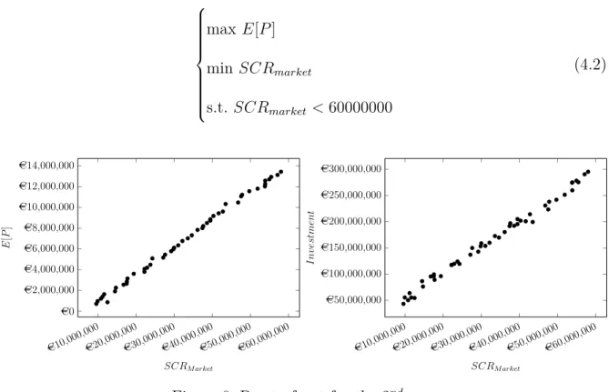
Since the values obtained, on problem (4.1), for the SCRmarket are higher than our

initial values, we make some adjustment to the MOP by subjecting the SCRmarket to

a risk target - be less than €48 millions. This leads to low investment amounts, with the higher amount being just €195.55 millions. Consequently, we increase the inequality constraint to €60 millions, to get higher values of investment.

                  

max E[P]

min SCRmarket

s.t. SCRmarket <60000000

(4.2) AC10 ,000,000 AC20 ,000,000 A C30,000 ,000 A C40,000 ,000 A C50,000 ,000 A C60,000 ,000 AC0 A

C2,000,000

A

C4,000,000

A

C6,000,000

A

C8,000,000

A

C10,000,000

A

C12,000,000

A

C14,000,000

SCRM arket

E [ P ] A C10,000 ,000 A C20,000 ,000 A C30,000 ,000 A C40,000 ,000 A C50,000 ,000 AC60 ,000,000 A

C50,000,000

A

C100,000,000

A

C150,000,000

A

C200,000,000

A

C250,000,000

A

C300,000,000

SCRM arket

I

nv

estment

Figure 8: Pareto front for the 2nd _run

(34)

4 Results

Table 6: Result for the 2nd _{run - investment,}_SCR

Investment SCR_market Proﬁt RoRAC €295.34 €58.04 €13.44 0.2316

To improve our investment strategy, we set higher ﬁgures for the investment amount, and introduce a new objective function - maximize the investment. To avoid that the solutions surpassed too much the initial amount, we impose a cap to this function of €400 millions. Also, we add a restriction for theSCRmarket to be less than €48 millions.

                                      

maxE[P]

min SCRmarket

maxInvestment

s.t.Investment <400000000

SCRmarket <48000000

(4.3)

AC5,000

,000

AC10

,000,000

A

C15,000

,000

AC20

,000,000

A

C25,000

,000

A

C30,000

,000

AC35

,000,000

A

C40,000

,000

AC45

,000,000

A

C50,000

,000

A C0 AC2,000,000 AC4,000,000 AC6,000,000 AC8,000,000

SCRM arket E [ P ] A

C5,000

,000

AC10

,000,000

A

C15,000

,000

A

C20,000

,000

AC25

,000,000

A

C30,000

,000

AC35

,000,000

A

C40,000

,000

A

C45,000

,000

AC50

,000,000

A C0 AC50,000,000 AC100,000,000 AC150,000,000 AC200,000,000 AC250,000,000 AC300,000,000 AC350,000,000 AC400,000,000

SCRM arket

I

nv

estment

Figure 9: Pareto front for the 3rd _run

(35)

4 Results

Table 7: Results for the 3rd _{run - investment,} _SCR

Investment SCR_market Proﬁt RoRAC €330.65 €43.32 €5.38 0.1241 €343.18 €46.83 €5.67 0.1212

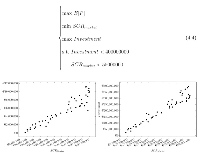
As can be seen on Figure 9, the risk target is limiting our solution space and the problem does not achieve the maximum value for the investment given the inequality constraint, therefore we increase the risk target toSCRmarket less than €55 millions.

                                      

maxE[P]

min SCRmarket

maxInvestment

s.t.Investment <400000000

SCRmarket <55000000

(4.4)

AC5,000

,000

AC10

,000,000

A

C15,000

,000

A

C20,000

,000

AC25

,000,000

A

C30,000

,000

A

C35,000

,000

AC40

,000,000

A

C45,000

,000

A

C50,000

,000

AC55

,000,000

AC0 AC2,000,000 AC4,000,000 AC6,000,000 AC8,000,000 AC10,000,000 AC12,000,000

SCRM arket E [ P ] A

C5,000

,000

A

C10,000

,000

A

C15,000

,000

AC20

,000,000

A

C25,000

,000

A

C30,000

,000

AC35

,000,000

AC40

,000,000

A

C45,000

,000

AC50

,000,000

AC55

,000,000

A C0 A C50,000,000 A C100,000,000 A C150,000,000 A C200,000,000 A C250,000,000 A C300,000,000 A C350,000,000 A C400,000,000

SCRM arket

I

nv

estment

Figure 10: Pareto front for the 5th _run

(36)

4 Results

Table 8: Results for the 5th _{run - investment,} _SCR

Investment SCRmarket Proﬁt RoRAC

€337.69 €49.78 €7.06 0.1419 €345.26 €47.97 €6.49 0.1353

Figures 7-10 suggests that there is an increasing, almost linear, relation between the

SCRmarket, the expected proﬁt and the investment value. As the amount of investment

increases, so are the variables for return and capital at risk. By imposing diﬀerent constraints and adding an objective function it is possible to have diﬀerent investment strategies that meet our objectives and that represent an improvement for the company. There are solutions where the SCRmarket has really low values, as can be seen on

Figure 8-10, but they are not worth to mention since it represents also low values of investment1

. For an insurance company that has an amount available to invest in a portfolio, investing less would mean that the diﬀerence would be anyway invested in cash, what could increase others risks of the standard formula, for example the counterparty risk.

We can resume our solutions to a set with six investment strategies.

Table 9: Summary of the optimal solutions - investment,SCRmarketand proﬁt in millions

Investment Strategy Set

Strategy no. Investment SCR_market Proﬁt RoRAC 1 €339.26 €56.36 €6.25 0.1109

2 €295.34 €58.04 €13.44 0.2316 3 €330.65 €43.32 €5.38 0.1241 4 €343.18 €46.83 €5.67 0.1212 5 €337.69 €49.78 €7.06 0.1419 6 €345.26 €47.97 €6.49 0.1353

1

(37)

4 Results

A RoRAC greater than one implies that the expected profit exceeds the market risk capital. In other words, per Euro risk capital a profit above one has been obtained. On Table 9, the highest RoRAC equals to 0.2316, meaning that per Euro risk capital a profit of 0.2316€ is achieved. The strategy number 2 grants more expected return of the portfolio for a less value of capital at risk, but it increases the capital requirements for the market risk at almost €10 millions and the expected profit at almost €12 millions. Also, by implementing this strategy the company would not invest the whole amount what implies an increase on other risks of the SCR. The second highest RoRAC is 0.1419 for strategy number 5, where we have a slightly increase of theSCRmarket and a substantial

increase of the proﬁts, compared to the initial values.

In view of improving the ﬁnancial position of the company, studying an allocation to minimize the market risk and to maximize the return, we do not consider strategy number 1. Thence, it has the lowest RoRAC and as can be noted on Table 9, there are strategies with a lower value of theSCRmarket and similar proﬁt. Strategies number 3,

4 and 6 yield a result lower than the initial strategy for the SCR_market and an increase of the proﬁt.

For the company to choose one of this investment strategies, should be taken into account the internal specifications of the company and its investment profile. First of all, must be considered that for all five strategies the investment value is different from the initial. When this difference is positive, it should be studied whether it is possible, or not, to transfer more money to be invested in the portfolio. When this difference is negative, the amount is anyway invested in cash, so it should be studied the impact this has on the remaining risks of the standard formula. To the strategies in which the SCRmarket is greater than the initial, which implies an increase in the SCR , it is

(38)

4 Results

the net income from investment returns. In addition to that, with the introduction of Solvency II , insurance companies must monitor, at all time, their solvency ratio which should be greater than 100% , ie, to put into practice the specified above strategies is necessary that the available capital funds the solvency capital requirement. A good strategy is to have a higher level for the solvency value, for example 150% , since it demonstrates the healthy financial situation of the company and because it is seen as a better protection against adverse events. At last, it depends on the weight given to each variable by the insurer, if it is more critical to reduce the SRC_market and not as much important to have an higher expected profit or higher RoRAC.

Figure 11 plots the allocations per sub-asset class of the five investment strategies considered. First, we notice that most portion of amount investment is allocated to Global Equities and Absolute Return Bonds. This can be explained by the fact that these sub-classes are composed by more assets and due to the reason that they have an higher rate of return comparing with the inital strategy. Investing a substantial amount in these two asset sub-classes allows a diversified investment policy, since they represent a large share of our portfolio (71%). On strategy number 2, there is a higher exposure to global equities, which justifies the amount for theSCRmarket, because we are increasing

(39)

4 Results

Global equities 83%

Absolute Return Bonds (9%) Others2

(8%)

(a) Strategy no. 2

35% Euro Corporate bonds (>10 years) (7%)

Eurozone Equities (4%) Fixed Interest euro govt Bonds (>10years) (4%)

Global equities

43% Index-Linked euro govts (AS) (3%) Others3

(8%)

(b) Strategy no. 3

Global equities 41%

Absolute Return Bonds 41% _{Euro Corporate bonds (}Others _>_{10 years) (9%)}

4

(9%)

(c) Strategy no. 4

33%

Global equities 52%

Cash (5%)Others

5

(5%)

Euro Corporate bonds (>10 years) (5%)

(d) Strategy no. 5

Absolute Return Bonds 37%

Euro Corporate bonds (>10 years) (6%) Fixed Interest euro govt Bonds (>10years) (3%)

Global equities

47% _Others6_(4%)

Eurozone Equities (3%)

(e) Strategy no. 6

Figure 11: Alocation of the amount invested in each sub-asset class for the ﬁve strategies

1

Euro Corporate Bonds (>10 years) (2%), Eurozone Equities (2%), Index-Linked Euro Government

(1%), Fixed Interest Euro Government Bonds (>10 years) (1%), Cash (1%), Others (1%)

2

Property (2%), Eurozone Equities (2%), Fixed Interest Euro Government Bonds (>5 years) (1%),

Cash (1%), Emerging Market Debt (2%)

3

Eurozone Equities (2%), Index-Linked Euro Government (2%), Fixed Interest Euro Government Bonds (>5 years) (1%), Fixed Interest Euro Government Bonds (>10 years) (2%), Cash (2%)

4

Eurozone Equities (1%), Index-Linked Euro Government (1%), Fixed Interest Euro Government Bonds (>10 years) (1%), Property (3%)

5

Index-Linked Euro Government (1%), Fixed Interest Euro Government Bonds (>5 years) (2%), Cash

(40)

5 Conclusions

In this paper we propose an approach to define an investment strategy for a stylized non-life insurance company. The procedure involves multi-objective optimization, to generate a set of investment strategies. We propose four problems to solve jointly for the optimal capital requirement and its optimal portfolio expected profit. Given equality constraints are hard to satisfy for a GA, we do not consider the restriction that the sum of the weighs invested must sum 1, but different reformulations of the initial problem. Each model is constructed based on the MOP to maximize the E[P] and minimize the SCRmarket. We begin by consider the initial optimization problem without any

constraint and we normalize the weigh of each asset to comply with the restriction that all the available amount must be invested. Based on the results, we then consider the problem with a restriction for theSCR_market value. The nature of the new optimization impossible the use of normalization, the same for the next two models. To overcome the diﬃculties of the investment amount we add another objective function - maximize the investment amount. For this models, we also consider a risk target for the SRCmarket,

with diﬀerent values, choose according to the results obtain.

(41)

5 Conclusions

Under Solvency II, when splitting the assets by the CIC there are ﬁfteen categories, and our study only contemplate eight classes. Therefore, future studies should include: Structured Notes, Futures, Call Options, Put Options, Swaps, Forwards and Credit Derivatives. Also, remaining risks of the standard formula use to compute the capital requirements of the company must be taken into account in setting the optimal SCR.

(42)

Bibliography

Asanga, Sujith et al. (2014). “Portfolio optimization under solvency constraints: a dy-namical approach”. In:North American Actuarial Journal 18.3, pp. 394–416. Asimit, Alexandru V et al. (2015). “Capital requirements and optimal investment with

solvency probability constraints”. In: IMA Journal of Management Mathematics

26.4, pp. 345–375.

Braun, Alexandru, Hato Schmeiser, and Florian Schreiber (2015a). “Maximizing the Return on Risk-Adjusted Capital: a Performance-Perspective Under S_olvency II_”. Extended Proposal.

Braun, Alexandru, Hato Schmeiser, and Florian Schreiber (2015b). “Portfolio optimiza-tion underS_olvency II _{constraints: implicit constraints imposed by the market risk} standard formula”. In:The Journal of Risk and Insurance.

Bruneau, Catherine and Sélim Mankai (2012). “Optimal Economic Capital and Invest-ment: Decisions for a Non-life Insurance Company”. In: Bankers, Markets and In-vestors/Banque et Marchés 119, pp. 19–30.

Deb, Kalyanmoy (2001).Multi-objective optimization using evolutionary algorithms. Vol. 16. John Wiley & Sons.

Deb, Kalyanmoy et al. (2002). “A fast and elitist multiobjective genetic algorithm: NSGA-II”. In:IEEE transactions on evolutionary computation 6.2, pp. 182–197. Dos Reis, Alfredo D. Egídio, Raquel M. Gaspar, and Ana T. Vicente (2010). “Solvency

(43)

Bibliography

Applications in Alternative Investing, Banking, Insurance, and Portfolio

Manage-ment, p. 267.

Duan, Yaoyao Clare (2007). “A Multi-objective Approach to Portfolio Optimization”. In:The Rose-Hulman Undergraduate Mathematics Journal 8.1.

Ehrgott, Matthias (2006).Multicriteria optimization. Springer Science & Business Me-dia.

EIOPA (2016). Risk-Free Interest Rate Term Structures. https://eiopa.europa.eu/

regulation- supervision/insurance/solvency- ii- technical- information/

risk-free-interest-rate-term-structures.

EIOPA (2014). The underlying assumptions in the standard formula for the Solvency Capital Requirement calculation.

EIOPA (2011). Report on the fifth Quantitative Impact Study (QIS5) for Solvency II. Elton, Edwin J. et al. (2014).Modern Portfolio Theory and Investment Analysis. ninth.

Wiley.

European Comission (2010).Quantitative Impact Study 5 Technical Specifications. Fischer, Katharina and Sebastian Schlütter (2012). Optimal investment strategies for

insurance companies in the presence of standardised capital requirements. Tech. rep. ICIR Working Paper Series.

Haslip, Gareth (2011). An Optimal Insurer in a Post S_olvency II _world_{. Tech. rep.} Liverpool: AON Benﬁeld.

Heckel, Tomas et al. (2012). Determining a strategic asset allocation in a S_olvency II

framework. Tech. rep. BNP Paribas Investments Partners.

(44)

Bibliography

Kaucic, Massimiliano and Roberto Daris (2015). “Multi-Objective Stochastic Optimiza-tion Programs for a Non-Life Insurance Company under Solvency Constraints”. In:

Risks 3.

Markowitz, Harry (1952). “Portfolio selection”. In:The journal of finance7.1, pp. 77–91. Matten, Chris and SBC Warburg (1996). Managing bank capital: capital allocation and

performance measurement. Wiley.

Parliament, The European and the council of the European Union (2009). “Directive 2009/138/EC OF THE EUROPEAN PARLIAMENT AND OF THE COUNCIL on the taking-up and pursuit of the business of Insurance and Reinsurance (Solvency II)”. In:Official Journal of the European Union.

Parliament, The European and the council of the european Union (2015). “Commission Delegated Regulation (EU) 2015/35 of 10 October 2014 supplementing Directive 2009/138/EC of the European Parliament and of the Council on the taking-up and pursuit of the business of Insurance and Reinsurance (Solvency II)”. In: Official Journal of the European Union.

Ratings, Fitch (2011). “Solvency II set to reshape asset allocation and capital markets”. In:Insurance Rating Group Special Report.

Reid, Darryn J (1996). “Genetic algorithms in constrained optimization”. In: Mathemat-ical and computer modelling 23.5, pp. 87–111.

Savić, Dragan A, Josef Bicik, and Mark Morley (2011). “A DSS generator for multiob-jective optimisation of spreadsheet-based models”. In: Environmental Modelling & Software 26.5, pp. 551–561.