D
D
R
R
I
I
V
V
E
E
R
R
S
S
O
O
F
F
P
P
R
R
I
I
V
V
A
A
T
T
E
E
C
C
O
O
N
N
S
S
U
U
M
M
P
P
T
T
I
I
O
O
N
N
I
I
N
N
T
T
H
H
E
E
E
E
R
R
A
A
O
O
F
F
F
F
I
I
N
N
A
A
N
N
C
C
I
I
A
A
L
L
I
I
S
S
A
A
T
T
I
I
O
O
N
N
:
:
N
N
E
E
W
W
E
E
V
V
I
I
D
D
E
E
N
N
C
C
E
E
F
F
O
O
R
R
T
T
H
H
E
E
E
E
U
U
R
R
O
O
P
P
E
E
A
A
N
N
U
U
N
N
I
I
O
O
N
N
C
C
O
O
U
U
N
N
T
T
R
R
I
I
E
E
S
S
Ricardo Barradas
D
D
e
e
z
z
e
e
m
m
b
b
r
r
o
o
d
d
e
e
2
2
0
0
1
1
7
7
W
W
P
P
n
n
.
.
º
º
2
2
0
0
1
1
7
7
/
/
0
0
4
4
DOCUMENTO DE TRABALHO WORKING PAPERDRIVERS OF PRIVATE CONSUMPTION IN THE ERA OF
FINANCIALISATION: NEW EVIDENCE FOR THE EUROPEAN
UNION COUNTRIES
1Ricardo Barradas
*
WP n. º 2017/04
DOI: 10.15847/dinamiacet-iul.wp.2017.041. INTRODUCTION ... 3
2. PRIVATE CONSUMPTION IN THE ERA OF FINANCIALISATION ... 5
3. ECONOMIC MODEL AND HYPOTHESES ... 9
4. DATA ... 13
5. ECONOMETRIC METHODOLOGY ... 15
6. EMPIRICAL RESULTS ... 17
6.1 ALL COUNTRIES AS A WHOLE ... 17
6.2 DIFFERENT GROUPS OF SIMILAR COUNTRIES ... 23
7. CONCLUSION... 26
8. REFERENCES ... 27
9. APPENDIX ... 34
1
D
D
R
R
I
I
V
V
E
E
R
R
S
S
O
O
F
F
P
P
R
R
I
I
V
V
A
A
T
T
E
E
C
C
O
O
N
N
S
S
U
U
M
M
P
P
T
T
I
I
O
O
N
N
I
I
N
N
T
T
H
H
E
E
E
E
R
R
A
A
O
O
F
F
F
F
I
I
N
N
A
A
N
N
C
C
I
I
A
A
L
L
I
I
S
S
A
A
T
T
I
I
O
O
N
N
:
:
N
N
E
E
W
W
E
E
V
V
I
I
D
D
E
E
N
N
C
C
E
E
F
F
O
O
R
R
T
T
H
H
E
E
E
E
U
U
R
R
O
O
P
P
E
E
A
A
N
N
U
U
N
N
I
I
O
O
N
N
C
C
O
O
U
U
N
N
T
T
R
R
I
I
E
E
S
S
ABSTRACT
This paper provides an empirical assessment of the effects of financialisation on private consumption using panel data for all 28 European Union countries from 1995 to 2015. According to the post Keynesian literature, financialisation exerts two contradictory effects on private consumption, notably a negative one linked to the fall of households’ labour income and a positive one related to the increase of households’ (financial and housing) wealth. A private consumption equation was estimated by including three variables linked to financialisation (labour income, financial wealth and housing wealth) and five additional control variables (lagged private consumption, short-term interest rate, long-term interest rate, inflation rate and unemployment rate). Our results confirm that financialisation has been detrimental to private consumption in the EU countries as a whole, and more specifically in the Euro area countries, as the beneficial wealth effect has not been sufficient to compensate for the prejudicial income effect. The fall of households’ labour income has even been the highest constraint on private consumption in the Euro area countries.
KEYWORDS
Private Consumption, Financialisation, Labour Income, Financial Wealth, Housing Wealth, European Union, Panel Data, Least-Squares Dummy Variable Bias-Corrected Estimator
JEL CLASSIFICATION
C23, D10, E21 and E441. INTRODUCTION
Over the last years and particularly until the Great Recession, private consumption has exhibited an increasing trend in many countries, occurring simultaneously with a general decreasing trend in households’ labour income. This ‘consumption without income’ hypothesis constitutes a kind of puzzle for the economic science, particularly because income tends to be regarded as the most important driver of private consumption.
Against this background, scholars of financialisation, adopting a post Keynesian view of point, stress that financialisation has been exerting a strong influence on the evolution of private consumption due to two conflicting channels (Stockhammer, 2009a; Onaran et al., 2011; and Hein, 2012). The first channel implicates a deceleration of private consumption caused by the decline of households’ labour income. The second channel involves an acceleration of private consumption caused by the growth of households’ (financial and housing) wealth.
Accordingly, the relationship between these two channels and private consumption has been tested by some empirical studies (Boone et al., 1998; Ludvigson and Steindel, 1999; Davis and Palumbo, 2001; Edison and Sløk, 2001; Ludwig and Sløk, 2001; Mehra, 2001; Boone and Girouard, 2002; Sousa, 2008 and 2009; Slacalek, 2009; Onaran et al., 2011; Barrell et al., 2015). Most of them derive and estimate private consumption equations by relating it to households’ labour income and households’ wealth following both permanent income and life-cycle theories of consumption (Friedman, 1957; Modigliani and Brumberg, 1954; Ando and Modigliani, 1963). The majority of these empirical studies find that labour income and (financial and housing) wealth exert a positive influence on private consumption, in a context where the positive effect of the latter more than compensates for the negative effect of the former. This seems to suggest that financialisation could represent by itself a potential response to the aforementioned puzzle surrounding the ‘consumption without income’ hypothesis.
This paper aims, therefore, to examine the role of financialisation in the evolution of private consumption in the European Union (EU) countries from 1995 to 2015, making a fivefold contribution to the existing literature. Firstly, the paper focuses on EU countries, for which the evidence is scarcer due to a strong emphasis on large and highly developed and financialised economies, like the US economy (Stockhammer, 2009a; Edison and Sløk, 2001). EU countries represent an interesting case by presenting a certain institutional diversity despite belonging to the same economic and political region. Secondly, the paper performs a panel data econometric analysis, whilst the majority of empirical studies on this subject perform a time series econometric analysis (Boone et al., 1998; Ludvigson and Steindel, 1999; Davis and Palumbo, 2001; Edison and Sløk, 2001; Mehra, 2001; Boone and Girouard, 2002; Sousa, 2008
and 2009; Onaran et al., 2011; Barrell et al., 2015). Note that a panel data econometric analysis offers several advantages with the possibility to collect a higher number of observations with more variability and less collinearity, which improve the accuracy and the reliability of estimations (Baltagi, 2005; Brooks, 2009). Thirdly, the paper assesses the period before, during and after the crisis, whereas the existing literature typically is focused on the period prior to the Great Recession. Barrell et al. (2015) is the only exception, but they only analyse Italy and the UK individually though a time series econometric analysis. Fourthly, this paper evaluates the effects of financialisation on total and on all the components of private consumption (consumption of services and consumption of non-durable, semi-durable and durable goods), which is a novelty to the literature. Fifthly, the paper estimates a private consumption equation by including other control variables in order to take into account other important determinants of private consumption (Church et al., 1994; Boone et al., 1998; Davis and Palumbo, 2001; Boone and Girouard, 2002) and mitigate the risk of potential inconsistent and unbiased estimations due to the problem of omitted relevant variables (Wooldridge, 2003; Kutner et al., 2005; Brooks, 2009).
Thus, a private consumption equation is estimated using three variables linked to financialisation (labour income, financial wealth and housing wealth) and five additional control variables (lagged private consumption, short-term interest rate, long-term interest rate, inflation rate and unemployment rate). Estimations are produced using the least-squares dummy variables bias-corrected estimator (LSDVC) due to the existence of a dynamic panel data model, an unbalanced panel and a macro panel.
The paper concludes that financialisation has been prejudicial to private consumption in the EU countries as a whole, and more specifically in the Euro area countries, because the positive wealth effect has not been sufficient to compensate for the negative income effect. The fall of households’ labour income has even been the highest constraint on private consumption in the Euro area countries.
The remainder of the paper is organised as follows. Section 2 presents a review of literature on the effects of financialisation on private consumption. In Section 3, a private consumption equation is presented, as well as the expected effects of each variable included in that equation. Data and methodology are described in Sections 4 and 5, respectively. In Section 6, we present the main results and the concomitant discussion. Finally, Section 7 concludes.
2. PRIVATE CONSUMPTION IN THE ERA OF FINANCIALISATION
It is widely accepted that understanding the determinants of private consumption is a central topic in economic science, notably because private consumption tends to be the most important component of aggregate demand and makes a strong contribution to gross domestic product (GDP) in several countries, therefore playing a crucial role in economic growth.Against this backdrop, scholars on financialisation have claimed that the emergence of this phenomenon has had profound effects on households’ consumption since the mid-1980s due to their higher engagement in the realm of financial markets either as debtors (especially through credit) and/or asset holders (housing, pensions, insurance, money market funds and other financial assets) (Stockhammer, 2010; Lapavitsas, 2011; Barradas, 2016).2 This behaviour has been transversal to the generality of households, including low-income and middle-class households (Van der Zwan, 2014).
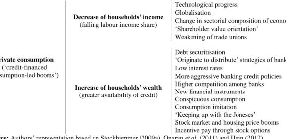
Indeed, the evolution of private consumption in the last years cannot be dissociated from the process of financialisation. Framed in the post Keynesian tradition, it is argued that financialisation has originated two contradictory effects on private consumption (Stockhammer, 2009; Onaran et al., 2011; and Hein, 2012). Figure 1 illustrates the two channels (and factors that contribute to explain each of them) associated with these contradictory effects of financialisation on private consumption.
Figure 1 – The channels associated to the contradictory effects of financialisation on private consumption
Private consumption
(‘credit-financed consumption-led booms’)
Decrease of households’ income
(falling labour income share)
Technological progress Globalisation
Change in sectorial composition of economies ‘Shareholder value orientation’
Weakening of trade unions
Increase of households’ wealth
(greater availability of credit)
Debt securitisation
‘Originate to distribute’ strategies of banks Low interest rates
More aggressive banking credit policies Higher competition among banks New financial instruments Conspicuous consumption Consumption imitation ‘Keeping up with the Joneses’ Stock market and housing price booms Incentive pay through stock options
Source: Authors’ representation based on Stockhammer (2009a), Onaran et al. (2011) and Hein (2012)
2 Note that these authors also provide a detailed analysis on the effects of financialisation on the
remaining economic agents (non-financial corporations, financial corporations and policy makers). Here, we focus only on households given our interest in analysing the drivers of private consumption in the era of financialisation.
The first channel is linked with the fall (rise) of the labour income (profit) share in the era of financialisation (Stockhammer, 2009, 2012 and 2017; Kristal, 2010; Dünhaupt, 2011; Peralta and Escalonilla, 2011; Estrada and Valdeolivas, 2012; Lin and Tomaskovic-Devey, 2013; Barradas, 2017; Barradas and Lagoa, 2017), which puts a downward pressure on private consumption through the reduction of households’ labour income. This happens because wage incomes are normally related to higher consumption propensities than profit incomes (Stockhammer, 2012).
Several reasons can be identified in the literature for the fall of the labour income share. The most important ones are technological progress (European Commission, 2007; Stockhammer, 2009; Guerriero and Sen, 2012; Dünhaupt, 2013b), globalisation (European Commission, 2007; Guerriero and Sen, 2012; Dünhaupt, 2013b) and financialisation (Hein, 2012; Hein and Detzer, 2014; Michell, 2014; Hein and Dodig, 2015). According to these latter authors, financialisation exerts a negative influence on the labour income share though three different channels: the change in the sectorial composition of economies (visible in the increasing importance of financial activity and the decreasing importance of general government activity), the emergence of ‘shareholder value orientation’ and the deterioration of general workers’ bargaining power through the weakening of trade unions. Stockhammer (2009 and 2017), Kristal (2010), Peralta and Escalonilla (2011), Dünhaupt (2013a), Lin and Tomaskovic-Devey (2013), Alvarez (2015), Köhler et al. (2016), Barradas (2017) and Barradas and Lagoa (2017) are good examples of empirical econometric studies on the impact of financialisation on the labour income share. Most of them find it to be harmful.
The second channel is related to a higher availability of credit in the era of financialisation, which puts an upward pressure on private consumption through the increase of (notional or virtual) households’ wealth at the expense of higher indebtedness. This greater availability of credit could be explained by financial innovation (e.g., debt securitisation and the ‘originate to distribute’ strategies of banks) in an environment of low interest rates, resulting in a deterioration of creditworthiness standards and making credit increases available even for low-income and low-wealth households (Hein, 2012). Stockhammer (2009) also adds that banks have followed more aggressive credit policies, giving households greater access to credit, not only restricted to mortgages, but also other forms of consumer credit, credit cards and overdraft bank accounts (with small penalty and/or without any penalty) in a context of increasing competition among financial institutions (Boone and Girouard, 2002). Credit has also been stimulated by the appearance of new financial instruments, like home equity loans and the aforementioned credit cards (with high plafond and/or without any plafond). Against this
backdrop, households could mitigate the fall in their wages, feed conspicuous consumption and follow a consumption imitation of Veblen and other goods by ‘keeping up with the Joneses’ (Hein, 2012).3
As a result, households’ indebtedness has been increasing considerably in the era of financialisation, in a context where it is increasingly difficult to assess whether such indebtedness is due to households’ rational decisions and whether it is sustainable or not. On the one hand, wage stagnation seems to be counter-productive with the maintenance of consumption levels by households, namely with the rise of consumption using credit cards (Stockhammer, 2009). On the other hand, stock market and housing price boom episodes have each increased (notional or virtual) wealth against which households were willing to borrow (Hein, 2012). The high levels of households’ indebtedness tend to increase financial fragility by making economies more vulnerable to any downside risks.
The increase of households’ wealth could be also associated with the proliferation of incentive pay to employees in the form of stock options in addition to cash not only in the USA, but also in other EU countries (Edison and Sløk, 2011).
Despite these two conflicting effects of financialisation on private consumption, the beneficial role of the increase of households’ wealth (second channel) has more than compensated for the prejudicial effect of the decrease of households’ labour income (first channel), stressing that the global effect of financialisation on private consumption has been positive in the era of financialisation (Stockhammer, 2009; Onaran et al., 2011; Hein, 2012). This seems to provide an explanation for the puzzle identified in several countries: the existence of a trend of higher consumption along with lower labour income (‘consumption without income’ hypothesis).4
These countries are experiencing therefore ‘credit-financed consumption-led booms’. EU countries are a good example to verify this hypothesis due to the increasing trends of consumption and (financial and housing) wealth along with the decreasing trend of income in the last years and especially until the Great Recession (Figure A1 to Figure A4 in the Appendix).
3 This is the so-called ‘demonstration effect’ or ‘Duesenberry effect’, according to which households imitate
or copy the consumption levels of their neighbours or other households (Duesenberry, 1949).
4 This trend of higher consumption along with lower income could also be interpreted as a ‘ratchet effect’
(Duesenberry, 1949). According to this author, this means that when there is a decline in households’ income, private consumption does not decline much because households try to maintain their consumption at the highest level attained before the fall of their incomes for two reasons. Firstly, this happens because households are accustomed to their previous standard of living. Secondly, this happens because, due to the aforementioned ‘demonstration effect’, households are not willing to show to the other households that they lost their previous standard of living.
From an econometric view point, some empirical studies estimate consumption functions in order to assess financialisation’s impact on private consumption by relating it to households’ labour income and households’ wealth (e.g., Boone et al., 1998; Ludvigson and Steindel, 1999; Davis and Palumbo, 2001; Edison and Sløk, 2001; Ludwig and Sløk, 2001; Mehra, 2001; Boone and Girouard, 2002; Sousa, 2008 and 2009; Slacalek, 2009; Onaran et al., 2011; Barrell et al., 2015). As noted by Boone and Girouard (2002), this approach rests on permanent income and life-cycle theories of consumption, where private consumption depends on households’ permanent income, i.e., the current and expected future labour income plus their stock of (financial and housing) wealth (Modigliani and Brumberg, 1954; Friedman, 1957; Ando and Modigliani, 1963). Most of these empirical studies find that labour income and (financial and housing) wealth exert a positive influence on private consumption.
Despite the strong variety of econometric empirical studies on this issue, five characteristics are transversal across most of them. Firstly, they are strongly focused on large and highly developed and financialised economies and particularly the US economy. In addition, Stockhammer (2009) still warns that this econometric evidence for the US economy is often based on a short period of observations and reinforces that the evidence for the EU countries is relatively scarce. This is also reinforced by Edison and Sløk (2001) who reiterate that econometric empirical studies covering the EU countries are rather limited. There are several exceptions but they are often confined to the G7 countries (e.g., Boone et al., 1998; Boone and Girouard, 2002; Barrell et al., 2015). Secondly, they perform time series econometric analysis by assessing the relationship between financialisation and private consumption in specific countries. Ludwig and Sløk (2001) and Slacalek (2009) are the only exceptions by ascertaining the financial and housing wealth effects for a panel of 16 countries as a whole and for both ‘market-based’ and ‘bank-based’ countries separately. Thirdly, they only consider the pre-2007 crisis period. The study by Barrell et al. (2015) is the only one that takes into account the recent financial and economic crisis on their estimates, but they are only focused on Italy and the UK. Fourthly, they only estimate the effects of financialisation on private consumption of non-durable goods by considering that consumption of durable goods represents additions and replacements to asset stocks (Ludwig and Sløk, 2001; Mehra, 2001; Barrell et al., 2015). Fifthly, they do not include other (control) variables beyond households’ labour income and households’ wealth in their consumption functions, neglecting other important determinants of private consumption such as income uncertainty, substitution effects, depreciation of non-indexed financial assets, among others (Church et al., 1994; Boone et al., 1998; Davis and Palumbo, 2001; Boone and Girouard, 2002). This highlights the risk of
potential inconsistent and unbiased estimates due to the problem of omitted relevant variables (e.g., Wooldridge, 2003; Kutner et al., 2005; Brooks, 2009).
Against this backdrop, this paper aims to conduct an empirical assessment of the relationship between financialisation and private consumption conducting a panel data econometric analysis for the EU countries from 1995 to 2015 using macroeconomic annual data. Our work extends, therefore, the previous research in several directions and aims to circumvent the aforementioned main caveats identified in the literature, namely by analysing the EU countries; performing a panel data econometric analysis; incorporating the period before, during and after the crisis; assessing the effects of financialisation on private consumption by durability (consumption of services; consumption of non-durable, semi-durable and durable goods; and all of them); and estimating a consumption function with other control variables.
3. ECONOMIC MODEL AND HYPOTHESES
In what follows, we estimate a private consumption equation by including two different groups of variables. Firstly, we include three variables linked to the channels related to the two
conflicting effects of financialisation on private consumption and which are typically used in econometric empirical studies on this matter: labour income, financial wealth and housing wealth. Secondly, we incorporate five control variables that normally are also recognised as important drivers of private consumption: lagged private consumption, short-term interest rate, long-term interest rate, inflation rate and unemployment rate.
Accordingly, our consumption equation takes the following form:
(1)
where i is the country, t is the time period (years),
C
is the private consumption of country i at time t,LI
is the households’ labour income of country i at time t,FW
is the households’financial wealth of country i at time t,
HW
is the households’ housing wealth of country i at time t,SIR
is the short-term interest rate of country i at time t,LIR
is the long-term interest rate of country i at time t,INF
is the inflation rate of country i at time t andUR
is the unemployment rate of countryi
at timet
.The two-way error term component is given by:
(2) t , i t i t , i 0 1 i,t1 2 i,t 3 i,t 4 i,t t , i C LI FW HW C
t , i t , i 8 t , i 7 t , i 6 t , i5
SIR
LIR
INF
UR
where i accounts for unobservable country-specific effects and t accounts for time-specific effects. The term i,t is the random disturbance in the regression, varying across countries and years.
We include the lag of the dependent variable, taking into account the degree of persistence that is exhibited by private consumption. This consumption inertia or sluggishness is associated with the existence of consumption habits by households according to the framework of habit formation or with the existence of households that are unaware of macroeconomic news according to the framework of sticky expectations (Sommer, 2007; Slacalek, 2009; Barrell et al., 2015). Sousa (2009) also highlights the adjustment costs of changing consumption, evaluation of finances only at periodic intervals and inattention as other potential sources of consumption inertia. Indeed, Sørensen and Whitta-Jacobsen (2005) highlight the strong persistence of private consumption as a stylised fact of business cycles.
Similar to the other aforementioned econometric empirical studies, we are proposing to estimate an aggregate consumption function. This approach implicitly entails the assumption of the existence of a representative household, which introduces some limitations in the assessment of our results notably because we are interested in analysing a macroeconomic issue – i.e., drivers of private consumption – but the theory of household spending is supported by microeconomic fundamentals. Firstly, it prevents the assessment of determinants of private consumption from households with different income levels and wealth levels and from different countries. Secondly, it underestimates the historical, social and economic environments responsible for the evolution of private consumption in each country because a panel data econometric analysis estimates an average effect of several countries. In this paper, a macroeconomic perspective is followed allowing us to look beyond the specificities of each household and to ascertain the main relationships that dominate private consumption. Thus, if the two channels of financialisation are found to have a macroeconomic effect on private consumption, we cannot conclude whether it is due to the impact of some households/countries or is transversal to all households/countries. If the two channels are found to not have any macroeconomic effect, we cannot exclude that they affect a subset of households/countries, which, however, is not enough to create a macroeconomic effect on private consumption in all EU countries.
Regarding the effect of each variable on private consumption, lagged private consumption, labour income and financial wealth are expected to impact positively, whilst inflation rate and unemployment rate are expected to impact negatively. Housing wealth and
interest rate could positively or negatively impact private consumption. Therefore, coefficients of these variables are expected to have the following signs:
(3)
The labour income is expected to exert a positive impact on private consumption following a Keynesian argument. According to Keynes (1936), the respective coefficient is less than one, given the idea that households increase their consumption as their income increases, but not as much as the increase in their income.
Financial wealth is expected to positively impact private consumption due to five different transmission mechanisms (Ludwig and Sløk, 2001). The first mechanism is the ‘realised wealth effect’, according to which the increase in the value of financial assets tends to spur private consumption when households decide to realise their gains by liquidating them (Boone and Girouard, 2002). The second mechanism is the ‘unrealised wealth effect’, which means that the increase in the value of financial assets tends to spur private consumption because households feel more confident. They believe that this increasing trend in financial assets could persist in the future, so they will consume more due to expectations that their income and wealth will be higher in the future when they realise those gains. The ‘liquidity constraints effect’ represents the third mechanism. Here, private consumption increases due to the rise in the value of households’ portfolios that can be used as collateral for new borrows.5
The fourth mechanism is the so-called ‘stock option value effect’, which is associated with an acceleration of consumption as a result of an increase in the value of households’ stock options. The fifth mechanism is the rise of private consumption by households that do not participate in financial markets but that are also affected by changes in these asset prices (Romer, 1990).
Housing wealth has an ambiguous effect on private consumption (Ludwig and Sløk, 2001). These authors suggest that three mechanisms explain a positive relationship between housing wealth and private consumption. The first one is also the ‘realised wealth effect’, in a context where the increase in house prices leads to a rise in net wealth of households that are house owners because they can take out equity in the form of refinancing or selling the house, which tends to raise private consumption. The second mechanism is the ‘unrealised wealth effect’, according to which a rise in house prices raises private consumption even though households do not refinance or sell the house. The idea is that households feel more confident,
5 This rests on the financial accelerator theory developed by Bernanke et al. (1996), which stresses that
asset price inflation tends to raise collateral values, which allows for more borrowing to finance consumption and/or investment.
spending more today given such expectations that they are richer than they were before the increase of house prices. The third mechanism is the ‘liquidity constraints effect’, which is related to the utilisation of housing as collateral for new loans. This indicates that a surge in housing prices have a positive impact on housing wealth, supporting a wish for more loans that boosts private consumption. Nonetheless, they also emphasise that there are two further mechanisms explaining a negative relationship between housing wealth and private consumption. The first one is the ‘budget constraint effect’, which describes that an increase in housing prices has a negative impact on private consumption by households that are renters due to the expected increase of rents and by households that are owners due the expected increase of other housing services such as fuel and power. In addition, Boone and Girouard (2002) also note that house owners do not feel wealthier when there is a rise in housing prices because their implicit rental costs also increase. The second mechanism is the ‘substitution effect’, which occurs when households that are planning to buy a house respond to a surge in house prices by buying a smaller house or lowering private consumption.
The level of short-term and long-term interest rates has an undetermined effect on private consumption, reflecting the classical view around the so-called substitution and income effects between saving and consumption. The substitution effect shows that a rise in the level of interest rates stimulates savings due to higher rates of return, which impairs private consumption because it becomes relatively less attractive to hold cash and/or to spend. The income effect is related with returns received by savers from their savings. Thus, an increase of interest rates initiates a rise in incomes received by savers, which can stimulate private consumption if they channel these incomes to spend more and if they think that they do not need to save as much to maintain the level of their savings.
The inflation rate is expected to exert a negative influence on private consumption, functioning as a proxy for the uncertainty and for the real depreciation of non-indexed financial assets (Boone et al., 1998; and Boone and Girouard, 2002).
In addition, private consumption also depends negatively on the unemployment rate, because its fluctuations tend to mirror the business cycle by operating therefore as proxy for uncertainty regarding future income levels (Boone et al., 1998; Boone and Girouard, 2002). This is confirmed by Malley and Moutos (1996), who claim that unemployment is a valuable measure of income uncertainty. They also state that an increase in income uncertainty induces more saving (less consumption) due to precautionary motives.
4. DATA
Annual data was collected from 1995 to 2015 for all EU countries. This corresponds to the period and frequency for which all data are available, which does not compromise the appropriateness of our sample to undertake our study because we cover the period when financialisation gained more influence (van der Zwan, 2014). Table 1 shows the structure of our sample.
Table 1 – Sample composition
Country Period Observations Missing
Austria 2001-2015 15 6 Belgium 1995-2015 21 0 Bulgaria 2006-2015 10 11 Cyprus 2003-2015 13 8 Czech Republic 2009-2015 7 14 Denmark 1995-2015 21 0 Estonia 2006-2010 5 16 Finland 1995-2015 21 0 France 1995-2015 21 0 Germany 1995-2015 21 0 Greece 1998-2015 18 3 Hungary 2008-2015 8 13 Ireland 2001-2015 15 6 Italy 1995-2015 21 0 Latvia 2007-2015 9 12 Lithuania 2001-2015 15 6 Luxembourg 2008-2015 8 13 Malta 2004-2015 12 9 Netherlands 1995-2015 21 0 Norway 1995-2015 21 0 Poland 2011-2015 5 16 Portugal 1995-2015 21 0 Romania 2010-2015 6 15 Slovakia 2006-2015 10 11 Slovenia 2008-2015 8 13 Spain 1995-2015 21 0 Sweden 1995-2015 21 0 United Kingdom 1995-2015 21 0
Against this backdrop, we obtained panel data including a total of 28 cross-sectional units (N27) observed over time from 1995 to 2015 (
T
21
). Due to lack of available data, we obtained an unbalanced panel because it was impossible to collect data for all the variables for all the years for each country. Our unbalanced panel includes a total of 416 observations and 172 missing values.Now we present the definitions and sources for all variables used in our study. Private consumption is proxied by the ratio between the final consumption expenditure of households and the GDP at market prices. These two variables were collected from the European national accounts at current prices and in millions of national currency, available from Eurostat.
The proxy for labour income is the adjusted labour share, available from the AMECO database. This variable reflects the ratio between the compensation of employees per employee and the GDP at current market prices per employee. This is the traditional variable used to measure labour income because it allows including both dependent and self-employed workers, treating earnings of these workers as labour income (Dünhaupt, 2013a).
We used the financial assets of households and non-profit institutions serving households as a percentage of GDP at market prices to measure financial wealth. These two variables were collected from European financial accounts and European national accounts, respectively, at current prices and in millions of national currency, available from Eurostat.
Housing wealth is assessed by the annual growth rate of the nominal housing price index from the analytical house prices indicators, available from the OECD database. When not available on the OECD database, observations of this variable were obtained from the annual growth rate of the nominal housing price index, available from the Eurostat database and Bank for International Settlements database. This is the only housing wealth related variable available for our sample due to the lack of data regarding the non-financial assets owned by households. However, house prices have been used by other authors to measure housing wealth, who reinforce that this is a good proxy (Boone et al., 1998; Ludwig and Sløk, 2002).
We also used both short-term and long-term nominal interest rates from the AMECO database. Interest rates for Norway were obtained from monetary and financial statistics on the OECD database.
The inflation rate used here corresponds to the annual growth rate of the price deflator of the GDP at market prices (2010=100), available from the AMECO database.
Finally, the unemployment rate is measured by the number of unemployed as a percentage of the active population and it was collected from the Labour force survey on the Eurostat database.
Note that our variables are expressed as ratios (private consumption, labour income, financial wealth and unemployment rate) or growth rates (housing wealth and inflation rate). This approach has a twofold advantage, notably by allowing the use of variables from different countries that are expressed in different currencies and by facilitating the interpretation of the respective coefficients.
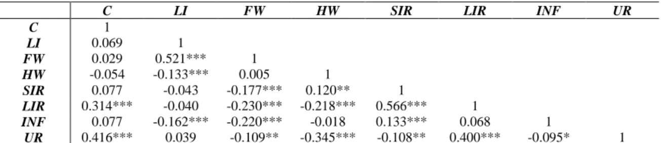
Table 2 – The correlation matrix
C LI FW HW SIR LIR INF UR
C 1 LI 0.069 1 FW 0.029 0.521*** 1 HW -0.054 -0.133*** 0.005 1 SIR 0.077 -0.043 -0.177*** 0.120** 1 LIR 0.314*** -0.040 -0.230*** -0.218*** 0.566*** 1 INF 0.077 -0.162*** -0.220*** -0.018 0.133*** 0.068 1 UR 0.416*** 0.039 -0.109** -0.345*** -0.108** 0.400*** -0.095* 1
Note: *** indicates statistical significance at 1% level, ** indicates statistical significance at 5% level and * indicates statistical significance at 10% level
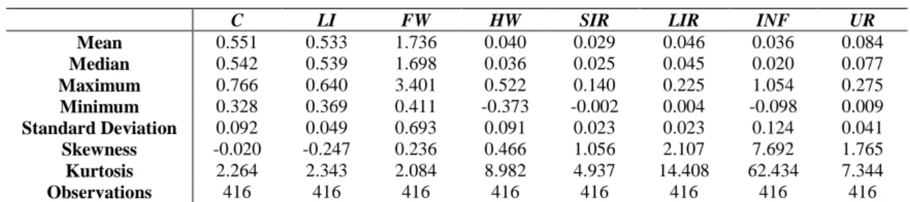
Table A1 in the Appendix contains the descriptive statistics for each variable and Table 2 presents the correlation matrix between variables. The most important finding is the non-existence of significant multicollinearity between variables because all correlation coefficients are lower than the traditional ceiling of 0.8 in absolute terms (Studenmund, 2005).
5. ECONOMETRIC METHODOLOGY
As described in the previous two Sections, we use a dynamic panel data model due to the incorporation of a lagged dependent variable among the independent variables, an unbalanced panel due to the existence of missing values in our sample and a macro panel due to the moderate cross-sectional dimension
N
. Under these circumstances, we will employ the LSDVC estimator (Nickel, 1981; Bun and Kiviet, 2003; Bruno, 2005a and 2005b) following the ‘xtlsdvc’ instruction from the Stata software.Three aspects can be enumerated to justify the suitability of the LSDVC estimator taking into account the aforementioned characteristics of our panel. The first is related with the biased and inconsistent estimates produced by the standard panel data estimators (e.g., pooled ordinary least-squares, least-squares dummy variables, fixed-effects and random effects), notably because the lagged dependent variable is correlated with fixed effects in the error term (Nickel, 1981; Baltagi, 2005; Cameron and Trivedi, 2009). The second is also associated with the severely biased and imprecise estimates produced by the standard panel data estimators for dynamic panel data models (e.g., Anderson and Hsiao, 1982; Arrelano and Bond, 1991; Arrelano and Bover, 1995; Blundell and Bond, 1998), mainly when we have a macro panel with a relatively small cross-sectional dimension
N
(Bruno, 2005a and 2005b). The third is linked with the Monte Carlo experiments on the outperformance of the LSDVC estimator vis-à-vis theaforementioned estimators in terms of bias and root mean squared errors in the case of macro panels (Kiviet, 1995; Judson and Owen, 1999; Bruno, 2005a and 2005b).
Note that the estimates produced by the LSDVC estimator are obtained in two steps (Bruno, 2005a and 2005b). The first step corresponds to the production of consistent estimates, which needs the definition of an initial matrix of starting values through the execution of one of three consistent estimators (Anderson and Hsiao, 1982; Arrelano and Bond, 1991; Blundell and Bond, 1998). The second step is the correction of the bias through the realisation of a set of multiple replications to bootstrap the standard errors. However, the produced estimates are not significantly affected either by the choice of one consistent estimator in the first step or by the choice of the number of replications in the second step (Bun and Kiviet, 2001; Bruno, 2005a and 2005b).
Against this background, our estimates are presented in the next Section where we use Arrelano and Bond’s (1991) estimator in the first step and a number of replications equal to 250 in the second step. Time dummies are included, as well as WALD tests to evaluate the statistical significance of them.
6. EMPIRICAL RESULTS
6.1 ALL COUNTRIES AS A WHOLE
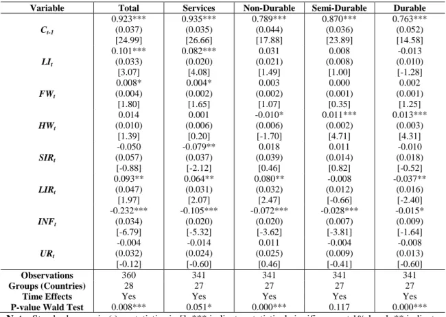
Our estimates are presented in this Subsection, where we begin with the results for the entire sample. Estimates are carried out not only for total private consumption but also for the different components of private consumption by disaggregating it by durability. This allows us to better understand the determinants of private consumption in the era of financialisation in the EU countries as a whole. Results are illustrated in Table 3.
Table 3 – Estimates of private consumption by durability for full period (1995-2015) Variable Total Services Non-Durable Semi-Durable Durable
Ct-1 0.923*** (0.037) [24.99] 0.935*** (0.035) [26.66] 0.789*** (0.044) [17.88] 0.870*** (0.036) [23.89] 0.763*** (0.052) [14.58] LIt 0.101*** (0.033) [3.07] 0.082*** (0.020) [4.08] 0.031 (0.021) [1.49] 0.008 (0.008) [1.00] -0.013 (0.010) [-1.28] FWt 0.008* (0.004) [1.80] 0.004* (0.002) [1.65] 0.003 (0.002) [1.07] 0.000 (0.001) [0.35] 0.002 (0.001) [1.25] HWt 0.014 (0.010) [1.39] 0.001 (0.006) [0.20] -0.010* (0.006) [-1.70] 0.011*** (0.002) [4.71] 0.013*** (0.003) [4.31] SIRt -0.050 (0.057) [-0.88] -0.079** (0.037) [-2.12] 0.018 (0.039) [0.46] 0.011 (0.014) [0.82] -0.010 (0.018) [-0.52] LIRt 0.093** (0.047) [1.97] 0.064** (0.031) [2.07] 0.080** (0.032) [2.47] -0.008 (0.012) [-0.66] -0.037** (0.016) [-2.40] INFt -0.232*** (0.034) [-6.79] -0.105*** (0.020) [-5.32] -0.072*** (0.020) [-3.62] -0.028*** (0.007) [-3.81] -0.015* (0.009) [-1.64] URt -0.004 (0.032) [-0.12] -0.014 (0.024) [-0.60] 0.011 (0.025) [0.46] -0.004 (0.009) [-0.41] -0.008 (0.013) [-0.60] Observations 360 341 341 341 341 Groups (Countries) 28 27 27 27 27
Time Effects Yes Yes Yes Yes Yes
P-value Wald Test 0.008*** 0.051* 0.000*** 0.117 0.000***
Note: Standard errors in ( ), z-statistics in [], *** indicates statistical significance at 1% level, ** indicates statistical significance at 5% level and * indicates statistical significance at 10% level. Coefficients, standard errors and z-statistics for the year dummies are not reported
With regard to total private consumption, all the variables are statistically significant at the traditional significance levels with the exception of housing wealth, short-term interest rates and unemployment rate. Note that results do not change substantially if we had used the real house prices instead of the nominal ones and/or if we had used the real interest rates instead of the
nominal ones.6 In turn, the coefficients of the statistically significant variables have the expected signs with the exception of long-term interest rates that exert a positive impact on total private consumption. This positive effect of interest rates on consumption can be explained through three different transmission mechanisms. Firstly, this seems to suggest that households use the return of their savings to consume more due to the income effect of savings on consumption. Secondly, this could indicate that households treat a rise in interest rates as a period of economic boom, which tends to be associated with a higher level of consumption. Thirdly, this can also suggest that households anticipate their consumption decisions due to the fears that the trend of rising interest rates would exacerbate in the future making the funding access more costly. A similar result was obtained for Italy by Boone et al. (1998) and for France by Boone and Girouard (2002). The remaining results are also corroborated by previous research on this matter, namely by confirming that private consumption is strongly persistent (Slacalek, 2009; Sousa, 2009; Barrell et al., 2015), positively influenced by labour income and financial wealth (Boone et al., 1998; Ludvigson and Steindel, 1999; Davis and Palumbo, 2001; Mehra, 2001; Boone and Girouard, 2002; Ludwig and Sløk, 2002; Sousa, 2008 and 2009; Slacalek, 2009; Barrell et al., 2015) and negatively influenced by inflation rate (Boone et al., 1998; Boone and Girouard, 2002).
Regarding the different components of private consumption, results do not change dramatically albeit presenting some specificities according to the respective durability. Three different conclusions deserve our attention. Firstly, it is worth noting that the consumption inertia and the negative impact of inflation rate are transversal to all components of private consumption. Secondly, the variables that are statistically significant in the case of total private consumption are exactly the same as the case of consumption of services and they have the same impacts. This happens probably because the consumption of services represents the highest proportion of total private consumption in EU countries with an increasing trend in the last years due to the satisfaction of basic needs and growing spending on health and education by households. Thirdly, labour income and financial wealth lose their statistical significance in the case of consumption of goods (non-durable, semi-durable and durable), but housing wealth becomes statistically significant by positively influencing the consumption of both semi-durable and durable goods.
Now, we assess whether determinants of private consumption have suffered a strong alteration with the Great Recession in 2008, in a context where this financial and economic
crisis hit the EU countries in a severe way (Figure A1 to Figure A8 in the Appendix). Table 4 and Table 5 present the results for both pre-crisis and crisis and post-crisis periods, respectively.
Table 4 – Estimates of private consumption by durability for pre-crisis period (1995-2007) Variable Total Services Non-Durable Semi-Durable Durable
Ct-1 0.776*** (0.042) [18.58] 0.722*** (0.062) [11.60] 0.841*** (0.055) [15.18] 0.846*** (0.056) [15.22] 0.534*** (0.074) [7.22] LIt 0.121*** (0.041) [2.93] 0.062 (0.041) [1.52] 0.045 (0.031) [1.43] 0.019 (0.020) [0.96] -0.003 (0.020) [-0.13] FWt 0.009** (0.004) [2.19] 0.003 (0.005) [0.73] 0.003 (0.004) [0.89] -0.001 (0.002) [-0.70] 0.004* (0.002) [1.86] HWt 0.020** (0.009) [2.16] 0.007 (0.011) [0.66] -0.012* (0.009) [-1.77] 0.015*** (0.005) [2.82] 0.016*** (0.005) [3.02] SIRt 0.041 (0.102) [0.40] 0.053 (0.103) [0.51] -0.104 (0.078) [-1.34] 0.105** (0.048) [2.19] -0.040 (0.049) [-0.81] LIRt -0.139 (0.262) [-0.53] -0.095 (0.264) [-0.36] 0.187 (0.201) [0.93] -0.259** (0.121) [-2.14] 0.088 (0.131) [0.67] INFt -0.261*** (0.034) [-7.78] -0.148*** (0.033) [-4.50] -0.074*** (0.025) [-2.94] -0.014 (0.016) [-0.88] -0.026 (0.016) [-1.61] URt 0.035 (0.040) [0.89] 0.018 (0.053) [0.35] 0.061 (0.041) [1.49] -0.028 (0.026) [-1.07] -0.042 (0.026) [-1.58] Observations 160 149 149 149 149 Groups (Countries) 18 17 17 17 17
Time Effects Yes Yes Yes Yes Yes
P-value Wald Test 0.079* 0.199 0.045** 0.373 0.010***
Note: Standard errors in ( ), z-statistics in [], *** indicates statistical significance at 1% level, ** indicates statistical significance at 5% level and * indicates statistical significance at 10% level. Coefficients, standard errors and z-statistics for the year dummies are not reported
Table 5 – Estimates of private consumption by durability for crisis and post-crisis periods (2008-2015)
Variable Total Services Non-Durable Semi-Durable Durable
Ct-1 0.816*** (0.076) [10.78] 0.873*** (0.078) [11.18] 0.711*** (0.089) [7.99] 0.635*** (0.089) [7.17] 0.597*** (0.083) [7.19] LIt 0.147* (0.078) [1.89] 0.167*** (0.039) [4.35] 0.012 (0.045) [0.28] -0.022** (0.011) [-1.97] -0.012 (0.015) [-0.81] FWt 0.011 (0.012) [0.09] -0.003 (0.006) [-0.45] 0.009 (0.007) [1.29] 0.002 (0.002) [1.21] 0.003 (0.002) [1.36] HWt 0.012 (0.022) [0.54] 0.003 (0.011) [0.22] -0.017 (0.013) [-1.25] 0.001 (0.004) [0.15] 0.020*** (0.005) [4.00] SIRt -0.045 (0.115) [-0.39] -0.127** (0.051) [-2.47] 0.077 (0.063) [1.22] -0.009 (0.016) [-0.60] -0.011 (0.020) [-0.54] LIRt 0.022 (0.069) 0.026 (0.036) 0.038 (0.042) -0.009 (0.011) -0.038*** (0.015)
[0.32] [0.73] [0.91] [-0.90] [-2.58] INFt -0.239*** (0.065) [0.32] -0.063* (0.035) [-1.81] -0.106*** (0.041) [-2.61] -0.040*** (0.010) [-4.00] -0.023* (0.014) [-1.68] URt 0.076 (0.056) [1.35] 0.038 (0.034) [1.09] 0.022 (0.039) [0.58] -0.023** (0.009) [-2.45] -0.001 (0.017) [-0.07] Observations 157 151 151 151 151 Groups (Countries) 28 27 27 27 27
Time Effects Yes Yes Yes Yes Yes
P-value Wald Test 0.000*** 0.070* 0.000*** 0.000*** 0.000***
Note: Standard errors in ( ), z-statistics in [], *** indicates statistical significance at 1% level, ** indicates statistical significance at 5% level and * indicates statistical significance at 10% level. Coefficients, standard errors and z-statistics for the year dummies are not reported
In the pre-crisis period, the most important finding is related with the variable of housing wealth, which is statistically significant, exerting a positive effect on private consumption as a whole and particularly in the case of consumption of semi-durable and durable goods. Labour income and financial wealth also positively impact total private consumption until the Great Recession. However, the impacts of labour income and financial wealth on the different components of private consumption are quite tenuous, being statistically insignificant for most of them. The lagged consumption and the inflation rate remain statistically significant for total private consumption as a whole and for all their components, exhibiting the expected positive and negative signs, respectively.
During the crisis and in the post-crisis periods, financial wealth and housing wealth lost their statistical significance, which is not too surprising given the strong fall in the value of financial assets owned by households and in the house prices at the beginning of the crisis (Figure A3 and Figure A4 in the Appendix). The remaining variables do not change considerably in terms of statistical significance and signs in comparison with the full period and the pre-crisis period, respectively.
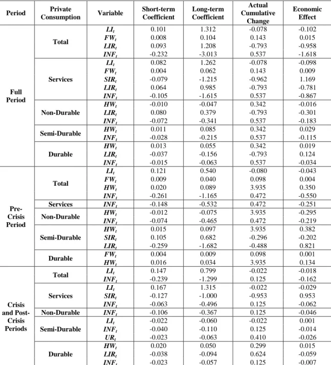
Finally, we present the economic significance of our statistically significant estimates (McCloskey and Ziliak, 1996; Ziliak and McCloskey, 2004) in order to correctly identify the drivers of private consumption and the role of financialisation on its evolution in the EU countries since 1995. Results are presented in Table 6.
Table 6 – Economic significance of our estimates for private consumption by durability Period Private Consumption Variable Short-term Coefficient Long-term Coefficient Actual Cumulative Change Economic Effect Full Period Total LIt 0.101 1.312 -0.078 -0.102 FWt 0.008 0.104 0.143 0.015 LIRt 0.093 1.208 -0.793 -0.958 INFt -0.232 -3.013 0.537 -1.618 Services LIt 0.082 1.262 -0.078 -0.098 FWt 0.004 0.062 0.143 0.009 SIRt -0.079 -1.215 -0.962 1.169 LIRt 0.064 0.985 -0.793 -0.781 INFt -0.105 -1.615 0.537 -0.867 Non-Durable HWt -0.010 -0.047 0.342 -0.016 LIRt 0.080 0.379 -0.793 -0.301 INFt -0.072 -0.341 0.537 -0.183 Semi-Durable HWt 0.011 0.085 0.342 0.029 INFt -0.028 -0.215 0.537 -0.115 Durable HWt 0.013 0.055 0.342 0.019 LIRt -0.037 -0.156 -0.793 0.124 INFt -0.015 -0.063 0.537 -0.034 Pre-Crisis Period Total LIt 0.121 0.540 -0.080 -0.043 FWt 0.009 0.040 0.098 0.004 HWt 0.020 0.089 3.935 0.350 INFt -0.261 -1.165 0.472 -0.550 Services INFt -0.148 -0.532 0.472 -0.251 Non-Durable HWt -0.012 -0.075 3.935 -0.295 INFt -0.074 -0.465 0.472 -0.219 Semi-Durable HWt 0.015 0.097 3.935 0.382 SIRt 0.105 0.682 -0.296 -0.202 LIRt -0.259 -1.682 -0.488 0.821 Durable FWt 0.004 0.009 0.098 0.001 HWt 0.016 0.034 3.935 0.134 Crisis and Post-Crisis Periods Total LIt 0.147 0.799 -0.022 -0.018 INFt -0.239 -1.299 0.125 -0.162 Services LIt 0.167 1.315 -0.022 -0.029 SIRt -0.127 -1.000 -0.953 0.953 INFt -0.063 -0.496 0.125 -0.062 Non-Durable INFt -0.106 -0.367 0.125 -0.046 Semi-Durable LIt -0.022 -0.060 -0.022 0.001 INFt -0.040 -0.110 0.125 -0.014 URt -0.023 -0.063 0.410 -0.026 Durable HWt 0.020 0.050 0.299 0.015 LIRt -0.038 -0.094 0.624 -0.059 INFt -0.023 -0.057 0.125 -0.007
Note: The long-term coefficient is obtained through the division between the short-term coefficient (estimated coefficient) and one minus the coefficient of the autoregressive estimation (estimated lagged consumption coefficient). The actual cumulative change corresponds to the growth rate of the correspondent variable. The economic effect is the multiplication of the long-term coefficient by the actual cumulative change
Taking into account the full period, we conclude that financial wealth was the single driver of total private consumption, whilst the inflation rate, the long-term interest rate and the labour income have the worst impact. Effectively, the increase of financial wealth favoured an acceleration of total private consumption by 1.5 per cent. However, the increase in inflation rate,
the decrease of long-term interest rates and the fall in labour income contributed to a decline in total private consumption by around 162, 96 and 10 per cent, respectively. Against this backdrop, the global net effect of financialisation on total private consumption was detrimental taking into account that the increase of households’ financial wealth was not sufficient to compensate for the fall in households’ labour income. This was transversal to all the components of total private consumption and even in the case of consumption of goods (non-durable, semi-durable and durable) because the growth of housing wealth was clearly insufficient to counterbalance the deleterious effects caused by the other variables.
Until the Great Recession, the increase of the inflation rate and the fall in labour income were also prejudicial to total private consumption. The total private consumption would have been higher by 55 and 4.3 per cent if there had not been a rise in the inflation rate and a decline in labour income, respectively. The increase of financial and housing wealth was both beneficial to total private consumption by delineating an acceleration of it by 0.4 and 35 per cent. The increase of housing wealth was in fact the main driver of total private consumption and of the consumption of both semi-durable and durable goods in the pre-crisis period. Accordingly, the global net effect of financialisation on total private consumption was strongly positive until the crisis, which was more evident in the case of consumption of semi-durable and durable goods.
During and after the crisis, the total private consumption was again negatively squeezed by the increase of the inflation rate and by the drop of labour income, which implied a deceleration of total private consumption by around 16 and 2 per cent, respectively. Thus, financialisation has had a harmful effect on the evolution of total private consumption in the EU countries since the emergence of the Great Recession, which is particularly due to the fall of labour income and more notorious in the case of consumption of services. The only exception is consumption of durable goods, where financialisation has a beneficial effect due to the rise of housing wealth.
Summing up, we confirm the two contradictory effects of financialisation on total private consumption (Stockhammer, 2009; Onaran et al., 2011; Hein, 2012) in the EU countries. It is true that the fall of labour income and the rise of both financial and housing wealth are general trends before, during and after the crisis, but the global net effect of financialisation differs across time. In the pre-crisis period, financialisation implied an acceleration of total private consumption because the wealth effect suppressed the income effect. This was more evident in the case of consumption of semi-durable and durable goods. In the crisis and post-crisis periods, financialisation implied a deceleration of total private consumption essentially because of the pronounced drop in households’ labour income. This was more notorious in the
case of consumption of services. Looking at the full period, financialisation had a detrimental effect on total private consumption and in all components because the wealth effect was not enough to counteract the income effect and/or the negative effect caused by the remaining variables.
6.2 DIFFERENT GROUPS OF SIMILAR COUNTRIES
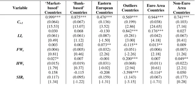
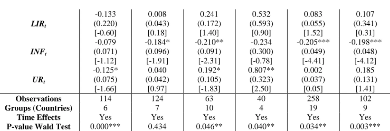
In this Subsection, we present the estimates of our private consumption equation by splitting our sample into different groups of similar countries. This approach allows for taking advantage of the cross-sectional dimension of our panel data and addresses whether private consumption has been influenced in the same manner and/or degree in the different EU countries, namely in terms of financial system and Euro area membership.7 For simplicity and in order to avoid dealing with quite small samples, this analysis only assesses total private consumption and the full period. Results are presented in Table 7.
Table 7 – Estimates of private consumption by different groups of countries for full period (1995-2015)
Variable ‘Market-based’ Countries ‘Bank-based’ Countries Eastern European Countries Outliers Countries Euro Area Countries Non-Euro Area Countries Ct-1 0.999*** (0.064) [15.53] 0.875*** (0.067) [13.07] 0.476*** (0.136) [3.52] 0.569*** (0.199) [2.86] 0.944*** (0.038) [24.65] 0.741*** (0.103) [7.16] LIt 0.030 (0.061) [0.49] 0.068 (0.061) [1.12] -0.130 (0.087) [-1.50] 0.842*** (0.281) [3.00] 0.176*** (0.042) [4.18] 0.027 (0.067) [0.41] FWt 0.003 (0.004) [0.81] 0.002 (0.005) [0.46] 0.073** (0.032) [2.26] -0.115** (0.051) [-2.26] 0.013** (0.006) [2.18] 0.009 (0.007) [1.26] HWt 0.027* (0.015) [1.79] 0.007 (0.019) [0.37] -0.001 (0.031) [-0.02] 0.200*** (0.068) [2.94] 0.007 (0.011) [0.61] 0.049** (0.022) [2.21] SIRt 0.158 (0.117) [1.34] -0.115 (0.095) [-1.22] -0.208 (0.159) [-1.31] -3.598*** (1.143) [-3.15] -0.114* (0.067) [-1.71] 0.050 (0.177) [0.28]
7 According to Bijlsman and Zwart (2013) and Haan et al. (2015), the EU countries are clustering in four
different groups following the characteristics of their financial systems. The first group is the ‘market-based’ countries, including Belgium, Finland, France, the Netherlands, Sweden and the United Kingdom. These countries have a financial system quite similar to the one of the USA. The second group is the ‘bank-based’ countries, which includes Austria, Denmark, Germany, Greece, Italy, Portugal and Spain. These countries more closely resemble Japan due to the strong importance of banks in their financial systems. The third group is the eastern European countries, which includes Bulgaria, Czech Republic, Estonia, Hungary, Latvia, Lithuania, Poland, Romania, Slovakia and Slovenia. Some of these countries were recently incorporated into the Euro area and the majority have generally small financial systems. The fourth group is the outlier countries, including Cyprus, Ireland, Luxembourg and Malta. These countries have banking sectors that are both very large and extend a large amount of credit compared to their national economies. The group of Euro area countries includes Austria, Belgium, Cyprus, Estonia, Finland, France, Germany, Greece, Ireland, Italy, Latvia, Lithuania, Luxembourg, Malta, the Netherlands, Portugal, Slovakia, Slovenia and Spain. The group of non-Euro area countries includes the remaining countries.
LIRt -0.133 (0.220) [-0.60] 0.008 (0.043) [0.18] 0.241 (0.172) [1.40] 0.532 (0.593) [0.90] 0.083 (0.055) [1.52] 0.107 (0.341) [0.31] INFt -0.079 (0.071) [-1.12] -0.184* (0.096) [-1.91] -0.210** (0.091) [-2.31] -0.234 (0.300) [-0.78] -0.205*** (0.049) [-4.41] -0.198*** (0.048) [-4.12] URt -0.125* (0.075) [-1.66] 0.040 (0.042) [0.97] 0.192* (0.105) [-1.83] 0.807** (0.323) [2.50] 0.002 (0.037) [0.05] 0.185 (0.131) [1.41] Observations 114 124 63 40 258 102 Groups (Countries) 6 7 10 4 19 9
Time Effects Yes Yes Yes Yes Yes Yes
P-value Wald Test 0.000*** 0.434 0.046** 0.040** 0.034** 0.003***
Note: Standard errors in ( ), z-statistics in [], *** indicates statistical significance at 1% level, ** indicates statistical significance at 5% level and * indicates statistical significance at 10% level. Coefficients, standard errors and z-statistics for the year dummies are not reported
Note first that the sluggishness of total private consumption and the negative effect of the inflation rate are confirmed for the majority of country groups. The results for the remaining variables differ slightly between the six groups of countries. For the ‘market-based’ countries, housing wealth remains statistically significant by positively influencing private consumption, whilst the unemployment rate comes up as a negative determinant. In the case of the eastern European countries, the inflation rate maintains its negative influence on private consumption, whilst financial wealth and unemployment rate become statistically significant by exerting a positive effect. The most counterintuitive result concerns unemployment rate by suggesting that an increase in the unemployment rate implies an acceleration of total private consumption, which can be attributed to the existence of unemployment benefits that function as automatic stabilisers, the utilisation of savings, and rising debt by households. This happens due to the aforementioned ‘ratchet effect’ (Duesenberry, 1949). In relation to the outlier countries, labour income, housing wealth and unemployment rate exert a positive influence on total private consumption, whilst the short-term interest rate emerges as a negative driver.
With regard to Euro area membership, results differ slightly between the two groups of countries. The results for the Euro area countries are quite similar to the results obtained for all countries in terms of statistical significance and signs. The only exception pertains to the short-term interest rate that becomes statistically significant in the case of the Euro area countries, by negatively influencing total private consumption. Results for the non-Euro area countries show that housing wealth is a positive determinant of total private consumption.
Table 8 contains the economic significance of our statistically significant estimates (McCloskey and Ziliak, 1996; Ziliak and McCloskey, 2004) for the different groups of countries in order to assess the drivers of private consumption on its evolution in each group since 1995.