Finite state machine modelling of the macro-economy

Finite State Machine Modelling of the

Macro-Economy

João Marques Silva and José Azevedo Pereira

Email: joao.silva@iscte.pt; jpereira@iseg.ulisboa.pt

Abstract—In this paper we model macro-economic policies

with a Finite State Machine (FSM). The FSM is made of several states and transitions between states, in which a state is modelled by a set of conditions. The allowed transitions between states must be also be defined, in order to complete the model. In this paper we analyze how to use a FSM in order to model macroeconomic decision, where each state represents a set of economic decisions. Together with some pre-defined initial conditions, these adapted FSM models are analyzed in order for us to study what sequence of decisions yield the best results for pre-determined end-goals, based on the FSM’s possibilities. The final model shows what policies must be followed, and by what order, in order to maximize results, yielding some interesting conclusions.

Index Terms—finite state machines, macro economy,

modelling, politics1

I. INTRODUCTION

Economic models are complex, since a country’s economy is dependent on politics, people’s reactions to politics, resource limitations, environmental and geographical constraints, institutional and legal requirements, other countries’ interactions, etc. Put it simply, a country’s economy is dependent on so many aspects that makes it very hard to predict.

Since the classical model (that focused on the equilibrium between supply and demand for labor) [1] in 1776, we focused on the Keynesian Models (1936-1969), that started as a vastly oversimplified view of the economy, constructing an equilibrium without referring to the labor market, showing that an economy can be in equilibrium without having full employment [2-3]. The Keynesian model is then expanded to the IS / LM (Interest Saving – Liquidity Money Supply) model, focusing on long-term and short-term interest rates. Income and the interest rate are variables used to achieve equilibrium. The model was updated from a closed to an open economy with the Balance of Payments (BoP) in the Mundell-Fleming model (also known as IS-LM BoP model) [4-5]. In 1970 a “new” classical model was introduced, shifting attention from nominal interest rates back to the real factores of production that dominated the original classical model [6-7]. After the recession in 1982, the

Manuscript received June 18, 2017; revised August 31, 2017

debate about the real effects of nominal monetary policy was reopened, and the IS/MP (Monetary Policy) model was created [8], addressing a perceived shortcoming of the IS-LM model, replacing the price level with the inflation rate and by replacing the nominal interest rate with the real interest rate.

More recently, some new economics models have come into play [9-10], but all differ from each other and have different purposes. In this paper, we devised a simple model, based on Finite State Machines (FSM). This form of representation is disruptive on economic models, and focuses on the economy’s evolution based on a pre-determined set of (political) decisions, and is used to determine which set of decisions must be taken in order to maximize a chosen variable (Gross Domestic Product, for example).

The paper is structured as follows: in section II we introduce Finite State Machines and in section III we build a macroeconomic model based on Finite State Machines. Section IV portrays some results that stem from different transitions (decisions) in the model, and in section V some conclusions are drawn.

II. FINITE STATE MACHINES

A Finite-State Machine (FSM) is a mathematical model used to represent different states and the transitions between them. The theory of FSM is explained in [11], and stemmed from work in [12], with the original presentation of regular expressions and their connection with machines. Particularization of the machines with output that were a function of state and input [13] and a function of solely the state [14] were drawn by G.H. Mealy (Mealy Machines) and Edward F. Moore (Moore Machines) respectively.

In this paper we make use of Mealy machines (outputs dependent on both state and input) and model macro-economic policies by different states, studying the effect of different sets of transitions between them. The policies can be user-defined, and the number of states is unlimited, though for simplicity and clarity we suggest a maximum of 4. This model will serve as a basis for studying the best transitions between states to obtain certain macro-economic results, and to predict the economy’s evolution in future works.

III. ECONOMIC MODEL BASED ON FSM A 4-state machine was devised, where each state represents one of four different kinds of political decisions. The variables that were selected to model each state can be changed; however, the used values were chosen to serve as a practical (and somewhat realistic) example. With the FSM mechanism, we can model a country’s economy (or any economy, for that matter) by a stochastic process, and use it to forecast economic activity and/or propose changes in economic policies.

This model provides an argumentative framework that can be discussed and tested for different scenarios. Since it is a simple representation of the complexities of the economy, its results will serve as approximate representations of the economy, highlighting key relationships between some variables.

The model must be adjusted for accuracy by cross-checking with historical data and fine-tuning the characteristics of each state. This should be an iterative process until all states are good representations of the reality. The used aggregate variables can be modified and validated by econometrics. The model is built to sustain deterministic chaos, caused by sudden change in policies and portrayed by certain transitions between states. Future works can portray those changes by probabilities linked to state transitions.

The policies of each state will influence its variables, which are the same for all states. The influences will reference overall variables that we defined as (these values were used as an example; they can be changed):

Z (Discount rate) 3%

Tax level 75%

UF (Unfairness Factor) 10

Number of workers 600

The model that was used as an example is portrayed in Fig.1:

Figure 1. 4 state FSM model with all possible transitions Each of the four states represents certain policies, with the corresponding variables change. We assume that once a transition has been made, things will evolve according to the state’s variable functions during one period. Since the states are connected in a full-mesh, any state can evolve to any other state, including itself. The state’s policies are as follows (depicted in Table I):

After each transition, the state’s variables are updated. Once changed, the variables they are assumed fixed throughout the whole period (year, in this case), and used

for the “throughout the year calculations” of the following variables:

Expenses = Expense coefficient x Total money Tax = Tax level*(40% total money + 60% mean wages x number workers x (1- unemployment)) x (1 - Tax evasion)

Debt Interest= Z times debt

Cost each unit = Total money / Production Yearly Profit = Taxes collected - Expenses - Debt interest

Political value = 5*Mean Wage/ Cost per Unit + 1/(10 x Unemployment)

Economic value =Production * (Political Value/2 + (Exports/Imports) + expected(Taxes collected/Expenses)-Debt/Total money+1/(Debt spread*10))

TABLEI.DEFINING CONDITIONS OF EACH STATE

Note that both the political and economic value are values only useful for simulation purposes. Some memory effect will be considered for the “economic progress” state (scenario A), in which remaining in such state for after 3 periods will have a different effect in its defining variables. Such is the case for Scenario A. namely for the expense coefficient and unemployment. It is assumed that the first 3 consecutive times each value will decrease (Z% and 1% respectively), and will then either rise or stay constant after the fourth consecutive year. The authors decided that scenario A wouldn’t remain perfect ad eternum, and thus admitted that expenses would break loose at the 4th consecutive year (election effect), while unemployment would stop descending.

Scenario B assumes that the government will “print money” to pay off the whole of its debt, and suffer some consequences with the debt spread and tax evasion. It also introduces the notion of “fair wage”, which basically is equal to the proportion of total money increase; Fair wage = initial wage x (new total money/ total money previous year), which means that the fair wage wouldn’t render any loss in buying power.

Scenario C assumes that the policies for the current year will center on the repositioning of just wages (re-instate the same purchasing power as in the initial state), causing a positive effect on tax evasion, but increasing

Scenario A - no debt payment

Scenario B - with total debt payment Scenario C - repositioning of just wages Scenario D - Austerity measures Boundaries Total money + Z%

total money plus

debt = = >0 Production + Z% = = - 2Z >0 Mean wage + Z% Decreases UFxZ compared to fair wage Total money x 60% / number workers - 2Z >0 Expense coefficient - Z% for 3x in a row, then +2Z = = - 4Z (min,max 20%,90%) Tax evasion = +25% -10% +10% (min,max 5%,90%) Unemployment -1% for 3x in a row, then = - 3% + 5% + 2% (min,max 2%,50%) Debt spread -1% + 15% + 3% - 2Z (min,max 1%,30%) Imports = -UFxZ Increases by

wage increase % - 2Z (min 0)

Exports = + +/= + (min 0)

Exchange Rate =

Devaluation of

both the unemployment rate and debt spread. Scenario D, on the other hand, assumes a scenario of austerity, which reduces the expense coefficient and debt spread, but has negative effects on the economy.

The exports of each state are calculated from the following formulas:

IV. RESULTS

TABLEII.INITIAL CONDITIONS FOR SIMULATOR

Variable Value units Goal

Total money 1 000 000

currency maximize Production 1 000 units maximize Mean wage 1 000 currency maximize

Debt 1 000

000

currency minimize Expense coefficient 40% minimize

Tax evasion 15% minimize

Unemployment 12% minimize

Debt spread 1% minimize

Imports 100 units minimize

Exports 100 units maximize

Exchange Rate 1 domestic/fore ign

maximize With all the rules explained, we are now in the condition of running the model. A simulator was built, that runs all possible combinations of the model for a number of iterations (each iterations represents a year). Having all results from all possible combinations, we can assess which state transitions yield the best values (maximum or minimum, depending on the case) for each variable. Note that we don’t deal with transition

probabilities (yet), rather we will just study what transitional sequences lead to specific results, and analyse those transitions.

Starting with the initial conditions depicted in Table I, where the goal for each variable is detailed:

We can run the simulator for all combinations in order to obtain the best transition sequences for all iterations (in this case, years); this in portrayed in Table III. Looking at the table, we can see that the sequences can suffer some changes between years, meaning that the best transition sequence to maximize/minimize a variable on year x might be significantly different than for year x+1. Looking at the case of Debt (here, the smaller the Debt, the better; negative debt represents a surplus), we have that while the best transition sequence for 3 years is 112 (representing a transition to state 1 for the first and second year, and a transition to state 2 at the third year), the best transition to minimize debt for 4 years is totally different (4321) – one could expect that the transitions for the first 3 years would remain the same (112), but this proves it different.

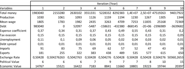
In Table IV, we have the yearly evolution of the values for the best transition state of 10 years (the rightmost column of Table III). Looking at the debt for reference again, we can see that the transition for year=2 was 2, which means cancelling off the debt (and thus the debt value for that value is 0). The value evolves to a negative value (meaning that our country has loaned money to someone else and is getting interest on it). Some values of interest for governments would be the political value and/or the economic value; each of these values have different transition sequences to maximize them, and it is interesting to see that, according to our model, both value rise and fall across the years in order to obtain their highest value in year 10. This simple model thus summarises one big economic and universal truth; sometimes we need to take some steps back in order to move forward. Since in politics we have waves of 4-5 years mandates, we can see by this examples that governments would only be interested in taking actions to maximize some variables on a shorter term.

TABLEIII. BEST TRANSITION SEQUENCES FOR EACH VARIABLE, ACCORDING TO NUMBER OF ITERATIONS (YEARS)

Variables 1 2 3 4 5 6 7 8 9 10 Total money 2 22 222 2222 22222 222222 2222222 22222222 222222222 2222222222 Production 1 11 111 1111 11111 111111 1111111 11111111 111111111 1111111111 Mean wage 2 23 223 2232 22232 222232 2222232 22222232 222222232 2222222232 Debt 2 12 112 4321 43231 432331 4323331 43233311 432333131 4233331311 Expense coefficient 4 44 144 1114 11124 111144 1111144 11111244 111111444 1111111444 Tax evasion 3 13 113 1113 11113 111113 1111113 11111113 111111113 1111111113 Unemployment 2 22 222 2221 11222 122111 1121211 11221111 112211111 1112124111 Debt spread 1 11 111 1111 11111 111111 1111111 11111111 111111111 1111111111 Imports 2 22 222 2222 22222 222222 2222222 22222222 222222222 2222222222 Exports 4 44 444 4242 22222 222222 2222222 22222222 222222222 2222222222 Exchange Rate 1 11 111 1111 11111 111111 4323332 43233332 412133332 2433133412 Political Value 1 11 222 1222 11222 111212 1112121 11112121 111112121 1122231211 Economic Value 1 11 111 1111 14111 114111 1113111 11131111 111311111 1113111111 Iteration (Year)

Exports = Production - National consumption National consumption = Total consumption - imports Total consumption = Production x (Mean Wage/ Cost of each unit)

Our model can be changed both in the initial conditions, number of states, state rules and possibilities of transitions. So being, another simulation was run, but this time we

disallowed recursion on states 2 and 3; meaning that when on state 2 or state 3, we can’t have a transition to the same state on the following year (Fig. 2).

TABLEIV.YEARLY EVOLUTION OF EACH VARIABLE, FOR THE BEST TRANSITION STATE OF 10YEARS

Figure 2. 4 state FSM model with some transition restrictions

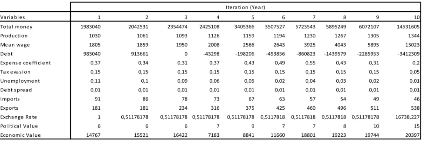
With this restriction, we obtained the new tables, Table V and Table VI, with significantly different transitions, and, as expected, some final values that were either the same or a bit worse (higher or lower casuistically). Looking at the political value as an example, we see that the final value is still 15, with transitions moving from (1122231211) to (2121231211), which is substantially different, but yielding a similar result. A well-tuned model could help governors decide on their strategy according to existing constraints, and have a means of communicating the message and set their objectives.

The results for the FSM model without recursion on states 2 and 3 are as follows (portrayed in Table V and Table VI):

TABLEV.BEST TRANSITION SEQUENCES FOR EACH VARIABLE, ACCORDING TO NUMBER OF ITERATIONS (YEARS), WITHOUT RECURSION ON STATES 2 AND 3

Variables 1 2 3 4 5 6 7 8 9 10

Total money 1983040 2153280 2630102 3551331 5228332 8292383 1,4E+07 2,5E+07 47519263 94017922

Production 1030 1061 1093 1126 1159 1194 1230 1267 1305 1344 Mean wage 1805 1783 1982 2435 3263 4709 7253 11835 25168 72369 Debt 983040 0 52097 -5487 -158631 -432380 -868145 -2E+06 -2396989 -3639682 Expense coefficient 0,37 0,34 0,31 0,37 0,43 0,49 0,55 0,43 0,31 0,2 Tax evasion 0,15 0,15 0,15 0,15 0,15 0,15 0,15 0,15 0,15 0,05 Unemployment 0,11 0,1 0,09 0,06 0,05 0,02 0,04 0,03 0,02 0,01 Debt spread 0,01 0,01 0,01 0,01 0,01 0,01 0,01 0,01 0,01 0,01 Imports 91 83 75 69 62 57 52 47 43 39 Exports 181 255 322 383 438 489 535 577 615 650 Exchange Rate 0,50428 0,504276263 0,5042763 0,50428 0,504276 0,50428 0,50428 0,50428 0,504276 50360,2653 Political Value 6 6 6 7 9 7 7 8 10 15 Economic Value 14767 15521 16422 7183 8841 11660 18801 19223 19744 20397 Iteration (Year) Variables 1 2 3 4 5 6 7 8 9 10 Total money 2 21 212 2112 21212 212112 2121212 21212112 212121212 2121212112 Production 1 11 111 1111 11111 111111 1111111 11111111 111111111 1111111111 Mean wage 2 23 232 2123 21232 212132 2121232 21212132 212121232 2121212132 Debt 2 12 112 4321 43231 432311 4323131 43231311 432313131 4323131311 Expense coefficient 4 44 144 1114 11124 111144 1111144 11111244 111111444 1111111444 Tax evasion 3 13 113 1113 11113 111113 1111113 11111113 111111113 1111111113 Unemployment 2 12 212 2121 21212 212111 1121211 12121111 121211111 1112124111 Debt spread 1 11 111 1111 11111 111111 1111111 11111111 111111111 1111111111 Imports 2 24 242 2424 24242 242424 2424242 24242442 242424242 2424242424 Exports 4 44 444 4242 24242 244242 2424242 42424242 242424242 2124244242 Exchange Rate 1 11 111 1111 11111 111111 4311132 43231312 413231312 3213134342 Political Value 1 11 111 1212 21212 111212 1112121 11112121 111112121 2121231211 Economic Value 1 11 111 1111 14111 114111 1113111 11131111 111311111 1113111111 Iteration (Year)

TABLEVI. YEARLY EVOLUTION OF EACH VARIABLE, FOR THE BEST TRANSITION STATE OF 10YEARS, WITHOUT RECURSION ON STATES 2 AND 3

V. CONCLUSION

This work modelled different economic evolutions due to different political decisions, supported by the application of a Finite State Machines (FSM). In fact, political decisions are focused on maintaining popularity first, and insuring high economic value second. We demonstrated that the economy’s evolution may not always follow the best long-term result, being merely centered on periodic election cycles – this being, the key question that society must place as a whole is how to ensure that economic plans are made on the long-term while maintaining the democratic degree of freedom – this or a similar tool must be used by future decision-makers in order to ensure the best long-term decisions and results. In future works, a Markov mode (a stochastic model used to model randomly changing systems where it is assumed that future states depend only on the current state not on the events that occurred before it) will be assumed in order to account for uncertainty.

ACKNOWLEDGE

We gratefully acknowledge financial support from FCT- Fundação para a Ciencia e Tecnologia (Portugal), national funding through research grant (UID/SOC/04521/2013).

REFERENCES

[1] S.Adam,An Inquiry into the Nature and Causes of the Wealth of Nations,1(1 ed.). London: W. Strahan. 1776.

[2] J. M. Keynes, The General Theory of Employment, Interest and

Money, Macmillan Cambridge University Press, for Royal

Economic Society, 1936.

[3] R. J. Hicks, Mr. Keynes and the “Classics”; a suggested

interpretation, Econometria, vol. 5, pp. 147-159, 1937.

[4] A. M. Robert, “Capital mobility and stabilization policy under fixed and flexible exchange rates," Canadian Journal of Economic

and Political Science, vol. 29, no. 4, pp. 475–485.

[5] J.F.Marcus,“Domestic financial policies under fixed and floating exchange rates,"IMF Staff Papers,vol. 9, pp.369–379.

[6] M. Friedman, The Counter-Revolution in Monetary Theory, Institute of Economic Affairs, London, 1970.

[7] J. R. Barro, “Second thoughts on keynesian economics,”American Economic Review, Proceedings. May, 1979.

[8] R. David, “Keynesian macroeconomics without the LM curve,”Journal of Economic Perspectives,vol. 14, no. 2, pp. 149-169, 2000.

[9] K. Lawrence, “The contribution of Jan Tinbergen to economic science,”De Economist, vol. 152, no. 2, pp. 155–157, 2004.

[10] R. K. Narayana, “Model fit and model selection,”Federal Reserve Bank of St. Louis Review, vol. 89, pp. 349–60, 2007.

[11] A. Gill, Introduction to the Theory of Finite-state Machines. McGraw-Hill, 1962.

[12] S. C. Kleene, “Representation of events in nerve nets and finite automata,” Shannon and McCarthy (eds.), Automata Studies,

Annals of Mathematics Studies, Princeton University Press, no. 34,

pp. 3-41, 1956.

[13] G. H. Mealy, “A method for synthesizing sequential circuits,”The Bell System Technical Journal, vol. 34, no. 5, pp. 1045-1079,

September 1955.

[14] F. E. Moore, “Gedanken-experiments on sequential machines,” in Shannon and McCarthy (eds.), Automata Studies, Annals of

Mathematics Studies, Princeton University Press, no. 34, pp

129-153, 1956.

João Carlos. M. Silva received the BSc and MSc degree for Aerospace Engineering from Instituto Superior Técnico (IST) – Lisbon Technical University, (1995-2000). From 2000-2002 he worked as a business consultant in strategic management in McKinsey&Company. From 2002 to 2006 he undertook his PhD in telecommunications at IST, integrated in 3 EU projects (Seacorn, B-Bone e C-Mobile), having been the representative of the university. Since 2006, he has been working on computer networks, as an assistant professor in Instituto Superior das Ciências do Trabalho e da Empresa (ISCTE). Recently, he finished his MBA at ISEG (Instituto Superior de Economia e Gestão), and aims to work on technological management in the near future. Email: joao.silva@iscte.pt

José Azevedo Pereira is a full Professor of Finance, at Universidade de Lisboa, ISEG - Instituto Superior de Economia e Gestão. He holds a PhD from the Manchester Business School and an MBA, from ISEG. Besides his academic career he has held top executive positions in several companies. During seven years he led the Portuguese Tax and Customs Authority, where he was Director-General and Chairman of the Board. Email: jpereira@iseg.utl.pt Va ri a bl es 1 2 3 4 5 6 7 8 9 10 Tota l money 1983040 2042531 2354474 2425108 3405366 3507527 5723543 5895249 6072107 14531605 Producti on 1030 1061 1093 1126 1159 1194 1230 1267 1305 1344 Mea n wa ge 1805 1859 1950 2008 2566 2643 3925 4043 5895 13023 Debt 983040 913661 0 -43298 -198206 -453856 -860823 -1439579 -2285953 -3412309

Expens e coeffi ci ent 0,37 0,34 0,31 0,37 0,43 0,49 0,55 0,43 0,31 0,2

Ta x eva s i on 0,15 0,15 0,15 0,15 0,15 0,15 0,15 0,15 0,15 0,05 Unempl oyment 0,11 0,1 0,09 0,06 0,05 0,02 0,04 0,03 0,02 0,01 Debt s prea d 0,01 0,01 0,01 0,01 0,01 0,01 0,01 0,01 0,01 0,01 Imports 91 86 78 73 67 63 57 54 49 46 Exports 181 181 234 316 375 425 460 496 511 538 Excha nge Ra te 1 0,51178178 0,51178178 0,51178178 0,51178178 0,5117818 0,5117818 0,5117818 0,51178178 16738,227 Pol i ti ca l Va l ue 6 6 6 7 9 7 7 8 10 15 Economi c Va l ue 14767 15521 16422 7183 8841 11660 18801 19223 19744 20397 Itera ti on (Yea r)