On the effects of bilateral investment treaties on foreign domestic investment: Why not all directions?
Lucas P. do C. Ferraz1 Marcel B. Ribeiro2
1.
Introduction
Bilateral investment treaties (BITs afterward) have become a popular tool among policymakers with the purpose of promoting and protecting foreign investment. Formally, BITs establish terms and conditions for private investment from one country (or a country group) into another. Specifically, they regulate issues such as admission and establishment of investment, fair and equitable treatment according to international law, expropriation, and the settlement of disputes at the bilateral level. Setting the rules of the game before investments are undertaken, ensure a more transparent and stable investment environment that diminishes risks for investors. Ultimately, these regulations should lead to greater foreign direct investment (FDI afterward) among the treaty members.
Figure 1 shows the increase of adoption of new BITs for the period of 1962 to 2017. The years are from the date of entry in force, that is, the date in which the agreement becomes binding. During the 1960s until the mid-1980s there was a small and steady adoption of new BITs. During the 1990s and early 2000s, there was a sharp acceleration of the BITs getting in force whereas a deceleration can be noticed afterward. According to UNCTAD (2006), after the mid-1990s there was also a substantial change regarding the content of the treaties by including investment protection provisions and investor-State dispute settlement provisions.
1 Sao Paulo School of Economics (Getulio Vargas Foundation). 2 Sao Paulo School of Economics (Getulio Vargas Foundation).
Figure 1. Evolution of new bilateral investment treaties through time by development groups
Source: UNCTAD’s international investment agreement database. Authors calculations.
Figure 1 also distinguishes the BITs by the development level of members. The dynamics of the BIT adoption is similar among groups, but is clear that the majority of BITs are signed between developed and developing countries (roughly 58%). However, an important share of the treaties is between developing countries (roughly 35%). Agreements including least developed countries (LDC afterward) and among developed countries only exists, but they are a minority (approximately 6.5%).
In this report, we evaluate the role of BITs on FDI by estimating a gravity equation for foreign investment flows. Unlike previous studies, we assess the effects of BITs for all countries groups. Most of the literature focuses on the relationship of developing countries being
0 50 100 150 200 250 300 350 400 19 62 19 64 19 66 19 68 19 71 19 73 19 75 19 77 19 79 19 81 19 83 19 85 19 87 19 89 19 91 19 93 19 95 19 97 19 99 20 01 20 03 20 05 20 07 20 09 20 11 20 13 20 15 20 17
the destination of the foreign investment from developed countries. Instead, we evaluate the effects of BITs including least developed, developing and developed countries as both origin and destination on the FDI of those countries.
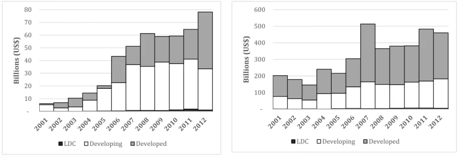
Figure 2 shows the evolution of FDI during the 2000s of FDI from developing (panel (a)) and developed countries (panel (b)) into each development group destination. We do not include FDI originated from LDC because it accounts for less than 1% of total FDI. By comparing the scale of panels, one can see that developed countries invest abroad roughly eight times more than developing countries. In 2001, the investment in developed countries accounted for around 96% of total FDI, but it decreased steadily to about 85% in 2012. This drop in share is a result of the substantial increase in FDI from developing countries, in particular, after 2005.
Moreover, panel (b) of Figure 2 the flow of investment from developed countries to developing is about U$100-150 billion, which is only roughly 38% of total foreign investment of developed countries and 34% of total FDI. Therefore, when focusing on the relationship of developing as hosts and developed countries as origin, the literature does not take into account 66% of total FDI (55% between developed countries and 10% originating from developing countries and 1% originating from LDCs) and 42% of all BITs in force (35% between developing countries and 6.5% of other relationships).
Most of the studies use the OLS estimator to estimate the impact of BITs on the FDI, with the notable exception of Desbordes and Vicard (2009). As in the latter, we contribute to the literature estimating the gravity model for FDI using the PPML estimator. As shown by Santos Silva and Tenreyro (2006), the Poisson pseudo maximum likelihood estimator (PPML) corrects for biased estimates due to heteroscedasticity for log-linear models. Another advantage of the PPML estimator is that it allows to use information from zero FDI flows, which is not possible with OLS because the dependent variable is the log of FDI. Additionally, we explore the differences in the estimates with the full sample and excluding the zeros to evaluate if there is a difference in the effect of BITs on the intensive and extensive margin of investment decisions.
Figure 2. Evolution of FDI flows by country destination
(a) Developing countries (b) Developed countries
Source: UNCTAD’s bilateral foreign direct investment database. Authors calculations.
Our primary results are the following. First, we found weak evidence of positive the effects of BITs, if any. For the standard specifications in the literature, we found positive and significant effects at 10% of significance. Whenever controlling for fixed effects and/or multilateral resistance, the significance of the impact of BITs vanish. This is true for all country groups considered: least developed, developing and developed countries. Actually, evidence of a positive effect of BITs is slightly stronger for developed countries as hosts. We rationalize that the differences in our results from the main findings in the literature are owing to two factors. First, we show when using robust standard errors – the standard approach in this literature – the impact of BIT is positive and statistically significant at 1%. When using clustered standard errors by country-pair, which we consider more appropriated because of the data
10 20 30 40 50 60 70 80 Bil lio ns (US $) LDC Developing Developed 100 200 300 400 500 600 Bil lio ns (US $) LDC Developing Developed
structure, the significance vanishes as the estimated standard errors increase owing to the correlation in the regressors in this particular dimension. Second, when controlling for multilateral resistance, the impact of BIT becomes insignificant even when using robust standard errors. The multilateral resistance fixed effects are the standard approach in the trade literature and are consistent with the theoretical foundation for FDI flows of Head and Ries (2008).
We also contribute to the discussion on the interactions between BITs and domestic institutions. Two competing interpretations are advocated in the literature. First, Neumayer and Spess (2005) discuss that by signing BITs, countries indicate the willingness to provide further reassurance of property rights protection that is not guaranteed by domestic institutions. Under such a hypothesis, a BIT acts as a substitute to improvements in institutional quality. Alternatively, the implementation of a BIT can be viewed as further signaling that the property rights established domestically are also applied to foreign investment in detriment of eventual national goals. In the latter case, BITs and good domestic institutions are then complementary as discussed by Hallward-Driemeier (2003).
Although we do not find robust evidence on the unconditional effect of BITs on FDI, we find some interesting results by allowing the effects of BITs to vary according with the institutional quality of the investment destination country. Our results are robust regarding the substitutability of BITs and institutional quality for all country groups. However, which intuitional measure plays a more critical role depends on the country level of development. Our estimates suggest that BITs have a stronger impact on LDC with low political stability while such measure does not play an important role for developing and developed countries. On the other hand, we find a more pronounced impact of BITs for developing and developed countries with poor measures of control of corruption, whereas it does not play a role for LDC. This findings suggest that investors might have different layers of concerns regarding political risks in countries depending on their development level, and BITs can reassure investors regarding those layers.
2.
Data and Empirical analysis
Our sample consists of bilateral flows of FDI (in current dollars) are obtained from UNCTAD’s Bilateral FDI Statistics. The data includes 197 countries as both the origin and destination of the annual foreign direct investment flow for the period from 2006 to 2013. GDP and population data and political variables such as control of corruption and political stability are obtained from the World Bank. Standard gravity control variables, such as bilateral distance, common language, border sharing, and colonization are from the CEPII. From the same source, we also obtain data on free trade agreements and membership of WTO and OECD. Our variable of interest is a dummy, which is equal to one whenever a bilateral investment treaty is in force between the country pair. The BIT data is from the UNCTAD’s international investment agreement database.
The empirical analysis is based on the gravity equation, which is the workhorse model for bilateral trade flows. That model has been increasingly used to explain foreign direct investment flows (Wei, 2000; Carr et. al, 2001; Razin, and Sadka, 2007; Head and Ries, 2008 and many others). The gravity equation has a theoretical foundation for the bilateral trade follows (see Anderson and van Wincoop, 2003). More recently, Head and Ries (2008) and Bergstrand and Egger (2008) provided a theoretical foundation to the gravity equation for bilateral FDI.
The gravity specification used to estimate the impacts of NTBs on bilateral trade flows is described by equation (1):
𝐹𝑖𝑗𝑡 = exp(β𝐵𝐼𝑇𝑖𝑗𝑡+ 𝑿𝑖𝑗𝑡𝜃 + 𝛼𝑖+ 𝛾𝑗+ 𝜂𝑡) + 𝜀𝑖𝑗𝑠𝑡 (1)
where 𝑖 denotes the origin country, 𝑗 for the destination country, and 𝑡 for the time period. 𝐹𝑖𝑗𝑡 denotes the country 𝑖’s foreign direct investment flow into country 𝑗 at period 𝑡. The vector 𝑿𝑖𝑗𝑠𝑡 includes the standard gravity control variables: log of GDP and log of
population (for both destination and origin), distance, common language, border sharing and colonization. Those variables can control for the market size of both destination and origin countries as well costs involved in starting a business abroad or reinvesting into an existing one. We also include as explanatory variables two political variables: control of corruption and political stability indexes for both destination and origin countries (both are standardized).3 Those can help to control for perceived risk in the host and source countries, which can affect the likelihood of investors to get back the return of their investment.
The dummy variable 𝐵𝐼𝑇𝑖𝑗𝑡 is equal to one if countries 𝑖 and 𝑗 have at least one bilateral trade treaty in force at year 𝑡 and zero otherwise. Moreover, we include controls regarding the trade openness between the country pairs: whether there are trade agreements between them, whether they are both members of the OECD and they are members of the WTO. 𝛼𝑖, 𝛾𝑗 and 𝜂𝑡 denote the origin, destination and year fixed effects, respectively. In additional specifications, we use country pair, destination-year and origin-year fixed effects.
Following Santos Silva and Tenreyro (2006), we estimate equation (1) using the Poisson pseudo maximum likelihood estimator (PPML) since it corrects for biased estimates owing to the combination of the log transformation and presence of heteroscedasticity in the data. Moreover, the PPML estimator allows including FDI flows that are zero, i.e., we can use the information from countries that did not invest in each other to control for the ones who did. We also compare the results of the PPML including and not including the zero flows in the sample to evaluate if the effects of the BIT are through the intensive or extensive margin. Whenever using the OLS estimator, we take the log of equation (1) and estimate the standard log-log specification.
3 We also tests several specifications including other political variables available at the World Bank’s WGI. In those specifications, we included measures of control of corruption, political stability, regulatory quality, governance effectiveness, rule of law, and voice and accountability. In the specifications that we show in the text, we included the only the political variables that were statistically significant, namely, control of corruption and political stability.
2.1. Empirical Results
Table 1 shows the estimation of equation (1) via OLS, PPML, and PPML for the sample without zeros. Within each estimator, we control for different sets of fixed effects. The standard fixed effects used are origin, destination and year fixed effects, but we also test for country-pair and origin-year and destination-year fixed effects. As discussed by Baier and Bergstrand (2007) the country-pair fixed effects can alleviate the bias in estimation induced by the selection of free trade agreements. We use the same reasoning for BITs as it encompasses a similar political decision. In other words, the choice of a bilateral investment treaty is not random and might depend on the same characteristics that explain FDI. Such fixed effects to control for the decision of signing the BIT in the first place. Moreover, the origin-year and destination-year fixed effects in the trade literature controls for the so-called “multilateral resistance” (See, for instance, Anderson and van Wincoop, 2003; Feenstra, 2004), which also play a role in the context of investment decisions (Head and Ries, 2008).
The gradual inclusion of the fixed effects aforementioned is shown in columns (1-4) for the OLS, (5-8) for the PPML, and (9-12) for the PPML for positive FDI flows, respectively. Table 1 reveals several interesting points. First, there are important differences in the estimated coefficients depending on the estimator, which suggest a bias in the OLS estimation owing to a combination of log-linear transformation and heteroscedasticity (see Santos Silva and Tenreyro, 2006). When using the PPML estimator – an unlike the OLS estimation – coefficients are positive for control of corruption of the destination for all specifications (columns 5-6 and 9-10) and political stability of the destination using the full sample. Moreover, political stability of the origin also becomes positive and highly significant. Similarly, the GDP of the destination is statistically significant in the OLS procedure, but it becomes insignificant when using the PPML. In the specifications with full sample (columns 5-6), the distance has insignificant effects whereas for the sample with positive FDI flows only (columns 9-10) it is significant at 1% and close to the OLS estimate. This result implies that distance affects the investment decision via the intensive margin than the extensive margin, i.e., changes by how much firms invest but not whether or not they will invest in that country.
Table 1. The impact of BITs on foreign direct investments
Estimator: OLS Estimator: PPML Estimator: PPML
Dependent variable: log(FDI) FDI, full sample FDI, positive flows only
(1) (2) (3) (4) (5) (6) (7) (8) (9) (10) (11) (12) BIT -0.0727 -0.0625 -0.0749 -0.0614 0.557* 0.356 0.493* 0.0637 -0.206 0.375* -0.302* -0.159 (0.0971) (0.144) (0.117) (0.187) (0.284) (0.227) (0.267) (0.295) (0.163) (0.195) (0.156) (0.250) OECD 1.378*** 0.331 1.512*** 0.264 0.913*** 0.958*** 1.170*** 0.888** 0.947*** 0.544** 0.702** 1.426*** (0.203) (0.318) (0.249) (0.479) (0.305) (0.225) (0.343) (0.449) (0.288) (0.222) (0.280) (0.379) FTA 0.219** -0.0932 0.122 -0.240 0.561* -0.548* 0.992*** -0.568** 0.00245 -0.425* -0.0795 -0.399** (0.111) (0.108) (0.150) (0.155) (0.339) (0.295) (0.306) (0.223) (0.201) (0.250) (0.141) (0.185) GATT/WTO 0.353* 0.374** 0.247 -0.0862 0.0228 0.344 -1.061 0.636 0.697* 0.244 2.532*** -0.549 (0.182) (0.181) (0.425) (0.407) (0.460) (0.245) (0.949) (0.776) (0.375) (0.266) (0.383) (0.473) Log(GDP dest.) 0.440*** 0.342** 0.0391 0.0997 -0.0193 -0.00974 (0.137) (0.133) (0.237) (0.246) (0.238) (0.253) Log(GDP origin) 0.795*** 0.936*** 0.511* 0.628** 0.0739 0.465* (0.132) (0.134) (0.284) (0.270) (0.254) (0.255) Log(Population Dest.) 2.522*** 2.039*** 4.573** 4.977** 4.503** 4.520** (0.645) (0.627) (2.266) (2.483) (2.121) (2.237) Log(Population origin) -0.987 -1.352 0.0129 -0.685 0.984 -0.650 (1.256) (1.196) (4.128) (4.489) (3.582) (3.820)
Control of Corruption (Dest.) -0.198 -0.163 1.218** 1.204*** 1.371*** 1.324***
(0.158) (0.151) (0.475) (0.466) (0.409) (0.399)
Political Stability (Dest.) 0.140* 0.0945 0.397** 0.375** 0.231* 0.236*
(0.0844) (0.0751) (0.159) (0.165) (0.134) (0.140)
Control of Corruption (Origin) 0.170 0.100 0.693 0.667 0.687* 0.494
(0.189) (0.171) (0.483) (0.495) (0.410) (0.403)
Political Stability (Origin) -0.118 -0.111 0.781*** 0.719*** 0.496** 0.432**
(0.116) (0.108) (0.208) (0.220) (0.209) (0.192) Log(Distance) -0.995*** -1.068*** -0.153 -0.00892 -0.878*** -0.936*** (0.0944) (0.104) (0.178) (0.161) (0.133) (0.117) Contiguity 0.201 0.0219 0.566 0.546* -0.250 -0.291 (0.186) (0.223) (0.355) (0.315) (0.299) (0.242) Colony 0.494*** 0.580*** 1.405*** 1.680*** 0.362** 0.330** (0.186) (0.210) (0.316) (0.291) (0.168) (0.164) Common Colony 0.135 0.000377 0.892 0.858 1.092*** 1.287*** (0.273) (0.305) (0.586) (0.566) (0.350) (0.377) Common language 0.404** 0.433** -0.392 -0.626** 0.190 0.223 (0.161) (0.187) (0.313) (0.309) (0.175) (0.154)
Country Pair FE No Yes No Yes No Yes No Yes No Yes No Yes
Destination x Year FE No No Yes Yes No No Yes Yes No No Yes Yes
Origin x Year FE No No Yes Yes No No Yes Yes No No Yes Yes
Observations 6369 6123 5873 5553 142.794 15.429 89.268 13.636 6369 6123 6567 6567
Note: * Significant at 10%; **Significant at 5%; ***Significant at 1%. Regressions include Origin, destination and year fixed effects. On the bottom of the table, additional specifications for fixed effects are available. Country-pair clustered standard errors in parenthesis.
Moreover, the PPML specifications suggest even more importance of colonial relations in the direct investment decision than the OLS estimation. When comparing with the OLS, the impact of the country-pair even being a colony increase by a scale of 3 for the full sample and is similar for the sample with positive flows only. Sharing colonizer also has a high and significant influence in the FDI, for the intensive margin (columns 9 and 11). Regarding the variables related to market size, for the PPML estimation, GDP of the origin and the Population of the destination are the main drivers (only at 10% of significance for positive flows, see column 10). By comparing columns (1-4) with (5-8), one can see that there is a key difference in the estimates for OLS and PPML.
Regarding the effects of the bilateral investment treaties, the estimates using OLS are all negative and insignificant. For the PPML with the full sample, the impacts are positive and insignificant whenever using country-pair fixed effects (columns 6 and 8) and are significant only at 10% otherwise (columns 5 and 7). Controlling for multilateral resistance does not play a major role in those specifications. The estimates of the effect of BITs using the sample with positive flows differ from the full sample, in particular whenever country-pair fixed effects are not controlled for. We advocate that the specifications with fixed effects are more appropriated for two reasons. First, as discussed before, the country-pair fixed effects can mitigate the selection bias of the BITs. The estimated effects of can be positive because countries that have signed a BIT are precisely the ones that are more likely to have more investment flows in the first place, instead of meaning a higher flow of investments owing to the investment treaties. Controlling for the country-pair fixed effects might as well control for the pattern of the decision of signing a BIT.
Second, the sample size of column 5 and 7 are roughly 142.500 and 89.000, respectively, whereas the same specifications with positive flows have 6.123 and 6.567, respectively (columns 10 and 12). Note that when controlling for the country-pair fixed effects, the sample size with the full sample drops to roughly 15.400 and 13.600, respectively (columns 6 and 8). This substantial drop is due to the investment flows that perfectly explained by the country-pair fixed effects. In other words, the specification drops all countries that do not have investment flows to each other or always invest in the same countries during the whole sample. In principle, those could be controls for country-pairs that eventually invest in each other. However, since roughly 95% of the observations are zero trade flows and
89% are from countries that never invest in each other, those might not be proper controls for countries that eventually stop or start investing.
Our results contrast with other papers that find positive and very significant effects of BITs on FDI from OECD countries on developing countries (Egger and Pfaffermayr, 2004; Neumayer and Spess, 2005; Desbordes and Vicard, 2009). One possibility is that our results differ from the literature because we are using a more comprehensive dataset that includes all development levels as origin and destination of the foreign investment. Next section evaluates whether there is a difference in the effect of BITs depending on the destination’s development level and if it is consistent with previous literature.
2.2. Do BITs affect differently countries depending on income levels?
As discussed in the introduction, most of the studies that estimate the impact of BITs on the FDI use a specific direction of investment: from developed countries to developing countries. As shown in Figure 2, this flow accounts only around 38% of the total FDI flows and roughly 58% of the BITs in force. Therefore, an important share of the overall signed BITs and FDI flows are not considered in previous studies. In this section, we estimate the impact of BITs for different groups of destination countries while maintaining all possible countries as investment origin. The idea is that, independently if it comes from either poor or rich countries, the decision-making to start an investment in a foreign country should be similar. For the investor, the risk-return assessment matters, which is more likely to be determined by the destination characteristics. Table 2 shows the estimates using the PPML estimator for three different groups of destination countries: least developed, developing and developed countries. The table also shows the comparison for different fixed effects within each group.
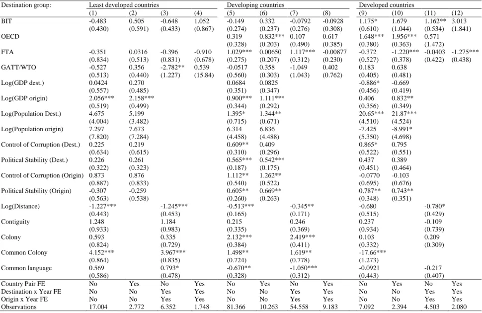
For least developed countries, GDP and population are not crucial determinants of investment flows. Instead, distance and sharing the same colonial ties play an important role. Surprisingly, estimation suggests that political variables such as control of corruption and political stability also do not play an important role in determining FDI on LDC. However, this is not true for developing countries. Estimation in columns (5-6) shows that both destination and origin political variables are statistically significant and have a strong economic impact. For developed countries, both political stability and control of corruption are statistically insignificant. Our results are consistent with the findings of Wei (2000) that control of corruption play a major role in the determination of FDI for developing countries. Our results suggest some degree of non-linearity of the effect of political risk on FDI since it depends heavily on the degree of development of the destination. Interestingly, political stability of the origin is positive and significant for both developing and developed countries but insignificant for LDC. We will return to this non-linearity of political risk on FDI in section 0.
Among the market size variables, the impact of GDP of the origin are positive and statistically significant on FDI for all groups, whereas population of the destination is significant for both developing and developed countries. Notably, the population has a tremendous impact on FDI for developed countries as it has an elasticity of 20 whereas the same elasticity is roughly one for developing (see columns 5-6 and 9-10).
More importantly and surprisingly, the estimates find statistically insignificant effects of BITs for least developed and developing countries. If there are any beneficiary from the BITs, the estimates suggest it might be the developed countries. Columns 9 and 11 show statistically significant effects at 10% and 5%, respectively. However, when controlling for multilateral resistance, these effects vanish as indicated by columns 10 and 12. Therefore, the estimates imply that BITs do not play an important role in the determination of FDI of least developed and developing countries and have at most mixed results for developed countries.
To further evaluating this claim, we also disaggregate the results by origin. i.e., for each destination group, we run the PPML estimation for two groups of origin countries: developing and developed. In this manner, our results can be directly compared with the ones in the literature. Even if the decision making of investors of different origin countries are similar as we argue, there is potentially one advantage of separating origin countries by their development level.
Table 2. The impact of BITs on foreign direct investments by destination group: PPML estimator
Destination group: Least developed countries Developing countries Developed countries
(1) (2) (3) (4) (5) (6) (7) (8) (9) (10) (11) (12) BIT -0.483 0.505 -0.648 1.052 -0.149 0.332 -0.0792 -0.0928 1.175* 1.679 1.162** 3.013 (0.430) (0.591) (0.433) (0.867) (0.274) (0.237) (0.276) (0.308) (0.610) (1.044) (0.534) (1.841) OECD 0.319 0.832*** 0.107 0.617 1.648*** 1.956*** 0.571 (0.328) (0.203) (0.490) (0.385) (0.380) (0.363) (1.472) FTA -0.351 0.0316 -0.396 -0.910 1.029*** 0.00650 1.117*** -0.00877 -0.372 -1.220*** -0.0403 -1.275*** (0.834) (0.513) (0.831) (0.678) (0.275) (0.207) (0.312) (0.230) (0.527) (0.378) (0.422) (0.438) GATT/WTO -0.527 0.356 -2.782** 0.539 -0.0517 0.358 -1.049 0.402 0.183 0.638 (0.513) (0.440) (1.227) (15.84) (0.560) (0.303) (1.043) (0.762) (0.405) (0.481) Log(GDP dest.) 0.0424 0.270 0.0684 0.0825 -0.886* -0.669 (0.557) (0.485) (0.351) (0.347) (0.456) (0.419) Log(GDP origin) 2.056*** 2.158*** 0.900*** 1.111*** 0.406 0.832** (0.519) (0.499) (0.344) (0.292) (0.356) (0.349) Log(Population Dest.) 4.675 5.199 1.395* 1.344** 20.65*** 21.87*** (4.004) (3.482) (0.715) (0.671) (4.510) (4.524) Log(Population origin) 7.297 7.673 6.314 6.836 -7.425 -8.991* (7.820) (7.284) (4.458) (4.488) (5.350) (4.698)
Control of Corruption (Dest.) 0.225 0.219 0.609** 0.409 0.865* 0.795
(0.634) (0.615) (0.310) (0.296) (0.522) (0.551)
Political Stability (Dest.) 0.226 0.261 0.565*** 0.542*** 0.437 0.389
(0.322) (0.323) (0.187) (0.175) (0.451) (0.464)
Control of Corruption (Origin) 0.873 0.876 1.112** 1.262** -0.0770 -0.103
(0.887) (0.833) (0.540) (0.522) (0.695) (0.676)
Political Stability (Origin) -0.307 -0.259 0.605** 0.669** 0.787** 0.743**
(0.563) (0.538) (0.260) (0.263) (0.348) (0.351) Log(Distance) -1.227*** -1.245*** -0.513*** -0.345** -0.680 -0.780* (0.443) (0.453) (0.165) (0.171) (0.515) (0.429) Contiguity 1.248 1.184 0.215 0.246 0.237 -0.109 (0.933) (0.983) (0.335) (0.369) (0.934) (0.739) Colony 0.593 0.335 2.132*** 2.419*** 0.103 0.209 (0.824) (0.729) (0.384) (0.411) (0.332) (0.309) Common Colony 4.152*** 3.967*** 1.498** 1.619** -17.66*** (0.864) (0.835) (0.724) (0.778) (1.273) Common language 0.569 0.793* -0.670** -1.050*** -0.0921 -0.217 (0.586) (0.478) (0.328) (0.312) (0.443) (0.407)
Country Pair FE No Yes No Yes No Yes No Yes No Yes No Yes
Destination x Year FE No No Yes Yes No No Yes Yes No No Yes Yes
Origin x Year FE No No Yes Yes No No Yes Yes No No Yes Yes
Observations 17.004 2.772 6.352 1.748 81.366 10.263 54.558 9.183 7.092 2.394 4.503 2.080
Note: * Significant at 10%; **Significant at 5%; ***Significant at 1%. Regressions include Origin, destination and year fixed effects. On the bottom of the table, additional specifications for fixed effects are available. Country-pair clustered standard errors in parenthesis.
Since our measure of BIT is a dummy variable, it does no distinguish the content of the BITs. Suppose that BITs among developing countries, and between developed and developing countries are very different regarding the contents, for instance. In that case, their capacity of generating additional foreign investment could differ. Under such circumstances, it would be beneficial to estimate the impact of those BITs separately.
Table 3 shows the results of such an exercise. For expositional convenience, we show results of the more complete specifications, with multilateral resistance only, and with country-pair fixed effects and multilateral resistance. Also, we restrict our attention to developing and developed countries as the origin of the FDI. Least developed countries as investors is a tiny fraction of total FDI, but more importantly, in most specifications, it is entirely explained by the country-pair fixed effects, which implies that LDC countries have very specifically destinations for their investments.
For the LDC as a destination, separating for origin groups does not change much the results. When developing countries are origin, the impact of BITs is insignificant in column (1) and cannot be estimated in the specification in column (2) in Table 3, since all covariates are perfectly collinear with the country-pair fixed effects. This implies that signing a BITs and FTAs between the least developed and developing countries are quite specific. For developed countries as origin, the estimation suggest that the impact is even harmful, unless if country-pair fixed effects are controlled (see columns 3-4).
Surprisingly, the BITs signed between developing and developed countries do not seem to be effective in boosting FDI in either direction. Actually, there is weak evidence towards the opposite. In the case of foreign investment from developed into developing countries, controlling for multilateral resistance shows an insignificant impact whereas controlling for fixed effects leads to a negative, but significantly only at 10% (columns 7-8). In the opposite direction, the effect is insignificant when controlling for multilateral resistance, whereas controlling for fixed effects leads to even more pronounced negative and significant at 5% (columns 9-10).
Table 3. The impact of BITs on foreign direct investments by destination and origin groups: PPML estimator
Destination group: Least developed countries Developing countries Developed countries
Origin group: Developing countries Developed countries Developing countries Developed countries Developing countries Developed countries
(1) (2) (3) (4) (5) (6) (7) (8) (9) (10) (11) (12) BIT -0.709 -1.064*** 0.396 1.283** -0.521 -0.0914 -0.602* 0.495 -5.512** (0.672) (0.408) (1.279) (0.541) (0.539) (0.328) (0.336) (0.558) (2.344) OECD 0.303 1.128 (1.048) (1.596) FTA 1.302 -0.722 1.176* 1.204 1.291*** -0.141 1.987 -0.755** -1.235*** (0.796) (0.869) (0.609) (0.996) (0.366) (0.241) (1.419) (0.335) (0.453) GATT/WTO -3.551*** -0.638 (0.864) (0.731) Log(Distance) -1.499*** -2.280*** -0.0127 -0.460** 1.591*** -2.082*** (0.570) (0.711) (0.318) (0.208) (0.399) (0.383) Contiguity 3.572*** -0.798 0.465 13.28*** -2.152*** (1.386) (1.075) (0.486) (2.151) (0.812) Colony 0.422 4.077*** 1.884*** -8.367*** -0.656 (0.752) (1.280) (0.453) (1.409) (0.474) Common Colony 1.551 (1.208) Common language 0.886* -1.902 -0.826** 4.176*** 0.508* (0.536) (1.358) (0.347) (0.813) (0.268)
Country Pair FE No Yes No Yes No Yes No Yes No Yes No Yes
Destination x Year FE Yes Yes Yes Yes Yes Yes Yes Yes Yes Yes Yes Yes
Origin x Year FE Yes Yes Yes Yes Yes Yes Yes Yes Yes Yes Yes Yes
Observations 1.529 364 3.017 1.143 21.821 3.236 19.206 5.149 2.099 786 1.270 1.092
Note: * Significant at 10%; **Significant at 5%; ***Significant at 1%. Country-pair clustered standard errors in parenthesis.
Therefore, the FDI from developing countries into developed countries cannot explain the positive impact found in Table 2, which suggests that it is likely that this comes from the FDI between developed countries. Unfortunately, note that columns 11 and 12 do not have an estimated impact of BIT. This happens because the BITs among developed countries were all implemented during the 1960s
and 1970s.4 This implies that during the sample all developed countries have BITs among each other, so there is no control group, i.e., developed countries without a BIT to compare. When considering the impact of BITs among developing countries, the positive and significant at 5% in the simpler specification. However, when controlling for country-pair fixed effects, sign changes and statistical significance vanishes.
2.3. How our results can be reconciled with the literature?
As discussed previously, our results contrast with the findings of the literature, even when we restrict the sample to developing countries as hosts and developed countries as investors. This section explores two reasons that can explain why our results differ from the ones found in the literature.
First, in the literature estimating the impact of BITs on FDI, it is common to use robust standard errors instead of clustered standard errors (see Hallward-Driemeie, 2003; Egger and Pfaffermayr, 2004; Neumayer and Spess, 2005; Desbordes and Vicard, 2009). We evaluate if using both types of standard errors leads to similar results and discuss which alternative is more appropriated. Second, we assess if controlling for country-pair fixed effects and multilateral resistance affects the results. Using clustered errors and multilateral resistance fixed effects are standard for the gravity model literature for trade flows literature (see Head and Mayer (2014) for an overall discussion of gravity models).
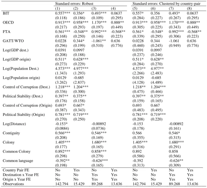
Table 4 shows the difference when using both for the PPML estimator. Of course, the parameters estimated in specifications (1-4) are the same as the ones in specifications (5-8). The only difference is the standard deviations, and thus, the statistical significance.
4 One exception is the BIT between Austria and Malta in 2004. These observations alone cannot generate enough variation for the estimation with country pair fixed effects and/or multilateral resistance fixed effects.
Table 4. Robustness to alternative standard errors
Standard errors: Robust Standard errors: Clustered by country-pair
(1) (2) (3) (4) (5) (6) (7) (8) BIT 0.557*** 0.356* 0.493*** 0.0637 0.557* 0.356 0.493* 0.0637 (0.118) (0.186) (0.109) (0.295) (0.284) (0.227) (0.267) (0.295) OECD 0.913*** 0.958*** 1.170*** 0.888** 0.913*** 0.958*** 1.170*** 0.888** (0.217) (0.293) (0.197) (0.449) (0.305) (0.225) (0.343) (0.449) FTA 0.561*** -0.548** 0.992*** -0.568** 0.561* -0.548* 0.992*** -0.568** (0.168) (0.250) (0.146) (0.223) (0.339) (0.295) (0.306) (0.223) GATT/WTO 0.0228 0.344* -1.061** 0.636 0.0228 0.344 -1.061 0.636 (0.296) (0.199) (0.510) (0.776) (0.460) (0.245) (0.949) (0.776) Log(GDP dest.) 0.0391 0.0997 0.0391 0.0997 (0.208) (0.188) (0.237) (0.246) Log(GDP origin) 0.511* 0.628*** 0.511* 0.628** (0.273) (0.229) (0.284) (0.270) Log(Population Dest.) 4.573*** 4.977*** 4.573** 4.977** (1.343) (1.293) (2.266) (2.483) Log(Population origin) 0.0129 -0.685 0.0129 -0.685 (3.262) (2.837) (4.128) (4.489)
Control of Corruption (Dest.) 1.218*** 1.204*** 1.218** 1.204***
(0.336) (0.300) (0.475) (0.466)
Political Stability (Dest.) 0.397** 0.375** 0.397** 0.375**
(0.176) (0.158) (0.159) (0.165)
Control of Corruption (Origin) 0.693* 0.667* 0.693 0.667
(0.387) (0.343) (0.483) (0.495)
Political Stability (Origin) 0.781*** 0.719*** 0.781*** 0.719***
(0.270) (0.250) (0.208) (0.220) Log(Distance) -0.153* -0.00892 -0.153 -0.00892 (0.0884) (0.0736) (0.178) (0.161) Contiguity 0.566*** 0.546*** 0.566 0.546* (0.208) (0.169) (0.355) (0.315) Colony 1.405*** 1.680*** 1.405*** 1.680*** (0.177) (0.165) (0.316) (0.291) Common Colony 0.892*** 0.858*** 0.892 0.858 (0.298) (0.279) (0.586) (0.566) Common language -0.392** -0.626*** -0.392 -0.626** (0.198) (0.165) (0.313) (0.309)
Country Pair FE No Yes No Yes No Yes No Yes
Destination x Year FE No No Yes Yes No No Yes Yes
Origin x Year FE No No Yes Yes No No Yes Yes
Observations 142.794 15.429 89.268 13.636 142.794 15.429 89.268 13.636
Note: * Significant at 10%; **Significant at 5%; ***Significant at 1%. Regressions include Origin, destination and year fixed effects. On the bottom of the table, additional specifications for fixed effects are available.
Particularly for the coefficient measuring the impact BITs, using robust standard errors leads to smaller standard errors, and therefore, greater the statistical significance.
So, which standard deviation should be used? As discussed by Cameron and Miller (2005), there is no objective criterion for choosing whether or how to cluster the standard errors, but there are two recommendations. First, whenever it is known that there is a correlation of the covariates in a particular dimension. In the case the gravity equation for FDI, this happens naturally. For instance, gravity variables such as distance, colonial history, contiguity, and language do not vary over time. Therefore, within the country-pair, those variables are perfectly correlated.
Moreover, for controls such as GDP, Population, and political variables, which vary over time but are constant within the partner (they are constant for the origin when the variables are for the destination and vice-versa). Again, there is a perfect correlation in these dimensions. Therefore, since the country-pair clusters incorporate both destination and origin clusters, country-pair standard errors are the safest choice of cluster given the data structure. The second reason is related to the correlation of the errors. In this case, the country-pair clusters can account for autocorrelation within each country-country-pair error, which is assumed zero in the robust case. This is likely to happen since we are using a relative long time dimension in the panel.
Even if robust standard errors are considered an appropriate choice, note that as long as one control for multilateral resistance and country-pair fixed effects, the impact of BITs on FDI becomes statistically insignificant (compare columns 2 and 4). Our results suggest that the positive impact found in the literature is owing to a combination of using robust standard errors without controlling for multilateral resistances. If either of them is used, the statistical significance of the BIT vanishes.
2.4. The role of Political risk on BIT impacts on FDI
One of the main arguments for BITs to boost FDI is owing to decreasing uncertainty, improving the regulatory security and mitigating expropriation risks. Moreover, BITs not only comply countries to commit not to expropriate investors but also ensure the possibility of firms repatriating profits without much delay.
If BITs induce this better investment environment, it would be natural that to lead to higher foreign investment, all else constant. Under this argument, countries with less developed institutions could use BITs as an alternative to build credibility and increase their attractiveness to foreign investment. In that sense, BITs can be seen as substitutes for improvements in institutional quality, which can be much more difficult to implement. On the other hand, if the capability of inducing credibility through the BITs depend if the country has at least some level of institutional quality, BITs can be seen as complements of institutional quality.
Following Hallward-Driemeie (2003), which was the first to evaluate if the impact of BITs depends on the institutional quality, we augment equation (1) by introducing interactions term of BIT with both political stability and control of corruption of the destination country such that
𝐹𝑖𝑗𝑡 = exp(β𝐵𝐼𝑇𝑖𝑗𝑡+ 𝛾𝑐𝑐𝐵𝐼𝑇𝑖𝑗𝑡× 𝐶𝐶𝑗𝑡+ 𝛾𝑝𝑠𝐵𝐼𝑇𝑖𝑗𝑡× 𝑃𝑆𝑗𝑡+ 𝑿𝑖𝑗𝑡𝜃 + 𝛼𝑖 + 𝛾𝑗+ 𝜂𝑡) + 𝜀𝑖𝑗𝑠𝑡, (2) where 𝐶𝐶𝑗𝑡 and 𝑃𝑆𝑗𝑡 denote control of corruption and political stability of the destination country, respectively.5
5 As before the vector of controls, 𝑿
Table 5 shows the results for the specification (2), which we also test if the effects are heterogeneous depending on destination country development group as in the previous section. The iteration of BIT with political stability is strongly negative and statistically significant for all specifications for the least developed countries while it is insignificant for the other country groups (except the specification 10 for developed countries, but only at 10% significance). On the other hand, the interaction of BIT with the control of corruption is also strongly negative and significant in almost all specifications of developing and developed countries (except the specification 6, for developing countries). It is noteworthy that when controlling for both fixed effects and multilateral resistance, the coefficients are significant at only at 10% significance (columns 8 and 12). In the case of developed countries, the negative coefficient of the interaction is opposed by the quite high positive coefficient for BIT with the same significance pattern. This is not the case for developing countries.
After all, what does it mean to have a negative interaction? Recall that our political variables are standardized, i.e., mean zero and unit variance. For instance, the negative coefficient of the interaction of BIT and political stability in column (1-4) implies that a country with one standard deviation higher (lower) than the mean value has a negative (positive). In other words, countries with relatively poor institutional quality enjoy higher benefits of BITs whereas countries with relatively strong political stability have lower benefits (or might even loss some of the foreign investment) of BITs. Therefore, our estimations suggest that the interpretation of BITs as substitute to intuitional quality.
More interestingly, the type of institutional quality matters, depending on the destination group. The estimation suggests that for LDC, which are much less stable countries in terms of investment environment, BITs can be used as substitutes to the lack of political stability. The fact that the interaction with control of corruption is insignificant within the LDC suggests that control of corruption, for countries that severely suffer from political stability, this may be a lesser issue. When countries transit to developing countries, there is an improvement in terms of institutional quality, political stability does not seem to be a concern, but the control of corruption becomes a more pressing issue. The same is true for developed countries with even higher institutional quality. Note that the average values for least developing, developing and developed countries for political stability are -0.60, 0.01 and 1.04 (all statistically different from each
other), respectively. This narrative is consistent with the significance shifting from political stability to control of corruption observed in Table 5 by comparing the results from columns (1-4) with the ones in columns (5-6) and (9-12).
Our results contrast with the results found by Hallward-Driemeie (2003) that found complementarities between BIT and institutional quality. Desbordes and Vicard (2009) also highlight that there are complementarities between BITs with institutional quality and interstate relations. Both studies focus only in the FDI flows from developed to developing countries. As Hallward-Driemeie (2003) points out “(…) it may be that a certain level of institutional capacity is needed before the BIT is seen as credible”. We argue that despite the substitutability of BITs and institutional quality that we found within each group, there is a margin for this interpretation when we compare between destination groups. As long as there a certain level of intuitional quality, political stability does not play a major role in the impact of BITs since the coefficients become insignificant. However, other types of institutional quality, such as control of corruption start to become more important.
Since the BIT is a dummy variable, the overall impact of BITs on the FDI in can be computed by exp(𝛽 + 𝛾𝑐𝑐𝐶𝐶𝑗𝑡+ 𝛾𝑝𝑠𝑃𝑆𝑗𝑡) − 1. By taking the average values of political stability for LDC (-0.60) and control of corruption for developing and developed countries (-0.07 and 1.66, respectively), we can compute the overall effect at the mean. Using the more specification with fixed effects and multilateral resistance (columns 4, 8 and 12) and considering only the coefficients statistically significant at 10% or less, the estimated marginal effects at the mean are 1.73, 0.05 and 3.90, respectively. In other words, BITs for LDC and developed countries increase the FDI roughly by 2.7 and 5 times, respectively. The estimation suggests that developing countries are much less benefited from the BITs, increasing their FDI only bit 5%.
Table 5. Bilateral investment treaties and institutional quality
Destination group: Least developed countries Developing countries Developed countries
(1) (2) (3) (4) (5) (6) (7) (8) (9) (10) (11) (12)
BIT -1.633* -0.169 -2.443** -0.805 -0.0712 0.190 0.0113 -0.295 3.864*** 4.985** 3.527*** 5.845*
(0.957) (0.924) (1.058) (1.273) (0.272) (0.306) (0.274) (0.309) (0.784) (2.127) (0.756) (3.518) BIT*Control of Corruption (Dest.) -0.368 -1.042 -0.652 -1.166 -0.712*** -0.611 -0.805*** -0.697* -1.562*** -2.974*** -1.268*** -2.560* (0.871) (1.147) (0.907) (0.988) (0.251) (0.460) (0.256) (0.371) (0.382) (0.980) (0.408) (1.539) BIT*Political Stability (Dest.) -1.010** -0.618 -1.411*** -1.668*** 0.218 -0.271 0.330 -0.590 -0.121 1.620* -0.332 1.215
(0.402) (0.473) (0.422) (0.576) (0.213) (0.309) (0.254) (0.367) (0.767) (0.866) (0.992) (1.238) OECD 0.338 0.823*** 0.157 0.623 1.683*** 1.947*** 0.808 (0.329) (0.203) (0.511) (0.391) (0.377) (0.367) (1.488) FTA -0.0315 -0.0982 0.164 -0.780 0.993*** 0.0237 1.060*** 0.0159 -0.366 -1.217*** -0.0320 -1.277*** (0.826) (0.599) (0.869) (0.679) (0.280) (0.209) (0.317) (0.233) (0.528) (0.379) (0.418) (0.438) GATT/WTO -0.307 0.320 -2.401** 1.339 0.00370 0.355 -0.940 0.393 0.388 0.504 (0.522) (0.467) (0.556) (0.302) (1.031) (0.776) (0.455) (0.420) Log(GDP dest.) -0.127 0.181 0.0539 0.0772 -0.893** -0.686 (0.522) (0.467) (0.350) (0.342) (0.455) (0.420) Log(GDP origin) 2.010*** 2.147*** 0.869** 1.099*** 0.425 0.760** (0.533) (0.538) (0.345) (0.295) (0.348) (0.371) Log(Population Dest.) 5.157 5.051 1.407** 1.272* 20.73*** 21.92*** (4.109) (3.898) (0.706) (0.684) (4.505) (4.495) Log(Population origin) 7.426 7.647 6.257 7.008 -7.530 -8.372* (7.748) (6.926) (4.451) (4.478) (5.321) (4.902)
Control of Corruption (Dest.) 0.448 0.563 0.819** 0.655* 0.891* 0.834
(0.723) (0.652) (0.325) (0.381) (0.524) (0.562)
Political Stability (Dest.) 0.480 0.415 0.511** 0.593*** 0.444 0.383
(0.362) (0.374) (0.200) (0.204) (0.450) (0.469)
Control of Corruption (Origin) 0.934 0.761 1.141** 1.289** -0.0901 -0.0485
(0.917) (0.828) (0.541) (0.528) (0.693) (0.696)
Political Stability (Origin) -0.273 -0.287 0.609** 0.702*** 0.776** 0.738**
(0.546) (0.528) (0.257) (0.265) (0.351) (0.350) Log(Distance) -1.061** -1.038** -0.541*** -0.374** -0.689 -0.787* (0.423) (0.437) (0.160) (0.165) (0.510) (0.425) Contiguity 1.448 1.336 0.189 0.192 0.230 -0.115 (0.969) (1.032) (0.336) (0.372) (0.932) (0.734) Colony 0.665 0.412 2.217*** 2.496*** 0.159 0.262 (0.819) (0.670) (0.371) (0.397) (0.343) (0.315) Common Colony 4.260*** 3.903*** 1.370** 1.495** -17.68*** (0.830) (0.821) (0.685) (0.746) (1.267) Common language 0.600 0.916** -0.844** -1.211*** -0.0980 -0.220 (0.553) (0.447) (0.337) (0.317) (0.444) (0.408)
Country Pair FE No Yes No Yes No Yes No Yes No Yes No Yes
Destination x Year FE No No Yes Yes No No Yes Yes No No Yes Yes
Origin x Year FE No No Yes Yes No No Yes Yes No No Yes Yes
Observations 17.004 2.772 6.352 1.748 81.366 10.263 54.558 9.183 7.092 2.394 4.503 2.080
Note: * Significant at 10%; **Significant at 5%; ***Significant at 1%. Regressions include Origin, destination and year fixed effects. On the bottom of the table, additional specifications for fixed effects are available.
3.
Final Remarks
This report provides a comprehensive study of the impact of bilateral investment treaties for a sample of 197 countries in the period 2001-2012. By comprehensive, we mean that we are considering all possible directions of foreign investment regardless of their level of development. We also revisit some of the existing results of the literature estimating the impact of BIT on FDI for a specific investment direction: from developed countries into developing countries.
We find evidence weak evidence of an unconditional impact of a BIT on foreign investment. Results for least developed and developing countries are insignificant for all specifications. For developed countries, there is some evidence and positive and statistically significant impact of BITs for specifications without fixed effects. When controlling for fixed effects – which we argue that is essential since it better controls for the decision of signing the BITs – the estimated impacts become statistically insignificant.
However, we find evidence that the impact of BITs on FDI depending on the institutional quality. Specifically, we find that BITs have a stronger impact in countries with poor institutional quality, i.e., our results suggest that BITs are substitutes to improvements the institutional quality that diminish the perceived risk of foreign investment. More interestingly, the most important indicator for the least developed countries is political stability, whereas control of corruption plays a major role in the impact of BITs for developing and developed countries. This suggests that investors’ concerns regarding least developed countries are more pronounced than for developing and developed countries, but BITs can mitigate such concerns for all destinations’ development levels.
Finally, our results imply that the direction of the flow matters. Considering the average institutional quality, the estimated impact of BITs at the mean is to increase the FDI in, 270%, 5%, and 390%, for least developed, developing and developed countries, respectively. Therefore, developed and least developed countries are the most benefited from bilateral investment treaties whereas developing countries marginally increase their FDI with such agreements, on average.
References
Anderson, J.E., van Wincoop, E., 2003. Gravity with gravitas: a solution to the border puzzle. American Economic Review 93 (1), 70– 192.
Baier, S.L., Bergstrand, J.H., 2007. Do free trade agreements actually increase members’ international trade? Journal of International Economics 71 (1), 72–95.
Bergstrand, J.H., Egger, P., 2008. A knowledge-and-physical-capital model of international trade flows, foreign direct investment, and multinational enterprises. Journal of International Economics 73 (2), 278–308.
Cameron A.C., Miller D.. 2015. A Practitioner’s Guide to Cluster-Robust Inference. Journal of Human Resources 50(2):317–72 Carr, D., Markusen, J. R. and Maskus, K. E.: 2001, Estimating the knowledge-capital model of the multinational enterprise, American Economic Review 91, 693–708.
Desbordes, R., Vicard, V 2009. Foreign direct investment and bilateral investment treaties: an international political perspective. Journal of Comparative Economics, vol 37, no. 3, pp. 372-386
Hallward-Driemeier, M., 2003. Do bilateral investment treaties attract foreign direct investment? only a bit. . . and they could bite, World Bank Working Paper, No. 3121.
Head, K., Mayer, T., 2014. ‘‘Gravity Equations: Workhorse, Toolkit, Cookbook,’’ Handbook of International Economics, vol. 4, Gita Gopinath, Elhanan Helpman, and Kenneth Rogoff, eds, pp. 131-195.
Head, K., Ries, J., 2008. FDI as an outcome of the market for corporate control: theory and evidence. Journal of International Economics 74 (1), 2–20.
Feenstra, R.C., 2004. Advanced International Trade: Theory and Evidence. Princeton University Press, Princeton.
Neumayer, E., Spess, L., 2005. Do bilateral investment treaties increase foreign direct investment to developing countries? World Economy 33 (10), 1567–1585.
Santos Silva, J., Tenreyro, S., 2006. The log of gravity. Review of Economics and Statistics 88 (4), 641–658.
UNCTAD, 2006. Bilateral Investment Treaties 1995-2006: Trends in Investment Rulemaking.