Results from the Dixit/Stiglitz
monopolistic competition model
Richard Foltyn
February 4, 2012
Contents
1 Introduction 1
2 Constant elasticity sub-utility function 1
2.1 Preferences and demand . . . 1
2.1.1 General case . . . 2
2.1.2 Cobb-Douglas case (“Dixit-Stiglitz lite”) . . . 7
2.2 Firms and production . . . 8
2.3 Market equilibrium . . . 8
1 Introduction
The Dixit/Stiglitz monopolistic competition model has been widely adopted in various fields of economic research such as international trade. The Dixit and Stiglitz (1977) paper actually contains three distinct models, yet economic literature has mostly taken up only the first one (constant elasticity case) and its market equilibrium solution. The main results of this subset of Dixit and Stiglitz (1977) are derived and explained below in order to aid in understanding this widespread model.
2 Constant elasticity sub-utility function
2.1 Preferences and demand
Assumption 2.1. Preferences are given by a (weakly-)separable, convex utility function
u=U(x0, V(x1, x2, . . . , xn))
whereU(·) is either a social indifference curve or the multiple of a representative consumer’s
utility. x0is a numeraire good produced in one sector whilex1, x2, . . . , xn are differentiated
goods produced in another sector.1
1
Dixit and Stiglitz (1977) treat three different cases in which they alternately impose two of the three following restrictions:
1. symmetry ofV(·) w.r.t. to its arguments;
2. CES specification forV(·)
3. Cobb-Douglas form forU(·)
However, throughout the literature many authors have imposed all three restrictions together in what Neary (2004) calls “Dixit-Stiglitz lite”.
The next section examines the more general case in which only restrictions 1 and 2 are imposed. Subsection 2.1.2 briefly looks and the more special case of “Dixit-Stiglitz lite”.
2.1.1 General case
First-stage optimization.
Assumption 2.2. In the CES case the utility function is given as
u=U
x0,
" X
i
xρi
#1/ρ
with ρ ∈ (0,1) to allow for zero quantities and ensure concavity of U(·). ρ is called the
substitution or “love-of-variety” parameter.2 Furthermore,U(·) is assumed to behomothetic
in its arguments.
SinceU(·) is a separable utility function, the consumer optimization problem can be solved
in two separate steps: first the optimal allocation of income for each subgroup is determined, then the quantities within each subgroup.
Definition 2.1. Let y be a quantity index presenting all goods x1, x2, . . . , xn from the
second sector such that
y≡
" X
i
xρi
#1/ρ
. (1)
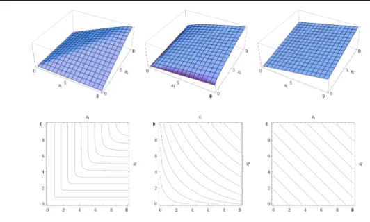
Figure 1 shows some illustrative examples for the two-dimensional case. As required, the utility function is concave and x1, x2 are neither complements nor perfect substitutes if
ρ∈(0,1).
The first-stage optimization problem is given as follows:
max. U(x0, y)
s.t. x0+q·y=I
whereI is the income in terms of the numeraire andqis the price index ofy.3
2
WithP ρ= 1,x1, . . . , xnare perfect substitutes as the subutility function simplifies toV(x1, x2, . . . , xn) =
ixiand thus it does not matter whichxiis consumed. Forρ <0 they are complements (see Brakman
et al. 2001, 68).
3
Figure 1:CES functions with two-dimensional domain and varyingρparameter (from left to right: ρ= {-10, 0.5, 0.99}). The first case is excluded in this model due to the restrictions on parameterρ.
From the LagrangianL=U(x0, y)−λ[x0−qy−I] we obtain the first-order conditions
∂L
∂x0
=U0−λ= 0 (2)
∂L
∂y =Uy−λq= 0 (3)
∂L
∂λ =x0+qy−I= 0 From (2) and (3) we get the necessary condition
Uy
U0
=q=py p0
(4)
which is the familiar Ui/Uj = pi/pj as q is the price index for y and p0 = 1 due to the
numeraire definition. SinceU(·) was assumed homothetic, this uniquely identifies the share
of expenditure forx0andybecause these solely depend on relative marginal utilities. Denote
the share of expenditure onyass(q) and that onx0as (1−s(q)). Then the optimal quantities
for each sector are
x0= (1−s(q))I
y=s(q)I
q (5)
Second-stage optimization. Given the definition ofy ands(q), the second-state problem is
max. y=
" X
i
xρi
#1/ρ
s.t. X
i
The LagrangianL= (P ix ρ i) 1/ρ− λ(P
ipixi−s(q)I) yields the first-order conditions
∂L
∂xi
=y1−ρxρ−1
i −λpi= 0 (6)
∂L
∂λ =
X
i
pixi−s(q)I= 0 (7)
Solving (6) forxi gives
xi=y(λpi)1/(ρ−1) (8)
Inserting this into (7) and solving forλwe get
X
i
piy(λpi)1/(ρ−1)=s(q)I
λ1/(ρ−1)yX
i
pρ/(ρ−1)
i =s(q)I
λ1/(ρ−1)=s(q)I) y
" X
i
pρ/(ρ−1)
i
#−1
(9)
Finally, plugging (9) back into (8) we get the preliminary demand function facing a single firm in the second sector:4
xi=s(q)Ip1/(ρi −1)
X
j
pρ/(ρ−1)
j
−1
(10)
To further simplify this expression, take (10) to the power ofρand sum overi:5
xρi = (s(q)I)ρpρ/(ρ−1)
i
X
j
pρ/(ρ−1)
j −ρ X i
xρi =
X
j
pρ/(ρ−1)
j
−ρ
(s(q)I)ρX
i
pρ/(ρ−1)
i
y=
" X
i
xρi
#1/ρ = X j
pρ/(ρ−1)
j −1 s(q)I " X i
pρ/(ρ−1)
i
#1/ρ
y= s(q)I
h P
ip ρ/(ρ−1)
i
i(ρ−1)/ρ (11)
From (5) and (11) we obtain
Result 2.1. For the utility function given in Assumption 2.2 and the composite quantity index from Definition 2.1 the correspondingprice index is
q=
" X
i
pρ/(ρ−1)
i
#(ρ−1)/ρ
(12)
4
The summation index has been changed tojto reflect that it in is unrelated toi.
5
Using Result 2.1, (10) can be simplified to arrive at
Result 2.2. For the utility function given in Assumption 2.2, the resultingdemand function facing a single firm is
xi=y
q pi
1/(1−ρ)
(13)
withy andqdefined in (1) and (12), respectively.
Some remarks regarding the demand function and CES preferences are in order.
First, by plugging y = s(q)I/q into (13) and taking logs, it can easily be seen that the varietiesx1, x2, . . . , xn have unitincome elasticities ∂logxi/∂logI.
Second, assuming a sufficiently large number of varieties so that pricing decisions of a single firm do not affect the general price index, theprice elasticity of demand forxi is
ǫd=
∂logxi
∂logpi
q const.
= 1
ρ−1 (14)
At this point it is convenient to defineσ≡1/(1−ρ) so thatǫd=−σ.6
Third, to get theelasticity of substitution between two varieties, from (6) we see that
xi
xj
=
pj
pi
1/(1−ρ)
and hence the elasticity of substitution can be obtained as
ǫs=∂log(xj/xi)
∂log(pi/pj)
= ∂log(pi/pj)
1/(1−ρ) ∂log(pi/pj)
= 1
1−ρ =σ (15)
This can be summarized as
Result 2.3. Dixit-Stiglitz preferences given in Assumption 2.2 result inconstant demand and substitution elasticities given by
ǫd=
1
ρ−1 =−σ ǫs=
1 1−ρ =σ
Often the model is specified directly in terms ofσinstead ofρ,7 with
u=U(x0, y), y≡
" X
i
x1−1/σ
i
#1/(1−1/σ)
, q≡
" X
i
p1−σ
i
#1/(1−σ)
Fourth, to see why the CES utility specification is called “variety-loving”, inspect the large-subgroup case with many varietiesnwith similar price levels, i.e. pi≈pand hencexi=x.
Then expenditure is equally divided over all varietiesx1, x2, . . . , xnsince they symmetrically
6
Hereσis different fromσ(q) in Dixit and Stiglitz (1977), but reflects the notation of many other Dixit-Stiglitz-based models.
7
enter into the subutility function. If there exist n varieties, the expressions for y and q simplify to
y=
" n X
i
xρ
#1/ρ
=xn1/ρ (16)
q=
" n
X
i
pρ/(ρ−1)
#(ρ−1)/ρ
=pn(ρ−1)/ρ (17)
Plugging (5) and (17) into (13) gives a simplified demand function for the large-subgroup case:
x=s(q)I
np . (18)
Substituting this forxin the subutility function (1), we obtain
V(n) =y=
" n X
i
s(q)I
np
ρ#1/ρ
=n(1/ρ)s(q)I np =n1/ρ−1(nx)
which is increasing innasρ∈(0,1) by assumption. The last equality provides some intuitive
insights: since (nx) is the actual quantity produced, the term n1/ρ−1 >1 can be seen as an additional “bonus”, so variety represents an externality or the extent of the market. Increasing the market sizenxhas a more than proportional effect on utility due to this term (Brakman et al. 2001, 68).
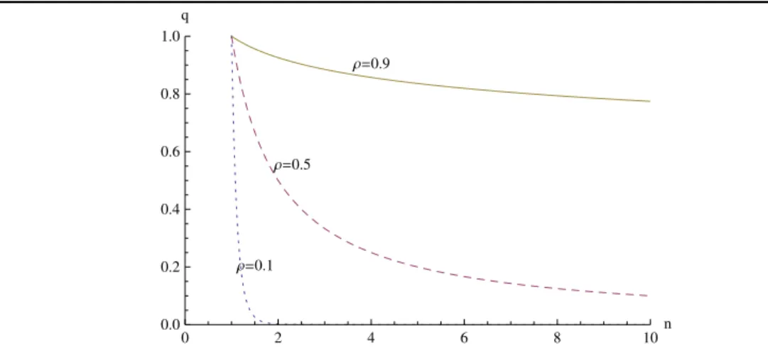
That utility increases with variety can also be seen by recalling thatV(x) =y =s(q)I/q and examining howqfrom (17) changes withn, as shown in Figure 2.
Figure 2:Price indexqas a function of the number of varietiesn(assumingp= 1)
Ρ=0.1 Ρ=0.5
Ρ=0.9
0 2 4 6 8 10n
0.0 0.2 0.4 0.6 0.8 1.0 q
2.1.2 Cobb-Douglas case (“Dixit-Stiglitz lite”)
In this section we inspect a special case of the model in which all three of the initially mentioned restrictions on utility are imposed.
Assumption 2.3. IfU(·) is Cobb-Douglas and V(·) is CES, the resulting utility function
is given by
u=U(x0, y) =x10−αyα.
Again a two-state optimization approach is applicable.
First-stage optimization. The maximization problem is stated as follows:
max. u=x1−α
0 yα (19)
s.t. x0+qy=I
As in (4), the necessary condition from the Lagrangian is Uy/U0=q, which together with
the budget constraint yields the well-known result for Cobb-Douglas utility:
x0= (1−α)I (20)
y=αI
q (21)
Second-stage optimization. From here the second-stage optimization proceeds exactly as in the general case, withαreplacings(q). Using the definition ofqone arrives at the demand function given in Result 2.2.
With the Cobb-Douglas / CES case it can easily be verified that a single-stage optimization process yields the same results. The Lagrangian in this case is
L=x1−α
0
" X
i
xρi
#α/ρ
−λ
"
x0+
X
i
pixi−I
#
with the relevant first-order condition being
∂L
∂xi
=x(1−α)
0
α ρ
" X
i
xρi
#(α−ρ)/ρ ρxρ−1
i −λpi= 0
demand function can be obtained:
xi
xj
=
pi
pj
1/(ρ−1)
pixi=pρ/(ρi −1)p 1/(1−ρ)
j xj
I−x0=X
i
xipi=p1/(1j −ρ)xj
X
i
pρ/(ρ−1)
i
xj =
(I−x0)p1/(ρ−1)
j
P
ip ρ/(ρ−1)
i
=I−x0 q
q1/(1−ρ) p1/(1−ρ)
j
[by def. ofq]
=y
q
pj
1/(1−ρ)
2.2 Firms and production
It is assumed that all firms producing varieties of xi have identical fixed and marginal
costs. Since consumers demand all existing varieties symmetrically, any new firm entering the market will choose to produce a unique variety and exploit monopolistic pricing power instead of entering into a duopoly with an existing producer. Also, every firm will choose to produce one variety only (see Baldwin et al. (2005, 42) on how to derive this result).
Production for each firm exhibits (internal) increasing returns to scale. This is implied by introducing fixed costs in addition to (constant) marginal costs as stated above. Hence the cost function has the form
C(x) =cx+F (22)
where c is the marginal costs and F the fixed cost per variety (there are no economies of scope).8
2.3 Market equilibrium
Equilibrium in this model is determined by two conditions: first, firms maximize profits consistent with the demand function (13); second, as this creates pure profit which induces new firms to enter the market, quantities ofxi adjust until the marginal firm just breaks
even (free entry condition).
Profit maximization. Since each firm produces a unique variety, monopolistic pricing ap-plies and each firm faces the maximization problem
max. π=p(x)x−cx−F (23)
It is assumed that each firm takes price setting behavior of other firms as given (other firms do not adapt their prices as a reaction to the firm’s price) and that firms ignore effects of their pricing decisions on the price indexq. Again, this assumption is only plausible with a sufficiently large number of firms.
8
The necessary first-order condition resulting from (23) is the well-known
p
1 + 1 ǫd
=c
p
1−1
σ
=c
whereǫdis the elasticity of demand, which was shown to equal−σ= 1/(ρ−1) in Result 2.3.
Solving forp, we obtain
Result 2.4. In equilibrium, the optimal price is given by
pe=
c ρ ,
wherepeis calculated as aconstant mark-up over marginal costc.
Free entry condition. As the model assumes free entry, new firms will enter the market and produce a new variety as long as this yields positive profit. When a firm enters the market and starts producing a new variety, consumers divert some of the expenditure previously spent on existing varieties to purchase the new good. The quantity of each variety sold decreases, as does profit due to rising average costs. As a consequence, the free entry condition states that in equilibrium the marginal firm (indexed byn) just breaks even, i.e. operating profit equals fixed cost:9
(pn−c)xn=F (24)
With symmetry and identical firms, condition (24) holds for all intramarginal firms as well. Solving (24) forx, we get
Result 2.5. The free entry condition dictates that in equilibrium the quantity of each variety produced is
xe= F
pe−c =
F
c(σ−1). (25)
Naturally, in equilibrium the number of varieties produced has to be consistent with the demand function from (18), and therefore
s(pen(ρe−1)/ρ)
pene
= F
(pe−c)
(26)
must hold. This uniquely identifies an equilibrium if the left-hand side is a monotonic function ofn, which is the case if the elasticity w.r.t.nhas a determinate sign. It is assumed to be negative as the quantity of each variety consumed decreases when more varieties are available. See Dixit and Stiglitz (1977, 300) for a formal condition for this to hold.
Before finishing this section, some further remarks regarding the equilibrium are necessary. First, from (25) it can be seen that equilibrium quantities are constant and depend on the two cost parameters,F andc, and on one demand parameter,σ, all of which are exogenously determined. They are independent of other factors such as the number of varieties produced. Therefore, aggregate manufacturing output can only increase by increasing the number of
9
varieties. This determines the outcome of models such as Krugman (1980), where increasing the market size via trade liberalization results in more varieties, not higher quantities per firm.10
Second, calculating equilibrium operating profit (ignoring fixed costs) as
πe= (pe−peρ)xe
πe= (1−ρ)pexe
πe=pexe
σ
we see that operating profits are determined as a constant profit margin 1/σ of revenue pexe.
10
References
Baldwin, R. E., R. Forslid, P. Martin, G. I. P. Ottaviano, and F. Robert-Nicoud (2005). Economic geography and public policy. Princeton, N.J.: Princeton Univ. Press.
Brakman, S., H. Garretsen, and C. van Marrewijk (2001). An introduction to geographical economics. Cambridge: Cambridge Univ. Press.
Dixit, A. K. and J. E. Stiglitz (1977). Monopolistic competition and optimum product diversity. American Economic Review 67(3), 297–308.
Gravelle, H. and R. Rees (2004). Microeconomics (3rd ed.). Harlow: Pearson.
Krugman, P. R. (1980). Scale economies, product differentiation, and the pattern of trade. American Economic Review 70(5), 950–959.